IEEE SIGNAL PROCESSING LETTERS, VOL. 18, NO. 1, JANUARY 2011
11
Computationally Efficient Approaches to Aeroacoustic Source Power Estimation Lin Du, Petre Stoica, Jian Li, and Louis N. Cattafesta, III
Abstract—Two computationally efficient approaches are proposed for aeroacoustic source power estimation, under the assumption of a single dominant source contaminated by uncorrelated noise. The proposed methods are evaluated using both simulated and measured data. The numerical examples show that the proposed algorithms yield good power estimates even under low signal-to-noise ratio (SNR) conditions, and the experimental results show that the power estimates obtained via the proposed approaches are consistent with each other. Furthermore, the approaches are computationally much more efficient than the existing nonlinear least-squares (NLS) algorithm. Index Terms—Aeroacoustic source power estimation, covariance-based approaches.
I. INTRODUCTION EROACOUSTIC source power estimation is required in many wind-tunnel applications and has attracted much research interest for the past decades. Numerous methodologies involving acoustic array measurements have been proposed to address this issue [1]–[3]. The main challenge for the problem is to properly separate the aeroacoustic power information of the source of interest (SOI) from the extraneous noise, such as electronic noise and other flow-induced microphone self-noise sources, which are inevitable in any test facility. When a single dominant aeroacoustic SOI is concerned (e.g., trailing edge noise), some coherent-source based analysis techniques, such as coherent output power (COP) method and the three-microphone method can be used to isolate the SOI from the extraneous noise [3]. Both methods are simple but they require an appropriate selection of reference microphones, which is usually unclear in practice. To avoid this limitation, a nonlinear least-squares (NLS) algorithm has been presented with the intent of finding the “best fit” directivity. However, as discussed in [4], low signal-to-noise ratio (SNR) conditions at one or more microphones may degrade the NLS performance significantly. In order to achieve more reliable SOI power estimation, several iterative covariance-based approaches have been
A
Manuscript received September 08, 2010; revised October 11, 2010; accepted October 13, 2010. Date of publication October 21, 2010; date of current version November 18, 2010. This work was supported in part by NASA Cooperative Agreement NNX07AO15A, the Swedish Research Council (VR) and the European Research Council (ERC). The associate editor coordinating the review of this manuscript and approving it for publication was Dr. Mads Graesboll Christensen. L. Du and J. Li are with Department of Electrical and Computer Engineering, University of Florida, Gainesville, FL 32611-6130 USA (e-mail:
[email protected]. edu) P. Stoica is with Department of Information Technology, Uppsala University, SE-75105 Uppsala, Sweden. L. N. Cattafesta, III is with Department of Mechanical and Aerospace Engineering, University of Florida, Gainesville, FL 32611-6250 USA. Color versions of one or more of the figures in this paper are available online at http://ieeexplore.ieee.org. Digital Object Identifier 10.1109/LSP.2010.2089049
presented recently [5], which have been shown to provide much more accurate SOI power estimates than NLS. In this letter, we present several alternative approaches to SOI power estimation based on the spectral density covariance matrix of the microphone signals. Unlike the approaches in [5], the proposed methods have closed-form solutions, and therefore they are quite simple and do not need initial values or iterations. As demonstrated herein, the proposed techniques can remove the extraneous noise efficiently even under low SNR conditions. Notation denotes that each element of a vector is nonnegative. represents a diagonal matrix with its diagonal formed represents a column vector by the elements of , and formed by the diagonal elements of a matrix . and denote the real and imaginary parts of a complex-valued number, respectively. denotes the Euclidean norm for a vector or the Frobenius norm for a matrix. The superscripts , and denote the conjugate transpose, complex conjugate and transpose, respectively. II. DATA MODEL Consider a single-input multiple-output system, which represents an -microphone measurement of an acoustic field input generated by a single source but corrupted by extraneous noise. A realistic example is the measurement of trailing-edge noise considered in [1] and [4]. The observed measurement can be modeled as follows: (1) denotes the where denotes the convolution operator, and denote the channel impulse response SOI, and the extraneous noise contamination for the th channel, respectively. In the preprocessing stage, the time-domain observed data of each channel , , is divided into blocks and each block of data is then converted into narrowband frequency bins via the Fourier transform. From (1), the th channel output for a particular frequency bin can be modeled as (2) , and are the Fourier transwhere , and for the th block, respectively, forms of is the Fourier transform of . We will estimate and the SOI power levels independently for each frequency bin. For notational simplicity, the dependence on will be omitted. By stacking the data from all channels ( ) together, the model in (2) can be written in a compact vector form (3) where response,
1070-9908/$26.00 © 2010 IEEE
is the unknown channel frequency is the SOI, is the
12
IEEE SIGNAL PROCESSING LETTERS, VOL. 18, NO. 1, JANUARY 2011
observed data vector, and is the unknown noise vector and . is defined similarly to We assume that the extraneous noise is spatially uncorrelated between measurement channels and uncorrelated with the source signal . This assumption is reasonable as long as the extraneous noise is limited to device electronic noise and pressure fluctuations over the microphones generated by small-scale turbulence [4]. Under this assumption, we obtain the as follows: covariance matrix of
where
is an arbitrary orthogonal matrix, i.e., . Then we have
(11) Let , . Considering the diagonal elements of both sides in (11), we can estimate the SOI power as follows: (12)
(4) with is the where noise power vector at the channel outputs and we assume that since is assumed unknown and can therefore . In practice, the sample covariance absorb the power of matrix is used in lieu of . The problem of interest is to accurately estimate the SOI power at each channel output, i.e., to estimate with from the observed data samples or .
where
and are the th elements of and , respectively. We will use for the examples in Section IV. To summarize, the procedure of the DA method is listed as follows: Step 1) Compute and then . Step 2) Compute the singular value decomposition (SVD) of to achieve from (8) or from (9). And thus, we have or . Step 3) Estimate the SOI power from (12). As a by-product, the noise power can be estimated as (see [5])
III. EFFICIENT APPROACHES TO POWER ESTIMATION
(13)
We firstly present a direct approach (DA), which estimates the SOI power directly based on the imaginary part of the sample covariance matrix . Then, we will present an indirect approach (IDA), which estimates the noise power first and then estimates based on the estimate of . A. Direct Approach
B. Indirect Approach From (4) and the Matrix Inversion Lemma [6], we have (14) where
. Let
. We have
From (4), it is clear that by making use of the imaginary part of , i.e., , we can remove the effect of the extraneous noise, where can be expressed as follows: (5) Also, we can rewrite
as:
(15) Considering the diagonal and off-diagonal elements of (15), we have (16)
(6) where and are 2 matrices. In practice, is used instead and its imaginary part is . In this case, and in (6) can be obtained from the first two dominant singular pairs of :
(17) where and denote the ( )th element of respectively. Multiplying both sides of (16) with for
(7) (8) (9)
and
,
, we get: (18)
where
and we have used the fact that from (17). As (18) holds also for , we can get those equations of (18) by interchanging and : (19)
where , , are the singular values of arranged , and in descending order, i.e., and are the left and right singular vectors of corresponding to , respectively. It follows from (5) and (6) that
(10)
Since
and
, we have (20)
From (18) and (20) we get
(21)
DU et al.: COMPUTATIONALLY EFFICIENT APPROACHES TO AEROACOUSTIC SOURCE POWER ESTIMATION
13
By rewriting the equations in (21) in a matrix form, we have (22) where
is an
matrix with
(23) In practice, the elements in are obtained from , and hence, the problem in (22) might not have a solution. Therefore, we need to reformulate (22) as a minimization problem. Considering contains the noise power at each channel, we need to guarantee that each element of is real-valued and nonnegative. To simplify the problem, we first obtain an initial . Then we will calculate an appropriate estimate with ) such that the final estimate is . scaling factor ( Consequently, in order to get , we solve the problem (24)
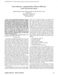
Fig. 1. Mean values and the 95% CI of the estimated SOI and noise powers obtained via (a) NLS, (b) DA, (c) IDA, and (d) ML using simulated data with .
M=8
where and and setting to zero, we have of
. Taking the derivative (30)
or equivalently (25) is the real part of . The solution of (25) where without the nonnegative constraint is the eigenvector corresponding to the smallest eigenvalue of , i.e., . Hence, if , then is the final solution of (25) (or , then is the solution); otherwise, if the optimization problem in (25) is hard to solve exactly and we approximate as one of the following two vectors that gives the smaller value of the cost function in (25):
(26) In this way, we get an estimate of within a multiplicative constant. Next, we need to estimate the scaling factor . We insert the initial estimate into (16) and (17) and then average (16) over and (17) over and ( ) to get (27) where
, ,
, , and
. By removing the parameter , which depends on , we have the following equation from (27): (28) Since , and are real-valued scalars, while and are complex-valued scalars, the exact solution of (28) might not exist. Alternatively, we solve the following equation to get :
(29)
There are three roots for (30) and we need to select a root such that is real-valued and nonnegative. If more than one root satisfy the aforementioned criteria, we choose the one that gives the smallest value of , which is the particular root that satisfies (29). After we obtain , and thus the final estimate of as , we can estimate by the following equation (see [5] for details): (31) where and denote the dominant eigenvalue and eigenvector of a matrix, respectively. The procedure of the IDA method can be summarized as follows. Step 1) Compute and then by (23). and then . Step 2) Obtain Step 3) Obtain the initial estimate by (25). Step 4) Compute the scaling factor by (30) and then the final estimate . Step 5) Compute by (31) and then estimate the SOI power as . IV. EXAMPLES We first present several numerical examples to evaluate the proposed methods. For reference, the results of the existing NLS algorithm (see [4]) and the ML method (ML is based on the maximum likelihood algorithm and gives the best performance among the proposed methods in [5]) are also included. We assume that eight microphones ( ) are available in the system. The vectors are generated as independent and identically distributed (i.i.d.) zero-mean circularly symmetric complex Gaussian random vectors with covariance matrix , where the true power levels for the SOI ( ) and the noise ( ) are denoted by the circles in Fig. 1, and the phases of are chosen independently from uniform distribution between 0 and . Fig. 1 shows the mean values and the 95% confidence interval (95% CI, shown as the small bars around the mean values) of power estimates for various algorithms obtained from 1000
14
IEEE SIGNAL PROCESSING LETTERS, VOL. 18, NO. 1, JANUARY 2011
0
Fig. 2. MSEs of the SOI power estimates for Microphone 4 (SNR = 25 dB) = 8. Computation and the corresponding CRB using simulated data with time: NLS (39 min 26 s); DA (24 s); IDA (26 s); ML (2 min 2 s).
M
Monte-Carlo trials, along with the true powers at each micro. As phone. The number of data samples is set to shown in the plots, ML gives the best performance in all cases and IDA performs similarly to ML. While DA gives worse performance than ML and IDA, it provides much more accurate power estimates than NLS for microphones 4, 5 and 6, where SNR is relatively low. For further examination, we show the mean square errors (MSEs) of the SOI power estimates obtained from 1000 MonteCarlo trials as well as the corresponding Cramér-Rao Bounds for micro(CRB) as a function of the data sample number phone 4 (with the lowest ). The details for the derivations of CRB can be found in [5]. The results are shown in Fig. 2 (based on the results and those for the other microphones, sample size over 1000 is sufficient for the proposed algorithms to provide reliable results). Note that ML converges to CRB for large , which is as expected since ML is asymptotically statistically efficient for a large number of data samples. IDA gives the second best performance, followed by DA. NLS provides the poorest results. The total computation time of this example for each method is given in the figure caption, which is obtained using a PC with CPU Core(TM)2 Duo E6850 (3 GHz). As evidenced, DA is computationally the most efficient method, and IDA is comparable to it. ML takes almost four times longer to run than those two, while NLS demands much more computation time. Next, we use experimental trailing edge noise data to evaluate the new methods. The data was obtained from a NACA 63–215 Mod B airfoil at the University of Florida Aeroacoustic Flow Facility (see [4], [5] for the experimental setup). The specific data set is the same one as used in [5]. A total of 12 microphones were used to record the measurement, while the data acquired by the two microphones close to the jet collector are not used in the present analysis because the microphones experienced severe hydrodynamic pressure fluctuations [5]. The sampling rate was set to 32.768 KHz, and the length of each data block was 2048, resulting in a 16 Hz narrowband frequency bin. A Hanning window with 75% overlap is applied to each block, leading to 996 effective block averages in the construction of the sample covariance matrix . Fig. 3 shows the SOI power estimates obtained via all the algorithms as a function of the frequency for microphone 5 (the one right below the trailing edge).
Fig. 3. SOI power spectrum estimates for Microphone 5 using the measured data. Computation time: NLS (5 min 8 s); DA (0.1 s); IDA (0.4 s); ML (22 s).
For lower frequencies, the proposed methods (DA and IDA) and ML behave similarly in most cases, and have somewhat divergent trends from NLS (e.g., near 1800 Hz). All methods break down near 3500 Hz. A reasonable explanation is that for frequency larger than 3500 Hz, additional wind-tunnel facility noise, distributed in space and partially correlated in nature, begins to dominate the trailing edge noise signal, thus violating the assumptions made for this analysis [5]. We also compare the computation time of this example for all methods. Again, DA and IDA are much faster than ML and NLS (more than 50 times faster than ML and 750 times faster than NLS). V. CONCLUSIONS Two computationally efficient techniques, namely DA and IDA, have been presented for aeroacoustic source power estimation. The algorithms have been evaluated and compared with each other and with the existing NLS and ML methods using both simulated and measured data. In the numerical examples, the proposed algorithms, especially IDA, have been shown to provide accurate SOI power estimates even under low SNR conditions. Experimental examples show that the SOI power estimates obtained using the proposed algorithms are consistent with each other and the existing algorithms. Furthermore, we have shown that the proposed algorithms are computationally much more efficient than ML and NLS. REFERENCES [1] F. V. Hutcheson and T. F. Brooks, “Measurement of trailing edge noise using directional array and coherent output power methods,” in 8th AIAA/CEAS Aeroacoustics Conf., Breckenridge, CO, Jun. 2002, AIAA-2002-2472. [2] T. F. Brooks and T. H. Hodgson, “Trailing edge noise prediction from measured surface pressures,” J. Sound Vibr., vol. 78, no. 1, pp. 69–117, 1981. [3] J. S. Bendat and A. G. Piersol, Random Data Analysis and Measurement Procedures, 3rd ed. New York: Wiley, 2000. [4] C. Bahr, T. Yardibi, F. Liu, and L. Cattafesta, “An analysis of different measurement techniques for airfoil trailing edge noise,” in 14th AIAA/CEAS Aeroacoustics Conf., Vancouver, BC, Canada, May 2008, AIAA-2008-2957. [5] L. Du, L. Xu, J. Li, B. Guo, P. Stoica, C. Bahr, and L. Cattafesta, “Covariance-based approaches to aeroacoustic noise source analysis,” J. Acoust. Soc. America, 2010, to be published. [6] P. Stoica and R. L. Moses, Spectral Analysis of Signals. Upper Saddle River, NJ: Prentice-Hall, 2005.