Computationally Efficient Micromechanical Models for ...

R. Tanov Graduate Research Assistant

A. Tabiei1 Assistant Professor and Director Center for Excellence in DYNA3D Analysis, Department of Aerospace Engineering and Engineering Mechanics, Uiniversity of Cincinnati, Cincinnati, OH 45221-0070

1

Computationally Efficient Micromechanical Models for Woven Fabric Composite Elastic Moduli This paper presents two newly developed micromechanical models for the analysis of plain weave fabric composites. Both models utilize the representative volume cell approach. The representative unit volume of the woven lamina is divided into subcells of homogeneous material. Starting with the average strains in the representative volume cell and based on continuity requirements at the subcell interfaces, the strains and stresses in the composite fiber yarns and matrix are determined as well as the average stresses in the lamina. Equivalent homogenized material properties are also determined. In their formulation the developed micromechanical models take into consideration all components of the three-dimensional strain and stress tensors. The performance of both models is assessed through comparison with available results from other numerical, analytical, and experimental approaches for composite laminae homogenization. The very good accuracy together with the simplicity of formulation makes these models attractive for the finite element analysis of composite laminates. 关DOI: 10.1115/1.1357516兴

Introduction

Composite laminae are being more and more extensively utilized in modern shell structures. High specific stiffness, specific strength, and toughness are among their advantageous properties, which make composite shells the preferred choice in all kinds of aerospace, automotive, and marine vehicles, industrial, civil and other structures. Of the two major types of composite laminae, woven fabric composites have long been recognized as more competitive than unidirectional composites. This is partly due to their ability to provide good reinforcement in all directions within a single layer, to their better impact resistance, better-balanced properties, easier handling and fabrication, and good ability to conform to surfaces with complex curvatures. Along with that, however, their complex architecture makes the analysis of their behavior much more challenging. Therefore, it is not surprising that there are substantialy fewer approaches for determining the properties of woven fabric laminae and predicting their behavior than for unidirectional composites. Most of them utilize the representative unit cell approach—the properties and behavior of the entire lamina are considered to be the same as the properties of a unit cell. The entire complex geometry of the composite layer can usually be reproduced by using this representative volume cell 共RVC兲 as a building block. Earlier models for the analysis of woven fabric composites include the works of Ishikawa and Chou 关1– 4兴, who developed three different models: the mosaic model, the fiber-undulation model, and the bridging model. The mosaic model is based on the classical lamination theory and represents the woven composite as an assemblage of asymmetrical cross-ply laminates. Using the isostress 共or series model兲 and iso-strain 共or parallel model兲 assumptions, the upper and lower bounds of the elastic moduli can be 1 To whom author should be addressed. Contributed by the Applied Mechanics Division of THE AMERICAN SOCIETY OF MECHANICAL ENGINEERS for publication in the ASME JOURNAL OF APPLIED MECHANICS. Manuscript received by the ASME Applied Mechanics Division, April 18, 2000; final revision, October 24, 2000. Associate Editor: M-J. Pindera. Discussion on the paper should be addressed to the Editor, Professor Lewis T. Wheeler, Department of Mechanical Engineering, University of Houston, Houston, TX 77204-4792, and will be accepted until four months after final publication of the paper itself in the ASME JOURNAL OF APPLIED MECHANICS.

Journal of Applied Mechanics

derived with this model. The fiber-undulation model takes into account the fiber undulation and continuity. Both the mosaic and the fiber-undulation models are one-dimensional models. The bridging model was developed for the analysis of satin composites. In this model the regions with straight threads are assumed to act as load-carrying bridges between adjacent interlaced regions. Naik and Shembekar 关5兴 developed two-dimensional micromechanical models using the parallel-series assumptions. These models are based on the classical lamination theory assuming that it is applicable to each infinitesimal piece of the RVC. The models are capable of describing the RVC geometry in detail, including the fiber yarn cross sections and the undulated portions, and can be used to determine the homogenized in-plane stiffness properties of the RVC. Karayaka and Kurath 关6兴 used the RVC approach to develop a micromechanical model capable of representing both plain weave and satin weave composite layers. The model is based on the assumption that all in-plane strain and out-of-plane stress components are constant throughout the RVC. It was used in 共关6兴兲 to investigate the behavior of a five-harness satin weave Graphite/ Epoxy laminate. Tabiei and Jiang 关7兴 developed a micromechanical model, which considers the two-dimensional extent of woven fabric laminae and is based on nonlinear stress-strain relations. Within this model the RVC is divided into many subcells and an averaging is performed to obtain the effective stress-strain relations. This model is suitable for implementation into nonlinear finite element codes to enable structural analyses of woven composites. Recently, Tabiei et al. 关8兴 presented a nonlinear constitutive model for plain weave composites. The incremental constitutive model was developed based on micromechanics. This model considers material nonlinear behavior of both resin and fill/warp yarns. A global/local approach to woven metal matrix composites analysis was developed by Bednarcyk and Pindera 关9,10兴. The approach uses a local unidirectional micromechanical model to represent the fibers and matrix, which constitute the fiber yarns, and a three-dimensional global model to simulate the overall behavior of the RVC. This approach is used to predict the response of eight-harness satin weave Carbon/Copper composites and compare the results to experimental data.

Copyright © 2001 by ASME

JULY 2001, Vol. 68 Õ 553

Along with the analytical models of woven fabric composites there are also some numerical approaches utilizing the finite element method. Using a three-dimensional model, Whitcomb 关11兴 analyzed a RVC of a plain weave composite. Whitcomb used his finite element model to assess the influence of different parameters on the stiffness properties of the RVC. In their work Chung and Tamma 关12兴 summarize and compare various homogenization methods via finite element analyses. The aim of the present work is to develop micromechanical models for plain weave composites, which could be incorporated efficiently into explicit and implicit finite element codes to be able to perform structural analysis of composite and sandwich shells with woven fabric layers. This will enable determination of the state of stress and strain in the constituent fiber yarns and matrix within the finite element analysis, which could be used to perform material failure and property degradation checks within the structural analysis process. Many of the presently existing analytical models lack either accuracy or efficiency or both, to be capable of providing the above features to a finite element analysis. The finite element models usually have a good accuracy and are capable of correctly modeling the three-dimensional state of stress and strain in the RVC and its constituents, but involve too many elements in discretizing the RVC to be used for composite structural analysis. The analytical model of Tabiei and Jiang described in 共关7兴兲 proved efficient for an implicit finite element analysis, but the nature of the explicit time integration scheme will make it hard to fit into an explicit finite element analysis code. To a certain degree, this also applies to one of the herein presented models, namely the single-cell model. However, the other model described here, the four-cell model, solves only a small system of six linear equations, which would make it much more efficient in an explicit finite element analysis. In what follows two new micromechanical models are formulated and their performance is checked and compared with results from other numerical, analytical, and experimental approaches employed in the analysis of plain weave fabric composites.

2

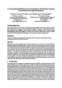
Fig. 1 Plain weave architecture, representative volume cell, and one quarter cell

the strain and stress tensors, and starting with the strains in the RVC are capable of determining the three-dimensional constitutive matrix of the homogenized RVC and all stress and strain components in the composite constituents. Both models assume that the RVC is assembled using certain number of subcells, which are under homogeneous state of stress and strain. The following assumptions are also used in the models: 共a兲 the matrix is isotropic and the yarn fiber bundles are transversely isotropic with principal axis along the yarn axis; 共b兲 the contact between the constituents is perfect, i.e., displacements and traction are continuous across the constituent contact interfaces. Both formulations are developed with the intention to be used in a finite element composite shell analysis. Therefore, in the formulations, the average strains within the RVC are assumed to be available, which is the case in a standard displacement based finite element analysis. The models are then used to find the strains and stresses in the composite constituents, and the average stresses in the entire RVC or the tangent stiffness matrix. If 关 C兴 m and 关 C兴 y are the constitutive matrices of the matrix and yarn in a material local coordinate system then

Formulation of the Micromechanical Models

Both models developed and described in this work utilize the RVC approach 共see Fig. 1兲. In that the authors have tried to achieve an optimal balance between the two major parts of the formulation: the geometric description of the RVC, and the micromechanical representation of the developed model. This is something that many existing models lack; a tedious formulation is used to describe the RVC geometry with a very high precision, and at the same time the accuracy of that geometric description cannot be taken advantage of due to overly simplified micromechanical descriptions. This makes these approaches hard to implement in a real world analysis and at the same time the accuracy of the acquired results often does not match the solution effort needed. The geometric description of the RVC in the present models is much simpler compared to other approaches 共e.g., see Naik and Shembekar 关5兴兲, which translates into computational efficiency and easy implementation. Yet, as the herein presented results show, their accuracy is very good for different values of the RVC geometric and material parameters. An important contribution for this accuracy is due to the three-dimensional micromechanical description of the RVC. Previous micromechanical models implement two-dimensional 共Naik and Shembekar 关5兴兲 and even one-dimensional 共Ishikawa and Chou 关1–4兴兲 approaches in the RVC description, which can significantly affect the solution accuracy. In the present approaches the entire woven fabric lamina can be constructed by using the RVC, Fig. 1共b兲, as a building block. Assuming that the fiber yarns in both direction 共the fill and warp兲 have the same structure and properties, the entire RVC, Fig. 1共b兲, can be constructed by using just one quarter of it, Fig. 1共c兲, and this quarter cell is hereafter referred to as the RVC. In their formulation the models described here consider all components of 554 Õ Vol. 68, JULY 2001

关 C兴 m ⫽

where Cm 11⫽

冤

Cm 11

Cm 12

Cm 12

0

0

0

Cm 12 Cm 12

Cm 11 Cm 12

Cm 12 Cm 11

0

0

0

0

0

0

0

0

Cm 44

0

0

Cm 44

0

0

0

Cm 44

0

0

0

0

0

0

0

E m 共 1⫺ ␯ m 兲 ; 共 1⫹ ␯ m 兲共 1⫺2 ␯ m 兲 Cm 44⫽G m ⫽

0

Cm 12⫽

冥

,

(1)

E m␯ m 共 1⫹ ␯ m 兲共 1⫺2 ␯ m 兲

Em 2 共 1⫹ ␯ m 兲

;

(2)

and E m , ␯ m , and G m are the matrix Young’s modulus, Poisson’s ratio, and shear modulus, respectively. Both fill and warp yarns are assumed to be of the same fiber material, with constitutive matrix of the yarns

关 C兴 y ⫽

where

冤

y C 11

y C 12

y C 12

0

0

0

y C 12 y C 12

y C 22 y C 23

y C 23 y C 22

0

0

0

0

0

0

0

y C 44

0

0

0

0

0

0

0

0

0

0

0

0

y y C 22 ⫺C 23

2 0

0 y C 44

冥

,

(3)

Transactions of the ASME

y C 11 ⫽

E v ,L 共 1⫺ ␯ 2y,TT 兲 ⌬ y C 22 ⫽

y C 23 ⫽

;

y C 12 ⫽

E y,T ␯ y,LT 共 1⫹ ␯ y,TT 兲 ; ⌬

E v ,T 共 1⫺ ␯ y,LT ␯ y,TL 兲 ; ⌬

E y,T 共 ␯ y,TT ⫹ ␯ y,LT ␯ y,TL 兲 ; ⌬

(4)

y C 44 ⫽G y,LT ;

⌬⫽1⫺ ␯ 2y,TT ⫺2 ␯ y,LT ␯ y,TL 共 1⫹ ␯ y,TT 兲 . Here ␯ y,TL ⫽ ␯ y,LT (E y,T /E y,L ) and E y,L ,E y,T , ␯ y,LT , ␯ y,TT ,G y,LT are the Young’s moduli, Poisson’s ratios, and the shear modulus of the transversely isotropic yarn; subscripts L and T denote the direction along the yarn axis and the transverse to it direction, respectively. Note that in the above formulas the commas in the subscripts do not represent differentiation. The above constitutive matrices, Eqs. 共1兲 and 共3兲, relate the stress and strain tensor components arranged in vectors as follows:

兵 ␴其 ⫽ 兩 ␴ x ␴ y ␴ z ␴ xy ␴ yz ␴ zx 兩 T ; 兵 ␧其 ⫽ 兩 ␧ x ␧ y ␧ z ␥ xy ␥ yz ␥ zx 兩 T ,

(5)

with ␥ i j ⫽2␧ i j being the engineering shear strains. A description of the geometry and mechanics of the models follows. Since in the first model we divide the quarter cell into four subcells in the lamina plane it will be referenced here as ‘‘the four-cell model,’’ while the second model, which has only one cell in the lamina plane will be referenced as ‘‘the single-cell model.’’ 2.1

The Four-Cell Model

2.1.1 Geometry of the Model. The geometry of this model is shown in Fig. 2共a兲. To keep the formulation simple, the cross sections of the fill and warp yarns are assumed rectangular and their undulating form is approximated with only horizontal and inclined at angle ␪ sections, ␪ being the average undulation angle. This representation makes it possible to divide the RVC into four subcells, denoted by ‘‘ff,’’ ‘‘fm,’’ ‘‘mm,’’ and ‘‘mf’’ on Fig. 2共a兲. Subcell ‘‘ff’’ is further divided into two sub-subcells, Fig. 2共b兲, which represent the horizontal portions of the two yarns. Subcells ‘‘fm’’ and ‘‘mf’’ consist of yarn and matrix portions as illustrated on Fig. 2共c兲. Each one of them contains half of the inclined portion of the yarns; by putting two such subcells together we get the entire undulated portion of the yarn. Subcell ‘‘mm’’ is entirely of matrix material. Let us assume that the RVC has height of H units and sides of length one unit each. Then, if both yarns have a rectangular cross section with sides H/2 and V y , V y being the overall yarn volume fraction, the ratio of the volume of the yarns to the volume of the entire RVC will equal V y . Furthermore, the undulation angle, ␪, can also be expressed through the total RVC height, H, and the yarn volume fraction, V y from tan ␪ ⫽

H . 4 共 1⫺V y 兲

(6)

Thus, only two parameters, namely H and V y , or ␪ and V y are sufficient to completely define the geometry of the RVC. Furthermore, the dimensions of the sub-subcells are also completely defined with these two parameters. Note that in the present formulation this model does not include a layer of matrix material, which covers the entire RVC. Therefore, the height of the yarns is half the thickness of the entire lamina. If the real lamina to be represented by this model has a matrix layer of significant thickness then the model can be modified to include it, which would not change the basis of the formulation. 2.1.2 Micromechanics of the Model. Within the subcells ‘‘ff,’’ ‘‘mf,’’ and ‘‘fm’’ the constituent yarn and matrix materials are first combined to get an equivalent homogeneous material in each subcell 共subcell ‘‘mm’’ is entirely matrix so there is no need to homogenize it兲. The four subcells are then combined to get an equivalent homogeneous RVC. The homogenization is based on the parallel-series assumptions: For some of the strain components the adjacent cells are assumed to work ‘‘in parallel’’ and the corresponding strains are equal; for the rest of the strains, the cells are assumed to work ‘‘in series’’—the corresponding stress components are equal and the strain components are averaged to get the entire cell resultant strains. Similar assumptions are used as a basis for many micromechanical models for unidirectional and woven composites. The homogenization of the subcells ‘‘ff’’ and ‘‘mf’’ is described in the following. 2.1.2.1 Homogenization of subcell ‘‘ff’’. The subcell ‘‘ff’’ is shown on Fig. 2共b兲. It consists of two homogeneous parts of equal thickness, top fill and bottom warp. Both of them are of the same transversely isotropic material with axis of transverse isotropy along the corresponding yarn axis, which is x for the fill and y for the warp. So, the fill and warp constitutive matrices will be as follows:

关 C兴 fill⫽

and

冤 冤

关 C兴 warp⫽

y C 11

y C 12

y C 12

0

0

0

y C 12 y C 12

y C 22 y C 23

y C 23 y C 22

0

0

0

0

0

0

0

0

y C 55

0

0

y C 44

0

0

0

y C 44

0

0

0

0

0

0

0

y C 22

y C 12

y C 23

0

0

0

y C 12 y C 23

y C 11 y C 12

y C 12 y C 22

0

0

0

0

0

0

0

0

0

0

0

y C 44

0

0

0

0

y C 44

0

0

0

0

0

0

y C 55

Journal of Applied Mechanics

(8)

y y y with C 55 ⫽C 22 ⫺C 23 /2. Assuming we have available the homogeneous strain tensor components, ␧ if jf , of the entire subcell ‘‘ff,’’ we will express the strains and stresses in the fill and warp portions, and the stresses in the entire subcell. From the perfect contact and the parallelseries assumption we have at the fill-warp interface:

␧ xf f ⫽␧ xf ⫽␧ wx

Fig. 2 Geometry of the quarter cell for the four-cell model

0

冥 冥

(7)

␴ zf f ⫽ ␴ zf ⫽ ␴ zw

␧ yf f ⫽␧ yf ⫽␧ wy

ff f ␴ yz ⫽ ␴ yz ⫽ ␴ wyz

ff f w ␧ xy ⫽␧ xy ⫽␧ xy

ff f w ␴ zx ⫽ ␴ zx ⫽ ␴ zx

(9) .

Here a single superscript f is used to denote that the corresponding quantity refers to the fill yarn, and w refers to the warp yarn. JULY 2001, Vol. 68 Õ 555

The rest of the strain and stress tensor components of the subcell are assumed volume averages of the strains and stresses of the constituent fill and warp parts:

␴ xf f ⫽ 21 共 ␴ xf ⫹␧ wx 兲

1

␧ zf f ⫽ 2 共 ␧ zf ⫹␧ zw 兲

␴ yf f ⫽ 21 共 ␴ yf ⫹ ␴ wy 兲

ff f ␧ yz ⫽ 21 共 ␧ yz ⫹␧ wyz 兲

(10)

1 ff f w ␴ xy ⫽ 2 共 ␴ xy ⫹␧ xy 兲.

1 ff f w ␧ zx ⫽ 2 共 ␧ zx ⫹␧ zx 兲

Note that the above relations combined with the assumption of homogeneous strains and stresses within the subcells will result in violation of the displacement continuity with respect to the surrounding subcells. Therefore, the values of the strains in the subcell should be treated as subcell average values, satisfying the displacement continuity in an average sense. Using the above equations, Eqs. 共9兲 and 共10兲, the unknown strain components in the fill and warp parts can be expressed: ␧ zf ⫽␧ zf f ⫺

y y C 12 ⫺C 23 共 ␧ xf f ⫺␧ yf f 兲 y 2C 22 f ␧ yz ⫽

f ␧ zx ⫽

y 2C 44 y y C 44 ⫹C 55

␧ zw ⫽␧ zf f ⫹

ff ␧ yz ␧ wyz ⫽

y 2C 55

ff y y ␧ zx C 44 ⫹C 55

w ␧ zx ⫽

ff C 12 ⫽

冋 冋

y 2C 55 y y C 44 ⫹C 55

ff ␧ yz

ff y y ␧ zx C 44 ⫹C 55

y y 2 ⫺C 23 兲 共 C 12 y 2C 22

ff ff C 13 ⫽C 23 ⫽

.

册

册

These values of the strains in the yarn local coordinate system will only be needed if the strains and stresses in the matrix and fill parts are needed. If not, the homogenized subcell constitutive matrix constructed below can be directly used to get the subcell average stresses in the RVC global coordinate system. The yarn local coordinate system, x ⬘ y ⬘ z ⬘ , can be obtained by rotating the RVC global coordinate system around the y-axis at an angle ␪. The variables expressed in that coordinate system will be denoted by a superscript prime. In that coordinate system, similar relations to Eqs. 共9兲 and 共10兲 should hold:

mf f m 兲 ⬘ ⫽ 共 ␧ xy 兲 ⬘ ⫽ 共 ␧ xy 兲⬘ 共 ␧ xy

2

(12)

1

f f m 共␧m yz 兲 ⬘ ⫽ 2 关共 ␧ yz 兲 ⬘ ⫹ 共 ␧ yz 兲 ⬘ 兴 1

y y C 44 ⫹C 55

.

mf f m 兲 ⬘ ⫽ 2 关共 ␧ zx 兲 ⬘ ⫹ 共 ␧ zx 兲⬘兴 共 ␧ zx 1

ff C 12

ff C 13

0

0

0

ff C 12

ff C 11

ff C 13

0

0

0

ff C 13

ff C 13

ff C 33

0

0

0

0

0

0

ff C 44

0

0

0

0

0

0

ff C 55

0

0

0

0

0

0

ff C 55

冥

共 ␴ zm f 兲 ⬘ ⫽ 共 ␴ zf 兲 ⬘ ⫽ 共 ␴ zm 兲 ⬘ f f m 共␴m yz 兲 ⬘ ⫽ 共 ␴ yz 兲 ⬘ ⫽ 共 ␴ yz 兲 ⬘

(15)

mf f m 兲 ⬘ ⫽ 共 ␴ zx 兲 ⬘ ⫽ 共 ␴ zx 兲⬘ 共 ␴ zx

and 共 ␧ zm f 兲 ⬘ ⫽ 2 关共 ␧ zf 兲 ⬘ ⫹ 共 ␧ zm 兲 ⬘ 兴

ff C 11

f f m 共␴m x 兲 ⬘ ⫽ 2 关共 ␴ x 兲 ⬘ ⫹ 共 ␴ x 兲 ⬘ 兴 1

f f y 共␴m y 兲 ⬘ ⫽ 2 关共 ␴ y 兲 ⬘ ⫹ 共 ␴ m 兲 ⬘ 兴 (16) 1

mf f m 兲 ⬘ ⫽ 2 关共 ␴ xy 兲 ⬘ ⫹ 共 ␴ xy 兲⬘兴. 共 ␴ xy 1

From these relations we can determine the unknown strain components in the yarn local coordinate system in the matrix and fill parts, which are

.

(13)

Thus, the homogenization of subcell ‘‘ff’’ is complete and provided the average strains, ␧ if jf , in the subcell are known, all strains in stresses in the constituents can be determined, as well as the average subcell stresses. 2.1.2.2 Homogenization of subcells ‘‘mf’’ and ‘‘fm’’. Since subcells ‘‘mf’’ and ‘‘fm’’ have similar geometry, their constitutive matrices will be also similar and will be related through a simple coordinate rotation. Therefore, only the derivation of the 556 Õ Vol. 68, JULY 2001

mf f mf 兲 ⬘ ⫽2␧ m 共 ␥ zx x sin ␪ cos ␪ ⫺2␧ z sin ␪ cos ␪

f f m 共␧m y 兲⬘⫽共 ␧ y 兲⬘⫽共 ␧ y 兲⬘

Finally, the constitutive matrix of subcell ‘‘ff’’ is

冤

mf mf sin ␪ ⫹ ␥ myzf cos ␪ 兲 ⬘ ⫽ ␥ xy 共 ␥ xy

y y C 12 ⫹C 23

y y 2C 44 C 55

(14)

mf mf cos ␪ ⫺ ␥ myzf sin ␪ 兲 ⬘ ⫽ ␥ xy 共 ␥ xy

f f m 共␧m x 兲⬘⫽共 ␧ x 兲⬘⫽共 ␧ x 兲⬘

ff y C 44 ⫽C 44

关 C兴 f f ⫽

f mf mf 2 2 共 ␧ zm f 兲 ⬘ ⫽␧ m x sin ␪ ⫹␧ z cos ␪ ⫹ ␥ zx cos ␪ sin ␪

(11)

ff y ⫽C 22 C 33

ff ff C 55 ⫽C 66 ⫽

f mf 共␧m y 兲 ⬘ ⫽␧ y

mf ⫹ ␥ zx 共 cos2 ␪ ⫺sin2 ␪ 兲 .

y 2C 44

y y 2 ⫺C 23 兲 共 C 12 1 y y C 11⫹C 22 ⫺ y 2 2C 22

1 y 2C 12 ⫹ 2

f mf mf mf 2 2 共␧m x 兲 ⬘ ⫽␧ x cos ␪ ⫹␧ z sin ␪ ⫺ ␥ zx cos ␪ sin ␪

y y C 12 ⫺C 23 共 ␧ xf f ⫺␧ yf f 兲 y 2C 22

So, all strains in the constituents are obtained, and knowing the constitutive matrices of the yarns, we can further express the stresses in the constituent. Also, from Eqs. 共9兲 and 共10兲, the average stresses in the entire subcell can be expressed in term of the average strains of the subcell. Thus the elements of the constitutive matrix of the homogenized subcell can be found, ff ff C 11 ⫽C 22 ⫽

constitutive matrix for subcell ‘‘mf’’ will be shown, and the constitutive matrix for subcell ‘‘fm’’ will be derived using the appropriate transformation. Subcell ‘‘mf’’ contains matrix and yarn parts of equal volumes. If the undulation angle, ␪, is not zero the material local coordinate system of the fill yarn part will not coincide with the xyz coordinate system 共see Fig. 2共c兲兲. However, we can take advantage of the isotropy of the matrix material and homogenize the subcell in the yarn local coordinate system, and then transfer the thus acquired constitutive matrix in the global xyz coordinate system. For this purpose we need to transfer the subcell average strains from the RVC global to the yarn local coordinate system

共 ␧ zm 兲 ⬘ ⫽

1

y mf y m mf y 关 2C 22共 ␧ z 兲 ⬘ ⫹ 共 C 12⫺C 12 兲共 ␧ x 兲 ⬘ Cm 11⫹C 22 y mf ⫹ 共 C 23 ⫺C m 12 兲共 ␧ y 兲 ⬘ 兴

共 ␧ zf 兲 ⬘ ⫽

1

m mf y m mf y 关 2C 11共 ␧ z 兲 ⬘ ⫹ 共 C 12⫺C 12 兲共 ␧ x 兲 ⬘ Cm 11⫹C 22 y mf ⫺ 共 C 23 ⫺C m 12 兲共 ␧ y 兲 ⬘ 兴

共␧m yz 兲 ⬘ ⫽ m 兲⬘⫽ 共 ␧ zx

y 2C 55

f 共␧m yz 兲 ⬘

f 兲⬘⫽ 共 ␧ yz

y 2C 44 mf m y 共 ␧ zx 兲 ⬘ C 44⫹C 44

f 兲⬘⫽ 共 ␧ zx

y Cm 44⫹C 55

(17) 2C m 44 y Cm 44⫹C 55

f 共␧m yz 兲 ⬘ .

2C m 44 mf m y 共 ␧ zx 兲 ⬘ . C 44⫹C 44

Transactions of the ASME

The constitutive matrix elements of the subcell in the x ⬘ y ⬘ z ⬘ coordinate system are

冋

y 2 ⫺C m 共 C 12 1 m 12 兲 f y C 11⫹C 11 ⫺ 共Cm m y 11 兲 ⬘ ⫽ 2 C 11⫹C 22 f 共Cm 12 兲 ⬘ ⫽

冋

y y m ⫺C m 共 C 12 1 m 12 兲共 C 23⫺C 12 兲 y C 12⫹C 12 ⫺ m y 2 C 11⫹C 22 f 共Cm 13 兲 ⬘ ⫽

f 共Cm 22 兲 ⫽

f 共Cm 23 兲 ⬘ ⫽

册

f mf mf Cm 26 ⫽ 关共 C 23 兲 ⬘ ⫺ 共 C 12 兲 ⬘ 兴 sin ␪ cos ␪

册

f 2 2 ⫹2 共 C m 66 兲 ⬘ 兴 sin ␪ cos ␪ f mf mf mf mf 2 2 Cm 36 ⫽ 兵 关共 C 13 兲 ⬘ ⫺ 共 C 11 兲 ⬘ 兴 sin ␪ ⫹ 关共 C 33 兲 ⬘ ⫺ 共 C 13 兲 ⬘ 兴 cos ␪ f 2 2 ⫺2 共 C m 66 兲 ⬘ 共 cos ␪ ⫺sin ␪ 兲 其 sin ␪ cos ␪

y Cm 11⫹C 22

冋

y 2 兲⫺共 Cm 共 C 23 1 m 12 兲 y C 11⫹C 22 ⫺ m y 2 C 11⫹C 22

f 共Cm 44 兲 ⬘ ⫽

f 共Cm 33 兲 ⬘ ⫽

f mf mf 2 2 Cm 44 ⫽ 共 C 44 兲 ⬘ cos ␪ ⫹ 共 C 55 兲 ⬘ sin ␪

册

f mf mf Cm 45 ⫽ 关共 C 55 兲 ⬘ ⫺ 共 C 44 兲 ⬘ 兴 sin␪ cos␪ f mf mf 2 2 Cm 55 ⫽ 共 C 44 兲 ⬘ sin ␪ ⫹ 共 C 55 兲 ⬘ cos ␪

(18)

y 2C 22 Cm 11 m y C 11⫹C 22

f mf mf mf 2 2 Cm 66 ⫽ 关共 C 11 兲 ⬘ ⫹ 共 C 33 兲 ⬘ ⫺2 共 C 13 兲 ⬘ 兴 sin ␪ cos ␪ f 2 2 2 ⫹共 Cm 66 兲 ⬘ 共 cos ␪ ⫺sin ␪ 兲 .

1 m y 兲 共 C ⫹C 44 2 44

y 2C 55 Cm 44

f 共Cm 66 兲 ⬘ ⫽

y Cm 44⫹C 55

y 2C 44 Cm 44 y Cm 44⫹C 44

The constitutive matrix of subcell ‘‘fm’’ can be obtained through an appropriate transformation of the above matrix, Eq. 共20兲 and is as follows:

.

Then, the constitutive matrix of subcell ‘‘mf’’ in the x ⬘ y ⬘ z ⬘ coordinate system is

⬘f 关 C兴 m

⫽

关 C兴 f m ⫽

冤

f 共Cm 11 兲 ⬘

f 共Cm 12 兲 ⬘

f 共Cm 13 兲 ⬘

0

0

0

f 共Cm 12 兲 ⬘ f 共Cm 13 兲 ⬘

f 共Cm 22 兲 ⬘ f 共Cm 23 兲 ⬘

f 共Cm 23 兲 ⬘ f 共Cm 33 兲 ⬘

0

0

0

0

0

0

0

0

0

f 共Cm 44 兲 ⬘

0

0

0

0

0

0

f 共Cm 55 兲 ⬘

0

0

f 共Cm 66 兲 ⬘

0

0

0

0

冥

(19)

By rotating back the local coordinate system x ⬘ y ⬘ z ⬘ at angle ␪ we will get the RVC global coordinate system. Transforming the above constitutive matrix, Eq. 共19兲, accordingly, will give us the subcell ‘‘mf’’ constitutive matrix in RVC global coordinate system, which is

关 C兴 m f ⫽

where

冤

f Cm 11 f Cm 12 f Cm 13

f Cm 12 f Cm 22 f Cm 23

f Cm 13 f Cm 23 f Cm 33

0

0

0

0

0

0

0

0

0

f Cm 44

f Cm 45

0

f Cm 55

0

0

f Cm 66

0

0

0

f Cm 45

f Cm 16

f Cm 26

f Cm 26

0

f Cm 16 f Cm 26 f Cm 36

冥

f mf mf mf 4 4 Cm 11 ⫽ 共 C 11 兲 ⬘ cos ␪ ⫹ 共 C 33 兲 ⬘ sin ␪ ⫹2 关共 C 13 兲 ⬘ f 2 2 ⫹2 共 C m 66 兲 ⬘ 兴 sin ␪ cos ␪ f mf mf 2 2 Cm 12 ⫽ 共 C 12 兲 ⬘ cos ␪ ⫹ 共 C 23 兲 ⬘ sin ␪ f mf mf 4 4 Cm 13 ⫽ 共 C 13 兲 ⬘ 共 cos ␪ ⫹sin ␪ 兲 ⫹ 关共 C 11 兲 ⬘ f mf 2 2 ⫹共 Cm 33 兲 ⬘ ⫺4 共 C 66 兲 ⬘ 兴 sin ␪ cos ␪ f mf mf mf mf 2 2 Cm 16 ⫽ 兵 关共 C 13 兲 ⬘ ⫺ 共 C 11 兲 ⬘ 兴 cos ␪ ⫹ 关共 C 33 兲 ⬘ ⫺ 共 C 13 兲 ⬘ 兴 sin ␪ f 2 2 ⫹2 共 C m 66 兲 ⬘ 共 cos ␪ ⫺sin ␪ 兲 其 sin ␪ cos ␪ f mf Cm 22 ⫽ 共 C 22 兲 ⬘

Journal of Applied Mechanics

(21)

f mf mf mf 4 4 Cm 33 ⫽ 共 C 11 兲 ⬘ sin ␪ ⫹ 共 C 33 兲 ⬘ cos ␪ ⫹2 关共 C 13 兲 ⬘

y m y C 12 Cm 11⫹C 12C 22

y m y C 23 Cm 11⫹C 12C 22 m y C 11⫹C 22

f 共Cm 55 兲 ⬘ ⫽

f mf mf 2 2 Cm 23 ⫽ 共 C 12 兲 ⬘ sin ␪ ⫹ 共 C 23 兲 ⬘ cos ␪

冤

0

f ⫺C m 26

0

f Cm 13 f Cm 33

0

0

0

f ⫺C m 16 f ⫺C m 36

0

f ⫺C m 45

f Cm 66

0

0

f Cm 55

f Cm 22

f Cm 12

f Cm 23

f Cm 12 f Cm 23

f Cm 11 f Cm 13

0

0

0

f Cm 44

f ⫺C m 26

f ⫺C m 16

f ⫺C m 36

0

0

f ⫺C m 45

0

0

0

冥

.

(22)

.

Thus, each subcell has been homogenized and its equivalent constitutive properties are available. The strains and stresses in the constituents, and the subcell resultant stresses can be determined, provided that the strains of the subcells are available. We can apply a similar parallel-series approach to the entire RVC and thus determine the strains in the subcells. Let us assume that the average strains in the RVC, ¯␧ i j , are available. Then, based on the parallel-series assumptions, the following relations will hold: For strains: f V y ␧ xf f ⫹ 共 1⫺V y 兲 ␧ m ¯x x ⫽␧

V y ␧ xfm ⫹ 共 1⫺V y 兲 ␧ mm ¯x x ⫽␧

V y ␧ yf f ⫹ 共 1⫺V y 兲 ␧ yfm ⫽␧ ¯y

V y ␧ my f ⫹ 共 1⫺V y 兲 ␧ mm ¯y y ⫽␧

␧ zf m ⫽␧ zmm ⫽␧ zf f ⫽␧ zm f ⫽␧ ¯z

(23)

fm mm ff mf ␧ xy ⫽␧ xy ⫽␧ xy ⫽␧ xy ⫽␧ ¯ xy

(20)

fm 2 ff V y 共 1⫺V y 兲共 ␧ yz ⫹␧ myzf 兲 ⫹ 共 1⫺V y 兲 2 ␧ mm ¯ yz yz ⫹V y ␧ yz ⫽␧ fm mf mm ff V y 共 1⫺V y 兲共 ␧ zx ⫹␧ zx ⫹V 2y ␧ zx ⫽␧ ¯ zx 兲 ⫹ 共 1⫺V y 兲 2 ␧ zx

For stresses:

␴ xfm ⫽ ␴ mm x

␴ xf f ⫽ ␴ mx f

f mm V y ␴ xf f ⫹ 共 1⫺V y 兲 ␴ xfm ⫽V y ␴ m ␴x x ⫹ 共 1⫺V y 兲 ␴ x ⫽ ¯

␴ yf f ⫽ ␴ yfm

␴ my f ⫽ ␴ mm y

V y ␴ yf f ⫹ 共 1⫺V y 兲 ␴ my f ⫽V y ␴ yfm ⫹ 共 1⫺V y 兲 ␴ mm ␴y y ⫽¯ V y 共 1⫺V y 兲共 ␴ zf m ⫹ ␴ zm f 兲 ⫹ 共 1⫺V y 兲 2 ␴ zmm ⫹V 2y ␴ zf f ⫽ ¯␴ z

(24)

fm mf mm ff V y 共 1⫺V y 兲共 ␴ xy ⫹ ␴ xy ⫹V 2y ␴ xy ⫽ ¯␴ xy 兲 ⫹ 共 1⫺V y 兲 2 ␴ xy fm ff mf ␴ yz ⫽ ␴ mm ␴ yz yz ⫽ ␴ yz ⫽ ␴ yz ⫽ ¯ fm mm ff mf ␴ zx ⫽ ␴ zx ⫽ ␴ zx ⫽ ␴ zx ⫽ ¯␴ zx

JULY 2001, Vol. 68 Õ 557

These relations, Eqs. 共23兲 and 共24兲, have been derived based on the assumption that there is a perfect bonding between the subcells, and the assumption of homogeneous strain and stress in each subcell. For example, considering the transverse normal strain component, ␧ z , it is obvious that the above assumptions lead to an equality in its value for all subcells, as expressed in Eq. 共23兲. The same applies for the in-plane shear strain ␧ xy . Using these assumptions in the geometric representation of the RVC, Fig. 2共a兲, all of the above relations, Eqs. 共23兲 and 共24兲, can be easily derived. They contain enough information to be able to express the 24 unknown strain components for all subcells. This will be done by solving a system of 16 linear equations with 16 unknowns. Note that the ␧ xy and ␧ z strain components are readily available. Also, some simple manipulations lead to ␧ mm yz ⫽ mm ␧ zx ⫽

f f Cm ␧ yz ⫹V y C m ␧ xy 55 ¯ 45 ¯

␧ myzf ⫽

f m mf Cm 55 ⫹V y 共 C 44⫺C 55 兲 f f Cm ␧ zx ⫺V y C m ␧ xy 55 ¯ 45 ¯

f m mf Cm 55 ⫹V y 共 C 44⫺C 55 兲

fm ␧ zx ⫽

the RVC to be of a unit length, then the volume of the entire RVC will be equal to H t . The volume of the two yarns will be H/2 ⫹a 共Fig. 3兲. Then H ⫹a⫽V y H t 2 tan ␪ 1 ⫽

H⫽2V y H t

.

2.2

The Single-Cell Model

2.2.1 Geometry of the Model. The geometry of the singlecell model is shown on Fig. 3. The entire quarter cell is represented by a single cell, which has four layers: two matrix, one fill, and one warp. The layers will be denoted with m t , f, w, and m b for the top matrix, fill, warp, and bottom matrix, respectively. They are separated by inclined planes, defined by appropriate dimensioning and the angles ␪ 1 and ␪ 2 共Fig. 3兲. The undulating form of the yarns is represented by prisms with trapezoidal cross section, inclined at an angle ⫹ ␪ 1 or ⫺ ␪ 1 , ␪ 1 being the average undulation angle. Only two parameters are needed to describe the geometry of the entire RVC—the yarn volume fraction, V y , and the lamina thickness, H t . If we assume the in-plane dimensions of

Fig. 3 Geometry of the quarter cell for the single-cell model

558 Õ Vol. 68, JULY 2001

b⫽H t

(26)

冉 冊 1 ⫺V y 2

V yHt . 2

If V y ⬎0.5 we assume that b⫽0. Then H⫽H t

(25) This reduces the rank of the system of equations to 12. Furthermore, by using some of the simple relations in the equations the system of linear equations can be reduced to six equations with six unknown—the remaining strain components of the subcells. The coefficient matrix of this system is not fully populated, which makes it possible to explicitly express the six unknowns. After solving this system all strain components in the subcells will be available. Then with the values of these strains all strains and stresses in the fill, warp, and matrix parts of the subcells can be determined, as well as the average stresses in the subcells. These stress values can be finally used in Eq. 共24兲 to calculate the average stresses in the homogenized RVC. Thus, the micromechanical description of the RVC will be complete. As already stated this approach would result in violations of the physical continuity between the adjacent subcells. However, the continuity requirements are satisfied in an average sense.

H tan ␪ 2 ⫽ ⫺a. 4

tan ␪ 1 ⫽tan ␪ 2 ⫽

f m mf Cm 55 ⫹V y 共 C 44⫺C 55 兲

f m mf Cm 55 ⫹V y 共 C 44⫺C 55 兲

H t ⫺H 2

If V y ⭐0.5 we assume that a⫽0. Then

f Cm ␧ yz ⫺ 共 1⫺V y 兲 C m ␧ xy 44¯ 45 ¯

f Cm ␧ zx ⫹ 共 1⫺V y 兲 C m ␧ xy 44¯ 45 ¯

H 4

b⫽

tan ␪ 1 ⫽

Ht 4

冉

a⫽H t V y ⫺ tan ␪ 2 ⫽H t

1 2

(27)

冊

冉 冊

3 ⫺V y . 4

(28)

Note that the maximum yarn volume fraction that this model can represent is 0.75. Therefore, if it is higher, 0.75 will be used in the geometry description, Eq. 共28兲, and the actual value is used in the micromechanical calculations. This is not expected to affect significantly the accuracy of the model. Experiments with values higher than 0.75 showed that the homogenized properties from this model compare very well with the values predicted by the four-cell model. 2.2.2 Micromechanics of the Model. The micromechanic description of this model is quite straightforward. In addition to the assumptions listed at the beginning of Section 2 it is also assumed that the strains and stresses of the entire RVC are weighted averages of the strains and stresses of the four layers. Thus, for the average RVC strain components we have ¯␧ i j ⫽

1⫺V y m t Vy f m 共 ␧ i j ⫹␧ i j b 兲 ⫹ 共 ␧ i j ⫹␧ iwj 兲 . 2 2

(29)

Assuming that the RVC average strain components, ¯␧ i j , are known, the above relation represents six equations for the 24 unknown strain components ␧ ikj , where k⫽m t , f ,w,m b . In addition to these six relations we have six continuity and traction conditions at each interface between the adjacent layers. These are 18 relations, which together with the above, Eq. 共29兲, form a system of 24 equations of 24 unknowns, the strain components in the four layers. The interface relations, however, have to be expressed in a coordinate system defined by the orientation of the interface. Here, we assume that the fibers of the fill and warp yarns lie in the xz and yz-planes, respectively 共see Fig. 3兲. Therefore, if the interface coordinate system is defined in such a way that one axis lies in one of these planes, it will be a principal material axis for that yarn. Then, the interface coordinate system will be the principal coordinate system in which the transverse isotropy of the yarn is expressed and the constitutive matrix of the yarn in this coordinate system will be that defined in Eqs. 共3兲 and 共4兲 above. Such coordinate systems are defined for the three layer interfaces. For example, at the m t - f interface, to define the interface local coordinate system we first need to rotate the global coordinate system about the y-axis at an angle ␪ 1 and then rotate it about the x-axis at ␪ 2 . Although for the fill-warp interface the local x and y-axes cannot lie in the global xz and yz-planes if ␪ 1 ⫽0, we will assume that they are close enough to be able to use the principal constitutive matrices for both layers without having to transfer them in a nonprincipal coordinate system. Simple trigonometric relations Transactions of the ASME

would show that the angles between the local x and y-axes and the corresponding principal axes are negligibly small for any realistic value of H t . So, at each of the three layer interfaces we have the following relations, which should hold expressed in the local interface coordinate system: At interface m t - f : m

f

␧ x t ⫽␧ x ⬘

m

f

⬘

␧ y t ⫽␧ y ⬘

␴ z t ⫽ ␴ zf ⬘

␴ y tz ⫽ ␴ yf ⬘ z ⬘

m

⬘

m

f

␧ x ty ⫽␧ x ⬘ y ⬘ ⬘ ⬘

m

⬘

m

f

␴ z tx ⫽ ␴ z ⬘ x ⬘

⬘ ⬘

⬘ ⬘

(30)

At interface f -w: f

w

␧ x ⬘ ⫽␧ x ⬘

␴ zf ⬘ ⫽ ␴ zw⬘

f

w

␧ y ⬘ ⫽␧ y ⬘

␴ yf ⬘ z ⬘ ⫽ ␴ wy ⬘ z ⬘

f

w

␧ x ⬘ y ⬘ ⫽␧ x ⬘ y ⬘

␴ zf ⬘ x ⬘ ⫽ ␴ zw⬘ x ⬘

(31)

At interface w-m b : w

m

␧ x ⬘ ⫽␧ x b ⬘

m ␴ zw⬘ ⫽ ␴ z b ⬘

w

m

␧ y ⬘ ⫽␧ y b ⬘

m ␴ wy ⬘ z ⬘ ⫽ ␴ y bz ⬘ ⬘

w

m

␧ x ⬘ y ⬘ ⫽␧ x by

⬘ ⬘

m ␴ zw⬘ x ⬘ ⫽ ␴ z bx ⬘ ⬘

(32)

In the above relations, Eqs. 共30兲–共32兲, the local coordinate system is denoted with a superscript prime. Since the strains in the four layers are the primary unknowns, the stress relations have to be expressed through the strains by using the corresponding constitutive relations. Then, these relations have to be transferred into the RVC global coordinate system where the primary unknowns live. The transformation matrices from RVC global to interface local coordinate system can be expressed through the angles ␪ 1 and ␪ 2 as indicated above. Equations 共29兲–共32兲 form a system of 24 equations with 24 unknowns, the strains in the four layers in global RVC CS. After solving this system, the stresses in the layers have to be calculated. For that purpose, for the fill and warp layers, the constitutive matrices have to be transformed into RVC global coordinates by a simple rotation about the y and x-axis, respectively. Finally, the average stresses in the RVC are calculated by volume averaging the stresses in the four layers: ¯␴ i j ⫽

1⫺V f m t Vf m 共 ␴ i j ⫹ ␴ i j b 兲 ⫹ 共 ␴ if j ⫹ ␴ iwj 兲 . 2 2

(33)

Thus, all strain and stress components in the four cell layers and in the RVC are determined, provided that the strains of the RVC are known. Compared to the four-cell model the single-cell model has both different geometric and mechanical description. The geometry of this model would more accurately represent tightly woven composites where there is no 共or almost no兲 portion of the thickness entirely occupied by the matrix. Its micromechanical representation is relatively straightforward but would be more appropriate for implementation in an implicit finite element analysis scheme due to the fact that a system of 24 equations has to be solved at each time iteration step. The four-cell model representation requires only the solution of a system of six equations, which would make it very efficient for an explicit finite element scheme. It was actually implemented as a separate constitutive model into the nonlinear dynamic explicit finite element code DYNA3D and used there to model the behavior of sandwich shells with woven composite facings. Some results from this study can be found in Chapters 4 and 5 of 关13兴.

3

Table 1

Chung and Tamma 关12兴 used a finite element model to determine the elements of the homogenized constitutive matrix of a plain weave RVC. The RVC consists of epoxy matrix and fiber bundles, which are 65 percent E-glass/epoxy. The values for the material properties of the E-glass/epoxy yarns and the epoxy matrix are presented in Table 1. The overall fiber volume fraction is 0.35, but taking into account the 0.65 fiber volume fraction in the yarns, the yarn volume fraction that has to be used is V y ⫽0.35/0.65⫽0.5385. The average undulation angle determined approximately from the finite element model shown in 关12兴 is tan(␪)⫽1/6. The results for the RVC properties from upper and lower bound estimates from 关12兴 and from the present models are shown in Table 2. The results from 关12兴 were obtained by using prescribed displacement boundary conditions to get the upper bound, and prescribed stress boundary conditions to get the lower bound. As seen from this table, the results of both present models are good, the single-cell model being somewhat closer to the finite results from 关12兴. Table 3 presents results for the homogenized RVC material constants for the above-described case, and for the same RVC geometry with different materials shown in Table 1—Timetal␤21-S matrix and 65 percent SCS-6/Timetal yarns. The results from 关12兴 were acquired using the described there strain energy balance method, which gives an upper bound to the elastic constants. As seen, all values have very good agreement. Example 2 Results are compared with the finite element based micromechanical method of Marrey and Sankar 关14兴. The yarn is of Glass/ Epoxy with properties E L ⫽58.61 GPa, E T ⫽14.49 GPa, G LT ⫽5.38 GPa, ␯ LT ⫽0.250, ␯ TT ⫽0.247; the isotropic matrix is of Epoxy with E⫽3.45 GPa, ␯ ⫽0.37. The yarn volume fraction V y ⫽0.26, and from the RVC dimensions, the average undulation angle was estimated to be ␪ ⫽4.2 deg. The results from Reference 关14兴 are compared to the present results in Table 4. Some discrepancies of the values are probably due to the geometry of the

Table 2

Table 3

Results and Discussion

To test the performance of the two models presented here, several RVC’s with different constituent materials, yarn volume fractions, and undulation angles are homogenized and the results are compared to other published analytical, numerical, and experimental results. Example 1 Journal of Applied Mechanics

JULY 2001, Vol. 68 Õ 559

Table 4

composite layers, and will fit well into both explicit and implicit time integration schemes. Their very good accuracy was shown here through several tests, and together with the simplicity of formulation makes these models attractive for the finite element analysis of composite laminates.

Acknowledgments Table 5

The research within this study was supported by grant F4962098-1-0384 from the Airforce Office of Scientific Research. This support is gratefully acknowledged.

References

RVC—V y is low and there are entirely matrix layers on both sides of the lamina, as well as between the fill and warp. Both our models do not consider a matrix layer between the fill and warp, and in the present formulation of the four-cell model there are also no matrix layers on the outer sides of the lamina. Example 3 With this example the performance of the present models is compared to the micromechanical model of Tabiei and Jiang 关7兴, Jiang et al. 关15兴, and the experimental results of Ishikawa et al. 关16兴. The Graphite/Epoxy RVC is described in 共关15兴兲 and 共关16兴兲 and consists of yarns with properties E L ⫽137.3 GPa, E T ⫽10.79 GPa, G LT ⫽5.394 GPa, ␯ LT ⫽0.26, ␯ TT ⫽0.46, and isotropic matrix with E⫽4.511 GPa, ␯ ⫽0.38. The RVC parameters of the geometry are V y ⫽0.58, and ␪ ⫽1.4 deg. As seen from Table 5 the values of the moduli from the present approach are close to the analytical results from 共关15兴兲 and the experimental results from 共关16兴兲.

4

Conclusions

The micromechanical models developed in this study have relatively simple formulations, yet they provide very good accuracy of the results for the elastic properties for all examined cases. The new models are formulated based on three-dimensional representations, and thus consider all components of the strain and stress tensors. They can be used to determine the strains and stresses in the constituent fiber yarns and matrix of a plain weave composite, and to acquire homogenized constitutive properties of the entire composite lamina. The models have been developed to be easy to implement into finite element analysis of laminated shells with

560 Õ Vol. 68, JULY 2001

关1兴 Ishikawa, T., 1981, ‘‘Antisymmetric Elastic Properties of Composite Plates of Satin Weave Cloth,’’ Fibre Sci. Technol., 15, pp. 127–145. 关2兴 Ishikawa, T., and Chou, T. W., 1982, ‘‘Elastic Behavior of Woven Hybrid Composites,’’ J. Compos. Mater., 16, pp. 2–19. 关3兴 Ishikawa, T., and Chou, T. W., 1982, ‘‘Stiffness and Strength Behavior of Fabric Composites,’’ J. Mater. Sci., 17, pp. 3211–3220. 关4兴 Ishikawa, T., and Chou, T. W., 1983, ‘‘One-Dimensional Micromechanical Analysis of Woven Fabric Composites,’’ AIAA J., 21, No. 12, pp. 1714 –1721. 关5兴 Naik, N. K., and Shembekar, P. S., 1992, ‘‘Elastic Behavior of Woven Fabric Composites: I—Lamina Analysis,’’ J. Compos. Mater., 26, No. 15, pp. 2196 – 2225. 关6兴 Karayaka, M., and Kurath, P., 1994, ‘‘Deformation and Failure Behavior of Woven Composite Laminates,’’ J. Eng. Mater. Technol., 116, pp. 222–232. 关7兴 Tabiei, A., and Jiang, Y., 1999, ‘‘Woven Fabric Composite Material Model with Material Nonlinearity for Nonlinear Finite Element Simulation,’’ Int. J. Solids Struct., 36, No. 18, pp. 2757–2771. 关8兴 Tabiei, A., Jiang, Y., and Yi, W., 2000, ‘‘A Novel Micromechanics-Based Plain Weave Fabric Composite Constitutive Model With Material Nonlinear Behavior,’’ AIAA J., 38, No. 5. 关9兴 Bednarcyk, B. A., and Pindera, M.-J., ‘‘Micromechanical Modeling of Woven Metal Matrix Composites,’’ NASA-CR-204153, Oct. 关10兴 Bednarcyk, B. A., and Pindera, M.-J., 2000, ‘‘Inelastic Response of a Woven Carbon/Copper Composite—Part II: Micromechanics Model,’’ J. Compos. Mater., 34, No. 4, pp. 299–331. 关11兴 Whitcomb, J. D. 1991, ‘‘Three-Dimensional Stress Analysis of Plain Weave Composites,’’ Composite Materials: Fatigue and Fracture, ASTM STP 1110, T. K. O’Brien, ed., American Society for Testing and Materials, Philadelphia, PA, pp. 417– 438. 关12兴 Chung, P. W., and Tamma, K. K., 1999, ‘‘Woven Fabric Composites— Developments in Engineering Bounds, Homogenization and Applications,’’ Int. J. Numer. Methods Eng., 45, pp. 1757–1790. 关13兴 Tanov, R., 2000, ‘‘A Contribution to the Finite Element Formulation for the Analysis of Composite Sandwich Shells,’’ Ph.D. dissertation, University of Cincinnati. 关14兴 Marrey, R. V., and Sankar, B. V., 1977, ‘‘A Micromechanical Model for Textile Composite Plates,’’ J. Compos. Mater., 31, No. 12, pp. 1187–1213. 关15兴 Jiang, Y., Tabiei, A., and Simitses, G. J., 2001, ‘‘A Novel MicromechanicsBased Plain Weave Fabric Composite Constitutive Equations for Local/Global Analysis,’’ Compos. Sci. Technol., to appear. 关16兴 Ishikawa, T., Matsushima, M., and Hayashi, Y., 1985, ‘‘Experimental Confirmation of the Theory of Elastic Moduli of Fabric Composites,’’ J. Compos. Mater., 19, pp. 443– 458.

Transactions of the ASME