Computationally Efficient Spatial Forecast Verification Using ...

MAY 2008

1747

GILLELAND ET AL.

Computationally Efficient Spatial Forecast Verification Using Baddeley’s Delta Image Metric ERIC GILLELAND Research Applications Laboratory, National Center for Atmospheric Research, Boulder, Colorado

THOMAS C. M. LEE Department of Statistics, The Chinese University of Hong Kong, Hong Kong, China, and Department of Statistics, Colorado State University, Fort Collins, Colorado

JOHN HALLEY GOTWAY, R. G. BULLOCK,

AND

BARBARA G. BROWN

Research Applications Laboratory, National Center for Atmospheric Research, Boulder, Colorado (Manuscript received 4 June 2007, in final form 10 September 2007) ABSTRACT An important focus of research in the forecast verification community is the development of alternative verification approaches for quantitative precipitation forecasts, as well as for other spatial forecasts. The need for information that is meaningful in an operational context and the importance of capturing the specific sources of forecast error at varying spatial scales are two primary motivating factors. In this paper, features of precipitation as identified by a convolution threshold technique are merged within fields and matched across fields in an automatic and computationally efficient manner using Baddeley’s metric for binary images. The method is carried out on 100 test cases, and 4 representative cases are shown in detail. Results of merging and matching objects are generally positive in that they are consistent with how a subjective observer might merge and match features. The results further suggest that the Baddeley metric may be useful as a computationally efficient summary metric giving information about location, shape, and size differences of individual features, which could be employed for other spatial forecast verification methods.

1. Introduction A growing interest in quantitative precipitation forecasts (QPF) from industry, agriculture, government, and other sectors has created a demand for more detailed rainfall predictions. Rainfall is one of the most difficult weather elements to predict correctly (Ebert et al. 2003). Traditional verification scores can give misleading or noninformative results because of their inability to distinguish sources of error and their high sensitivity to errors caused by even minor displacements of precipitation areas spatially (or temporally), magnitude differences, and other distortions (Brown et

Corresponding author address: Eric Gilleland, Research Applications Laboratory, National Center for Atmospheric Research, 3450 Mitchell Lane, Boulder, CO 80301. E-mail: [email protected] DOI: 10.1175/2007MWR2274.1 © 2008 American Meteorological Society

al. 2007). Numerous methods have subsequently been proposed in order to better characterize forecast performance of QPF and other high-resolution spatial forecasts (e.g., convection, reflectivity, strong winds, etc.). Browning et al. (1982) established the importance of identifying sources of error through a subjective verification approach. The technique of Hoffman et al. (1995) decomposes the forecast error into displacement, amplitude, and residual, and Ebert and McBride (2000) followed up with this with an entity-based verification approach that identifies displacement vectors and decomposes the error statistics into their sources, such as displacement and pattern errors. Micheas et al. (2007) extend the concept of Hoffman et al. (1995) and Ebert and McBride (2000) to identify errors resulting from propagation, dilation, intensity, rotation, and shape through Procrustes shape analysis methods, which is also similar to the fuzzy logic approach of

1748

MONTHLY WEATHER REVIEW

Davis et al. (2006a), but is set in the framework of traditional analysis of variance methods. Marzban and Sandgathe (2006) use statistical cluster analysis in order to identify objects of intense precipitation at different scales. Other types of methods for verifying spatial forecasts such as QPF have been proposed (e.g., Briggs and Levine 1997; Casati et al. 2004; Harris et al. 2001; Ebert 2007). Of interest for the present paper are approaches based on the creation of objects (e.g., Du and Mullen 2000; Brown et al. 2007; Marzban and Sandgathe 2006, 2008; Davis et al. 2006a). In each approach, it is necessary to determine the distance between two objects of precipitation, which is not always straightforward because of the possibility for widely varying shapes and sizes of objects. Furthermore, once objects have been identified it is often necessary to subsequently merge some objects together that are part of the same weather system. Similarly, for verification it is usually necessary to then match objects in one field to objects in the other, which again relies on the use of some type of distance measurement. The strategies of Marzban and Sandgathe (2006, 2008) encompass the merging and matching steps. In particular, one begins with each pixel as an object, and the pixels are joined iteratively using statistical cluster analysis until there remains only one object. At each step, a distance measure (possibly involving a meteorological covariate) is used to determine which clusters of pixels to merge. Marzban and Sandgathe (2008) employ the procedure to a composite of the two fields together, keeping track of which pixels belong to each field to subsequently calculate a traditional verification score at each step. There are similarities with the method proposed here, but it is important to point out the differences. First, the method proposed here relies on predefined fields of binary objects, whereas the methods of Marzban and Sandgathe (2006, 2008) iteratively define new objects at each step. Second, in order to alleviate the computational burden of the iterative procedure, Marzban and Sandgathe (2008) consider subsets of the clusters chosen randomly. The approach proposed here handles the computational challenge by choosing a subset of possible object merges and matches based on optimized values of the chosen distance metric. Finally, to the best of our knowledge, the metric employed here has not previously been used for forecast verification, though it could easily be employed as the distance metric in the approaches of Marzban and Sandgathe (2006, 2008). We investigate the use of this metric proposed by Baddeley (1992a) in measuring the distance between two binary images. Additionally, we propose a tech-

VOLUME 136

nique for merging and matching objects that makes repeated use of this metric. We begin with background on the data used here in the next section, followed by a brief introduction to the Baddeley delta metric in section 3. Section 4 discusses an algorithm based on this metric for matching objects between images and merging objects within images. Section 5 presents the results for four test cases, and section 6 provides a summary and discussion.

2. Binary image data The main objective of this paper is to make comparisons between two binary images, so the focus is not on what these images actually represent. However, because this work is motivated by the need to better verify QPFs, we give some background on the data here. We refer the reader to Brown et al. (2007) for a more detailed description of the datasets. The forecast image is created from a convolution threshold technique (Davis et al. 2006a) applied to the Weather Research and Forecasting (WRF) model for precipitation (e.g., Fig. 1, left column). The technique identifies areas of intense precipitation by defining objects that cover areas where precipitation intensity is above a specified threshold after having smoothed the field by a convolution technique. The result is a binary image defining contiguous objects of intense precipitation. The WRF model is a mesoscale numerical weather prediction system designed for use by both operational forecasters and atmospheric researchers. [See the WRF Web site online at http://wrf-model.org/ for more information on the WRF model and related publications (e.g., Skamarock et al. 2005; Wicker and Skamarock 2002).] Henceforth, these binary images will be referred to as the forecast images. The same convolution threshold technique is then applied to a stage-IV analysis dataset for verifying the WRF QPF model (e.g., Fig. 1, right column). The NCEP stage IV is a mosaic of regional multisensor analysis produced with a manual quality control step by the National Weather Service (NWS) River Forecast Centers (RFCs; Lin and Mitchell 2005). These images will be referred to here as the analysis images. Attention is given to making comparisons between these resulting pairs of binary images. Generally, the images consist of several large objects that may be similar to each other in shape, number, and placement. It is possible for two separate objects in one image to closely match a single object in the other image. Therefore, it is desirable to find the best object mergings within an

MAY 2008

GILLELAND ET AL.

1749

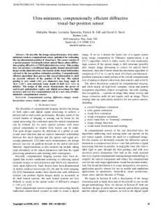
FIG. 1. The raw data produced by (top left) WRF forecast and (top right) stage-IV analysis valid at 0000 UTC 2 Jul 2001 with a 12-h forecast lead time. The resulting binary object images defined by the convolution threshold technique of Davis et al. (2006a) for the (bottom left) WRF forecast and (bottom right) stage IV analysis shown in the top panels. Colors in the bottom panels correspond to merged and matched objects as determined by the method described in the text; gray represents unmatched objects.

image, as well as the best object matches between images. Once the best mergings and matchings have been found, the next step is to compare the two images.

3. Baddeley metric for comparing binary images Our proposed method for merging objects within each image and matching the objects across images makes repeated use of the Baddeley delta metric (Baddeley 1992a,b). Therefore, we summarize this metric here, beginning with a brief discussion of metrics and distances [see Baddeley (1992b) for more on metrics and, in particular, the Hausdorff metric discussed below]. A metric, ⌬, between two sets of pixels A and B contained in a pixel raster X satisfies the following axioms: ⌬共A, B兲 ⫽ 0

⌬ with ␳ and A, B with x, y in Eq. (1). In the present context, the sets of pixels A and B represent objects as defined in section 2. Next, let d(x, A) denote the shortest distance from pixel x ∈ X to the set of pixels, A ⊆ X. That is, d共x, A兲 ⫽ d␳共x, A兲 ⫽ inf{␳共x, a兲 : a ∈ A},

共2兲

with d(x, ⭋) ⬅ ⬁ and ␳(· , ·) a metric.1 Because images can be relatively large, it is important to consider methods that can be rapidly computed; the distance transform algorithm (Borgefors 1986; Rosenfeld and Pfalz 1966, 1968) is useful for computing pixel distances rapidly, and is used in the analyses here. One method for comparing binary images is the

if and only if A ⫽ B;

⌬共A, B兲 ⫽ ⌬共B, A兲 共symmetry兲; ⌬共A, B兲 ⱕ ⌬共A, C兲 ⫹ ⌬共C, B兲 共triangle inequality兲. 共1兲 Similarly, a metric between two pixels x and y, say ␳(x, y), in a raster of pixels can be defined by replacing

1

The inf in Eq. (2) stands for infimum, which is defined as the greatest lower bound of the set. Similarly, for the supremum (sup) of Eq. (3), which is the least upper bound of the set. For sets that contain the greatest lower bound (least upper bound), the infimum (supremum) is equivalent to the minimum (maximum) element of the set.

1750

MONTHLY WEATHER REVIEW

Hausdorff metric, which motivates the Baddeley metric; among others (e.g., Venugopal et al. 2005).

H␳共A, B兲 ⫽

再

A ⫽ ⭋,

andⲐor

B⫽⭋

0,

A⫽⭋

and

B⫽⭋

H␳共A, B兲 ⫽ supx∈X | d共x, A兲 ⫺ d共x, B兲 | .

共4兲

Note that this second definition for H involves pixels from the entire raster, X, instead of simply those in A and B as in the first representation. There are some important problems with Eq. (4). In particular, H has a high sensitivity to noise because a single error pixel can cause elevation of H to its maximum possible value because of the supremum in its definition. See Baddeley (1992a,b) for more on the drawbacks of the Hausdorff metric as an error measure for images. The Baddeley delta metric replaces the supremum in (4) with an Lp norm to stabilize the measure, and a further transformation on d(x, ·) to ensure that the result is a metric. Specifically,

再

Let A, B ⊆ X, with X as a raster of pixels. The Hausdorff distance is given by

max兵supx∈Ad共x, B兲, supx∈Bd共x, A兲其,

with d(x, ·) as defined in Eq. (2). That is, H␳(A, B) is the maximum distance from a point in one set to the nearest point in the other set. Because the sets A and B considered here are finite binary sets, Eq. (3) can be written as

⌬pw共A, B兲 ⫽

VOLUME 136

兺

1 | w关d共x, A兲兴 ⫺ w关d共x, B兲兴 | p N x∈X

冎

1Ⲑp

, 共5兲

where N is the total number of pixels in the raster, X; p is chosen a priori; and w is a concave continuous function that is strictly increasing at zero. For applications, Baddeley (1992a) suggests using the cutoff transformation: w共z兲 ⫽ min{z, c},

共6兲

for a fixed c ⬎ 0. For p → ⬁ in (5), ⌬ tends toward the maximum difference in distances between two sets, and subsequently would be equivalent to (4). For p → 0, ⌬ tends toward the minimum; p ⫽ 1 is the usual arithmetic average for the differences in distance, and p ⫽ 2 gives the average of the common Euclidean norm for each difference [see, e.g., Nychka and Saltzman (1998) or Johnson et al. (1990) for more on Lp norms]. A wide range of choices for p and c will work, and for our purposes, we shall use p ⫽ 2 for computational convenience and efficiency. Note that ⌬pw(A, A) ⫽ ⌬pw(⭋, ⭋) ⫽ 0, and unlike the Hausdorff metric ⌬pw(A, ⭋) ⫽ ⌬pw(⭋, A) ⬍ ⬁.

,

共3兲

Qualitatively, Eq. (5) gives an average of the difference in position of two sets A and B to each point x ∈ X. We show next that with ␻(·) as defined in Eq. (6) and p ⫽ 2, that the metric in (5) is a type of average cluster distance. Three principal cases can be identified within the metric in (5) for two binary image objects A and B, and a given pixel x ∈ X pertaining to the difference w[d(x, 〈)] ⫺ w[d(x, 〉)] when ␻(·) is defined by (6). Namely, (i) d(x, 〈) ⱕ c and d(x, 〉) ⱕ c, (ii) only one of d(x, 〈) and d(x, 〉) is less than or equal to c, or (iii) d(x, 〈) ⬎ c and d(x, 〉) ⬎ c. Using the law of cosines on the first case, it is easy to see that for p ⫽ 2 the squared difference {w[d(x, 〈)] ⫺ w[d(x, 〉)]}2 can be written as

␳2共xA, xB兲 ⫺ 2d共x, A兲d共x, B兲共1 ⫺ cos␪兲,

共7兲

where ␳(xA, xB) is the distance between the point {xA: xA ∈ A and x ∈ X, ␳(xA, x) ⫽ d(x, 〈)} and the point {xB: xB ∈ B and x ∈ X, ␳(xB, x) ⫽ d(x, 〉)}, and ␪ is the angle between the line segments adjoining the point x ∈ X and the two points xA and xB, respectively (Fig. 2). For the second case, the contributions and reductions to the overall metric are relative to a constant term, c, and a (smaller) value relating to the distance between the object nearer to x ∈ X. For the third case, there is no contribution or reduction to the metric because all of the values are zero. Therefore, it can be seen from the form in (7) that ⌬ of Eq. (5) with p ⫽ 2 yields a type of average pixel distance between sets (objects) A and B.

4. Merging and matching binary image objects After initially identifying objects within the analysis and forecast images as in Fig. 1 (bottom row), it is necessary to find the optimal mergings within each image, as well as which objects to match from one image to the other. Ideally, the Baddeley metric (henceforth, ⌬) would be computed for all possible mergings, and each merging compared to each object of the other image. However, if there are m forecast objects and n analysis objects, then there are 2m ⫻ 2n comparisons to make; which would generally be too computationally intensive to be compared operationally. In this section, we propose a method for finding a reasonable subset of the possible mergings.

MAY 2008

GILLELAND ET AL.

FIG. 2. Diagram describing the details behind ⌬ for the case where w(z) ⫽ min{z, c} (c ⬎ 0 constant), p ⫽ 2, d(x, A) ⱕ c, and d(x, B) ⱕ c at a fixed pixel x ∈ X.

The proposed technique computes ⌬ between each of the original objects from one image to the other, and then merges objects in each image based on a ranking of the initial ⌬s. Specifically, let i ⫽ 1, . . . , m denote the ith forecast object, and j ⫽ 1, . . . , n the jth analysis object. 1) Compute ⌬ for each object from the forecast image with each object from the analysis image. For convenience, these ⌬ values are stored in an m ⫻ n matrix, ϒ. 2) Rank the values from step 1. For the ith forecast object, let jk, k ⫽ 1, . . . , n denote the objects with the lowest to highest ⌬ between forecast object i and each analysis object jk. Similarly, for the jth analysis object denote iᐉ, ᐉ ⫽ 1, . . . , m as the objects with the lowest to highest ⌬ when comparing analysis object j to each forecast object iᐉ. 3) Compute ⌬ between the ith forecast object and analysis object j1, then between i and j1 merged together with j2 (i.e., j1 ∪ j2), then i and j1 ∪ j2 ∪ j3, and so on until object i is compared to the merging of all n objects from the analysis image. For convenience, these values are stored in an m ⫻ n matrix, ⌿. 4) Perform step 3 in the other direction. That is, compute ⌬ between object j and i1, j and i1 merged with i2, etc. Again, for convenience, we store these values in an m ⫻ n matrix, ⌶. 5) Merge and match objects by comparing the resulting ⌬ values in the matrices: ϒ, ⌿, and ⌶. Optionally, a threshold, u, may be employed to not allow objects to be matched when ⌬ ⬎ u. This final step is described more explicitly in the text that follows. For step 5 of the above algorithm, let Q ⫽ {ϒ, ⌿, ⌶}. Merge and match objects by comparing the resulting ⌬ values in Q in the following manner. First, those objects

1751

that lead to the smallest ⌬ value in Q are merged and matched together to form the first group of matching objects. To prevent the same object from being matched more than once, the ⌬ values that were computed with any of this first group of objects are removed from Q. Then the smallest ⌬ value is located from those remaining ⌬ values in Q. Objects that give rise to this second smallest ⌬ value are merged and matched to form the second group. This process continues in a similar manner until all objects are exhausted. Note that the above algorithm will allow merged objects from one field to match with single objects from the other field, but will not allow for merged objects in one field to match merged objects in the other field. A further iterative step could be added to allow for such matchings, but at the cost of higher computational burden, and the present study does not explore this possibility.2 The next section will begin with an example of the above algorithm for clarification of the procedure.

5. Results from four test cases Here, the strategy outlined in the previous section is demonstrated with four test cases. These represent typical scenarios from the 100 test cases inspected in this study to give an impression of the strengths and weaknesses of the approach. Note that there are not many objects in these cases so that one could compare all 2m ⫻ 2n combinations, but cases do exist where there are enough objects to make all comparisons expensive. Furthermore, even when 2m ⫻ 2n is not prohibitively large for any given field, the computational burden can still be large when comparing a large number of fields. The first of the four test cases is graphed in Fig. 1, which shows both the raw data (top row) and the binary images with objects labeled with numbers (bottom row) for each of the WRF forecast (left column) and stageIV analysis (right column) as defined by the convolution threshold technique of Brown et al. (2007) and Davis et al. (2006a); this is the same test case as shown in the example of Fig. 2 in Davis et al. (2006a). The binary images for the other three cases are shown in Fig. 3. As mentioned in section 3, a wide range of choices 2 Note that the examples shown in this study do not contain more than eight objects per field so that all 2m ⫻ 2n combinations could be compared, and a more complicated procedure could be employed to allow merged objects from one field to match to merged objects in the other field. This is beyond the scope of this paper as we are interested in an automatic and computationally efficient method that could be used for larger m and n.

1752

MONTHLY WEATHER REVIEW

VOLUME 136

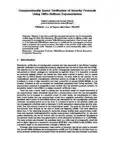
FIG. 3. (left) Binary images for WRF test cases and (right) the corresponding binary images derived from the stage-IV analysis. (top to bottom) Test cases 2–4 corresponding to 0300 and 0900 UTC 2 Jul 2001 (3- and 9-h lead time, respectively), and 0300 UTC 3 Jul 2001 (15-h lead time). Colors correspond to merged and matched objects as determined by the method described in the text; gray represents unmatched objects.

for p and c will work. We use p ⫽ 2 in Eq. (5) for each of these test cases for computational convenience and efficiency. From subjective exploration, we choose c ⫽ 100 pixels, corresponding to about 400 km, as this value consistently yielded reasonable results. Furthermore, we standardize ⌬ to be in the interval [0, 1] by dividing by c. For illustration of the merging and matching procedure detailed in the previous section, we step through

the algorithm for the first test case. Table 1 gives the matrix ϒ from step 1. Note that although the number of objects in each of these fields are the same, this is not necessary for the procedure (the number of objects in either field is arbitrary). Step 2 requires that these values be ranked, and subsequent analyses are based on mergings that progress through these rankings in order to lessen the computational burden in a reasonable manner. The best matches of each forecast object com-

MAY 2008

1753

GILLELAND ET AL.

TABLE 1. Test case 1: values of ⌬ as given by Eq. (5) for 1:1 comparisons of single objects from Fig. 1 (bottom); rows correspond to forecast objects and columns to analysis objects. The best forecast to observation matches (i.e., the smallest value of each row) are in boldface, and the best analysis to forecast matches (i.e., the smallest value of each column) are indicated by *. The best overall match is indicated by **. This is the matrix, ϒ, from step 1 of the algorithm defined in section 4. Analysis objects

Forecast objects

1

2

3

4

5

6

7

8

1 2 3 4 5 6 7 8

0.088* 0.154 0.424 0.327 0.423 0.377 0.474 0.408

0.213 0.177 0.415 0.145* 0.443 0.266 0.455 0.337

0.423 0.395 0.016*,** 0.326 0.076 0.343 0.306 0.377

0.463 0.439 0.123 0.388 0.061* 0.386 0.284 0.404

0.397 0.323 0.404 0.243 0.407 0.108 0.336 0.080*

0.465 0.419 0.294 0.313 0.273 0.230 0.092* 0.215

0.450 0.420 0.334 0.394 0.289 0.320 0.138* 0.292

0.448 0.420 0.350 0.402 0.307 0.324 0.159* 0.293

pared with each analysis object are shown in boldface, and the best match of each analysis object compared to each forecast object are indicated by a superscripted asterisk. Table 2 shows the matrix, ⌿, from step 3 of the algorithm, and Table 3 shows the matrix, ⌶, from step 4. Note that the best overall match from Table 1 matches object 3 from the forecast image to object 3 from the analysis image (⌬ ⬇ 0.02). Because ⌬ does not decrease with any of the mergings (Tables 2 and 3), neither of these objects are merged to any other object. Subjective inspection of Fig. 1 (bottom row) suggests that this result is reasonable as both objects are of roughly the same size, shape, and location. The next best match of single objects matches forecast object 5 with analysis object 4. Again, no better values are obtained by merging objects in the analysis image (see Table 2, row 5), nor are any better values found from merging objects in the forecast image (see Table 3, column 4). Therefore, forecast object 5 is

matched to analysis object 4 without any mergings. Examination of Fig. 1 (bottom row) shows that both objects are small, with forecast object 5 the smaller. There also appears to be a slight spatial (or possibly temporal) displacement where the forecast object lies a little too far to the east as compared with the analysis object 4. Nevertheless, both objects are relatively small in size and similar in location, where forecast object 5 is smaller than analysis object 4 to make comparison of their shapes implausible. Following to the next best single object match, we would compare forecast object 5 to analysis object 3, but as forecast object 5 has already been matched to analysis object 4 with a better ⌬ value (cf. ⬇0.08 and ⬇0.06), and no further mergings improve this value, this matching is not accepted by the procedure. Although the two objects are in the same general area, it is clear that the former match is superior to the latter, indicating that the procedure made a correct decision here. The next best match is between forecast object 8

TABLE 2. Test case 1: values of ⌬ as given by Eq. (5) for single objects from the forecast image compared with merged objects from the analysis image (i.e., the matrix, ⌿, from step 3 of the merging and matching algorithm from section 4). Rows correspond to forecast objects (Fig. 1, bottom left), first column is the best match with single analysis objects (Fig. 1, bottom right), and succeeding columns correspond to mergings between the best and second-best single matches (column 2), the top three matches (column 3), and so on until the last column, which represents the merging of all analysis objects compared with each of the individual forecast objects. Best (smallest) ⌬ values for each row are shown in boldface. Analysis object mergings

Forecast objects

j1

j1 ∪ j2

j1 ∪ j2 ∪ j3

j1 · · · ∪ j4

j1 · · · ∪ j5

j1 · · · ∪ j6

j1 · · · ∪ j7

j1 · · · ∪ j8

1 2 3 4 5 6 7 8

0.088 0.154 0.016 0.145 0.061 0.108 0.092 0.080

0.213 0.185 0.086 0.203 0.090 0.199 0.065 0.186

0.322 0.290 0.226 0.267 0.235 0.314 0.067 0.214

0.421 0.397 0.249 0.315 0.254 0.333 0.200 0.220

0.472 0.453 0.255 0.323 0.260 0.338 0.234 0.369

0.476 0.471 0.358 0.355 0.371 0.398 0.319 0.432

0.502 0.473 0.464 0.372 0.451 0.407 0.449 0.459

0.518 0.498 0.471 0.376 0.495 0.434 0.457 0.467

1754

MONTHLY WEATHER REVIEW

VOLUME 136

TABLE 3. Test case 1: values of ⌬ as given by Eq. (5) for single objects from the analysis image compared with merged objects from the forecast image (i.e., the matrix, ⌶, from step 4 of the merging and matching algorithm from section 4). Rows correspond to forecast objects (Fig. 1), first row is the best match with single forecast objects, and the succeeding rows correspond to mergings between the best and second-best single matches (row 2), the top three matches (row 3), and so on until the last row, which represents the merging of all forecast objects compared with each of the individual analysis objects. Best (smallest) ⌬ values for each column are shown in boldface. Analysis objects

Forecast object mergings

1

2

3

4

5

6

7

8

i1 i 1 ∪ i2 i 1 ∪ i2 ∪ i3 i 1 ∪ · · · ∪ i4 i 1 ∪ · · · ∪ i5 i 1 ∪ · · · ∪ i6 i 1 ∪ · · · ∪ i7 i 1 ∪ · · · ∪ i8

0.088 0.139 0.304 0.347 0.381 0.457 0.473 0.529

0.145 0.098 0.077 0.117 0.162 0.272 0.287 0.359

0.016 0.037 0.230 0.339 0.361 0.383 0.409 0.446

0.061 0.106 0.229 0.323 0.382 0.403 0.429 0.467

00.080 0.088 0.203 0.241 0.339 0.383 0.442 0.447

0.092 0.153 0.186 0.244 0.274 0.335 0.366 0.410

0.138 0.252 0.331 0.360 0.388 0.444 0.468 0.504

0.159 0.267 0.344 0.372 0.401 0.456 0.479 0.514

and analysis object 5, and no further mergings improve the ⌬ value, so this matching is accepted without any mergings. The forecast object here is displaced spatially to the west from this analysis object, and is also a bit smaller. Subjective judgment would likely make this match over the other possibility of matching forecast object 8 with analysis object 6, indicating that the choice based on the procedure is reasonable. One might subjectively match forecast object 6 with analysis object 5, or possibly merge forecast objects 6 and 8 and subsequently match them to the analysis object 5. Nevertheless, the selection by the procedure to match the single forecast object 8 with the single analysis object 5 is consistent with the choice a subjective observer might make. Object 1 from each image shows the next best match. However, careful inspection of matrices ⌿ and ⌶ (Tables 2 and 3, respectively) shows that analysis object 2, when matched with the merging of forecast objects 1, 2, and 4 yields a lower ⌬ than is obtained when simply matching forecast object 1 with analysis object 1. Again, from a subjective point of view, this is a reasonable choice, though the inclusion of analysis object 1 might be desirable (i.e., the merging of analysis objects 1 and 2). This demonstrates a limitation of the approach that merged objects from one field cannot be matched to merged objects from the other field. Nevertheless, the result is reasonable in that a subjective observer could argue against such a merging; analysts might have quite varied interpretations. Objects 7 from the forecast and 6 from the analysis yield the next best single object match from the matrix, ϒ (Table 1). Note that the second best match for forecast object 7 is with analysis object 7. In fact, when these two analysis objects are merged, the match with forecast object 7 provides a much lower ⌬ than the

unmerged case. As there are no better mergings or matchings for these objects, the analysis objects 6 and 7 are merged and together are matched with forecast object 7. Again, this appears reasonable from a subjective standpoint as the forecast object covers much of central Texas beginning on the eastern border with Mexico and ending shortly before the border with Louisiana. Although the analysis objects do not cover much of central Texas, there are no other analysis objects in this area, and there appear to be (spatial) overlaps with these objects and forecast object 7. This may indicate an error in forecast intensity, and one could investigate this by obtaining binary images from the convolution threshold algorithm using different thresholds. Finally, analysis object 8 is in the vicinity of forecast object 7, but is clearly displaced spatially. Inspection of the original raw field (Fig. 1, top row) indicates that the forecast may have indeed overforecast the precipitation intensity over central Texas, and that analysis object 8 appears to be part of the same weather system as objects 6 and 7. This result highlights the important point that this procedure does not account for information in the raw field. Ideally, meteorological information should be used to inform the merging process as important information about the forecast can still be lost in this type of verification scheme, such as spatial displacement, intensity, etc. Table 4 summarizes the results discussed above for the first test case. The ⌬ values for each of these matches are displayed in the last column. Note that analysis objects 1 and 8 are not merged with any other objects, nor are they matched to any objects in the forecast image. As discussed, a subjective observer looking only at the binary object images may or may not merge these objects with other nearby objects. Inspection of the raw fields, however, suggests that both

MAY 2008

TABLE 4. Final results for test case 1. Numbers correspond to object numbers as seen in Fig. 1 (bottom row). Forecast 3 5 7 1, 2, 4 8

Observations

⌬

3 4 6, 7 2 5

0.016 0.061 0.065 0.077 0.080

Unmatched objects 6

1, 8

of these objects are likely part of weather systems that contain these objects so that perhaps the objects should be merged in these cases. Table 5 shows the final results for the second test case (Fig. 3, top row). The procedure merges objects 1, 2, and 4 of the analysis image and matches this to object 2 of the forecast image. This is found to be the best match for this test case. Note that the ⌬ value for this match is relatively higher than those for test case 1 (⌬ ⬇ 0.12 relative to ⌬ ∈ [0.02, 0.08] for test case 1). Indeed, from subjective inspection of 100 test cases from 2 July 2001 to 10 July 2001, a reasonable threshold for ⌬ appears to be about 0.10. Clearly, analysis objects 1 and 2 are heavily displaced to the north of forecast object 2, though there is some overlap. It is not clear from the binary analysis image, or from its corresponding raw field (not shown), that analysis object 4 is part of the same weather system as objects 1 and 2. Nevertheless, the forecast object covers a large region with the southern and northern edges touching all of these analysis objects. Therefore, from a purely binary object viewpoint, the merging and matching is reasonable. Finally, objects 3 from both images are matched with ⌬ ⬇ 0.29. Although the two objects are of about the same size and shape, and at about the same latitude, they are relatively far apart in the east–west direction. Note that ⌬ alone does not indicate whether two objects are different in size or location, but incorporates both criteria into the total. Furthermore, a threshold of 0.30 was used initially on the 100 cases, but inspection of these TABLE 5. Final results for test case 2. Numbers correspond to object numbers as seen in Fig. 3 (top row). Results here are for a threshold of 0.30. Note that there are no matches for the threshold of 0.10, which is found to be a good choice in this study. Forecast 2 3

Observations

⌬

1, 2, 4 3

0.123 0.290

TABLE 6. Final results for test case 3. Numbers correspond to object numbers as seen in Fig. 3 (middle row). Forecast 1

—

Observations

⌬

1

0.029

Unmatched objects 2, 3

—

results suggests that a better threshold would be 0.10 for these data. If this threshold is enforced, then there would be no matches for this case. Final results for test case 3 (Fig. 3, middle row) are given in Table 6. There is only one analysis object for this test case, and it is matched to the unmerged forecast object 1. The two objects overlap spatially, and although both are small, the analysis object is considerably smaller. Finally, Table 7 gives results for test case 4 (Fig. 3, bottom row). This test case is similar to the previous case in that there are not many objects, and the objects are all relatively small in size. Subjectively, one would likely match forecast object 1 with analysis object 2 as these are relatively close in size, shape, and location, although the forecast object is slightly displaced to the east, and covers slightly more area than the corresponding analysis object. One would also likely match forecast object 2 with analysis object 3. Again, the two objects are similar in size, shape, and location, with the forecast object displaced slightly to the south and west from the corresponding analysis object. The small analysis object 1 would likely not be matched to either of the forecast objects as it is spatially very far away from both. The results from applying the merging and matching scheme of section 4 agree with the above subjective arguments. Note also that both ⌬ values are near to 0.10, which, as mentioned above, was generally found to be indicative of poorer agreement between the two objects for all of the 100 test cases. Values larger than this number tend to represent greater discrepancies between images, and values that approach this number tend to be associated with images that are very similar, but show relatively serious departures from each other. TABLE 7. Final results for test case 4. Numbers correspond to object numbers as seen in Fig. 3 (bottom row). Forecast 1 2

Unmatched objects 1

1755

GILLELAND ET AL.

Observations

⌬

2 3

0.065 0.079

Unmatched objects —

1

1756

MONTHLY WEATHER REVIEW

6. Summary and discussion Many methods have been proposed for providing more useful verification of high-resolution spatial forecasts. One class of methods involves the identification of features or objects in each of the forecast and observed fields. For many of these methods it is necessary to somehow identify which, if any, objects within a field should be considered to belong to a larger group of objects within a field (merging). Furthermore, it is often necessary to identify which objects (or groups of objects) should be compared across fields (matching). An automatic and computationally efficient strategy for merging and matching is presented here that is shown to make reasonable merges and matches. The strategy makes heavy use of the Baddeley image metric, ⌬, which is found to be a particularly useful summary metric that accounts for spatial location, coverage, and shape differences among identified features. The Baddeley metric (⌬) provides a useful summary measure for comparing two sets of binary images because it is robust to small changes in location (displacement), orientation, amplitude, and distortion. This is an important feature for verifying forecasts where areas of precipitation may be slightly displaced in time (and subsequently space), but are otherwise relatively accurate. These characteristics are verified by the test cases investigated here. The measure does not, however, distinguish the type of errors that may exist. For example, the metric cannot discern if the differences in the images result from amplitude or distortion errors. For this, one would need to apply other techniques (e.g., Davis et al. 2006a,b; Brown et al. 2007; Ebert and McBride 2000; Hoffman et al. 1995; Micheas et al. 2007; Marzban and Sandgathe 2008). For determining which objects to merge in one image, and which to match between images, the four test cases suggest our approach has great promise, as confirmed by subjective evaluation of 100 test cases. However, the method detailed here relies on using both the forecast and analysis images together in order to determine the best possible mergings. This is acceptable if it is desired to compare only one forecast to the analysis field, but frequently it is desired to compare multiple forecasts using a single reference forecast, such as the analysis field. In such a case, it is generally best to make comparisons using the same analysis image (i.e., with the same object mergings) for all forecast images. Nevertheless, even with this objective in mind, this approach uses the same basic objects in the analysis image to compare against each forecast image. The images only differ in how the individual objects are merged, and in each case they are merged to minimize ⌬ so that

VOLUME 136

one merging does not bias results toward a particular forecast. This is appropriate here because while the merged objects are found to be consistent with how a subjective evaluator might merge objects, they are not merged based on meteorological criterion. It would be useful to allow meteorological covariates (e.g., rainfall regime, storm organization, etc.) to inform the mergings and matchings. Although it may be possible to incorporate such information into the distance metric d(x, A) (e.g., Marzban and Sandgathe 2006, 2008), such a scheme may nullify the computationally efficient distance transform method, making our procedure highly inefficient. Nevertheless, the procedure proposed here allows for a computationally efficient automated method for distinguishing between objects that are close or far apart from one field to another. As a result, the procedure may contribute to other approaches where an algorithm is needed to merge and match binary image objects. Acknowledgments. The authors thank the reviewers for their helpful and constructive comments that made this a better paper. We also thank Cindy Halley Gotway for her assistance with some of the figures. REFERENCES Baddeley, A. J., 1992a: Errors in binary images and an Lp version of the Hausdorff metric. Nieuw Arch. Wiskunde, 10, 157–183. ——, 1992b: An error metric for binary images. Robust Computer Vision: Quality of Vision Algorithms, W. Förstner and S. Ruwiedel, Eds., Wichmann, 59–78. Borgefors, G., 1986: Distance transformations in digital images. Comput. Vision Graphics Image Process., 34 (3), 344–371. Briggs, W. M., and R. A. Levine, 1997: Wavelets and field forecast verification. Mon. Wea. Rev., 125, 1329–1341. Brown, B. G., R. G. Bullock, J. Halley Gotway, D. Ahijevych, E. Gilleland, and L. Holland, 2007: Application of the MODE object-based verification tool for the evaluation of model precipitation fields. Preprints, 22nd Conf. on Weather Analysis and Forecasting/18th Conf. on Numerical Weather Prediction, Park City, UT, Amer. Meteor. Soc., 10A.2. [Available online at http://ams.confex.com/ams/pdfpapers/124856.pdf.] Browning, K. A., C. G. Collier, P. R. Larke, P. Menmuir, G. A. Monk, and R. G. Owens, 1982: On the forecasting of frontal rain using a weather radar network. Mon. Wea. Rev., 110, 534–552. Casati, B., G. Ross, and D. B. Stephenson, 2004: A new intensityscale approach for the verification of spatial precipitation forecasts. Meteor. Appl., 11, 141–154. Davis, C. A., B. G. Brown, and R. G. Bullock, 2006a: Objectbased verification of precipitation forecasts. Part I: Methodology and application to mesoscale rain areas. Mon. Wea. Rev., 134, 1772–1784. ——, ——, and ——, 2006b: Object-based verification of precipitation forecasts. Part II: Application to convective rain systems. Mon. Wea. Rev., 134, 1785–1795. Du, J., and S. L. Mullen, 2000: Removal of distortion error from an ensemble forecast. Mon. Wea. Rev., 128, 3347–3351.

MAY 2008

GILLELAND ET AL.

Ebert, E. E., 2007: Fuzzy verification of high resolution gridded forecasts: A review and proposed framework. Meteor. Appl., in press. ——, and J. L. McBride, 2000: Verification of precipitation in weather systems: Determination of systematic errors. J. Hydrol., 239, 179–202. ——, U. Damrath, W. Wergen, and M. E. Baldwin, 2003: The WGNE assessment of short-term quantitative precipitation forecasts. Bull. Amer. Meteor. Soc., 84, 481–492. Harris, D., E. Foufoula-Georgiou, K. K. Droegemeier, and J. J. Levit, 2001: Multiscale statistical properties of a highresolution precipitation forecast. J. Hydrometeor., 2, 406–418. Hoffman, R. N., Z. Liu, J.-F. Louis, and C. Grassotti, 1995: Distortion representation of forecast errors. Mon. Wea. Rev., 123, 2758–2770. Johnson, M. E., L. M. Moore, and D. Ylvisaker, 1990: Minimax and maximin distance designs. J. Stat. Plann. Inference, 5 (26), 131–148. Lin, Y., and K. E. Mitchell, 2005: The NCEP Stage II/IV hourly precipitation analyses: Development and applications. Preprints, 19th Conf on Hydrology, San Diego, CA, Amer. Meteor. Soc., 1.2 [Available online at http://ams.confex.com/ ams/Annual2005/techprogram/paper_83847.htm.] Marzban, C., and S. Sandgathe, 2006: Cluster analysis for verification of precipitation fields. Wea. Forecasting, 21, 824–838.

1757

——, and ——, 2008: Cluster analysis for object-oriented verification of fields: A variation. Mon. Wea. Rev., 136, 1013–1025. Micheas, A. C., N. I. Fox, S. A. Lack, and C. K. Wikle, 2007: Cell identification and verification of QPF ensembles using shape analysis techniques. J. Hydrol., 343, 105–116. Nychka, D., and N. Saltzman, 1998: Design of air quality monitoring networks. Lecture Notes in Statistics: Case Studies in Environmental Statistics, D. Nychka, W. Piegorsch, and L. Cox, Eds., Springer, 51–76. Rosenfeld, A., and J. L. Pfalz, 1966: Sequential operations in digital picture processing. J. Assoc. Comput. Machinery, 13 (4), 471–494. ——, and ——, 1968: Distance functions on digital pictures. Pattern Recognit., 5, 33–61. Skamarock, W. C., J. B. Klemp, J. Dudhia, D. O. Gill, D. M. Barker, W. Wang, and J. G. Powers, 2005: A description of the advanced research WRF version 2. NCAR Tech. Note NCAR/TN-468⫹STR, 100 pp. [Available online at http:// www.mmm.ucar.edu/wrf/users/docs/arw_v2.pdf.] Venugopal, V., S. Basu, and E. Foufoula-Georgiou, 2005: A new metric for comparing precipitation patterns with an application to ensemble forecasts. J. Geophys. Res., 110, D08111, doi:10.1029/2004JD005395. Wicker, L. J., and W. C. Skamarock, 2002: Time splitting methods for elastic models using forward time schemes. Mon. Wea. Rev., 130, 2088–2097.