OCTOBER 2009
EBERT AND GALLUS
1401
Toward Better Understanding of the Contiguous Rain Area (CRA) Method for Spatial Forecast Verification ELIZABETH E. EBERT Centre for Australian Weather and Climate Research, Melbourne, Victoria, Australia
WILLIAM A. GALLUS JR. Department of Geological and Atmospheric Science, Iowa State University, Ames, Iowa (Manuscript received 17 December 2008, in final form 25 March 2009) ABSTRACT The contiguous rain area (CRA) method for spatial forecast verification is a features-based approach that evaluates the properties of forecast rain systems, namely, their location, size, intensity, and finescale pattern. It is one of many recently developed spatial verification approaches that are being evaluated as part of a Spatial Forecast Verification Methods Intercomparison Project. To better understand the strengths and weaknesses of the CRA method, it has been tested here on a set of idealized geometric and perturbed forecasts with known errors, as well as nine precipitation forecasts from three high-resolution numerical weather prediction models. The CRA method was able to identify the known errors for the geometric forecasts, but only after a modification was introduced to allow nonoverlapping forecast and observed features to be matched. For the perturbed cases in which a radar rain field was spatially translated and amplified to simulate forecast errors, the CRA method also reproduced the known errors except when a high-intensity threshold was used to define the CRA ($10 mm h21) and a large translation error was imposed (.200 km). The decomposition of total error into displacement, volume, and pattern components reflected the source of the error almost all of the time when a mean squared error formulation was used, but not necessarily when a correlation-based formulation was used. When applied to real forecasts, the CRA method gave similar results when either best-fit criteria, minimization of the mean squared error, or maximization of the correlation coefficient, was chosen for matching forecast and observed features. The diagnosed displacement error was somewhat sensitive to the choice of search distance. Of the many diagnostics produced by this method, the errors in the mean and peak rain rate between the forecast and observed features showed the best correspondence with subjective evaluations of the forecasts, while the spatial correlation coefficient (after matching) did not reflect the subjective judgments.
1. Introduction As the spatial and temporal resolution of forecasts from numerical weather prediction (NWP) models grows increasingly finer, there is a need for spatial verification approaches that adequately reflect the quality of these forecasts without overpenalizing errors at the grid scale. Many new spatial verification strategies have been proposed, including neighborhood or fuzzy verification, scale
Corresponding author address: Elizabeth E. Ebert, Bureau of Meteorology Research Centre, GPO Box 1289, Melbourne, VIC 3001 Australia. E-mail:
[email protected] DOI: 10.1175/2009WAF2222252.1 Ó 2009 American Meteorological Society
decomposition, features-based verification, and field deformation approaches [for reviews of these methods, see Casati et al. (2008) and Gilleland et al. (2009)]. These strategies focus on different aspects of forecast quality such as scale-dependent accuracy, location errors, intensity errors, and the realism of the spatial pattern. The majority of these spatial methods require forecasts and observations matched on a common grid. To help users choose the most appropriate verification method(s) for their applications, the Spatial Forecast Verification Methods Intercomparison Project (abbreviated ICP) was begun in 2006 to assess the capabilities, strengths, and weaknesses of the new spatial verification methods (Gilleland et al. 2009; information online at
1402
WEATHER AND FORECASTING
http://www.ral.ucar.edu/projects/icp/index.html). ICP participants evaluated several idealized high-resolution precipitation forecasts with known errors, as well as a set of actual NWP forecasts that had been subjectively evaluated, to see how well the verification methods described the nature of the errors. This paper explores the characteristics of the contiguous rain area (CRA) method, which is one of the early features-based methods (Ebert and McBride 2000). Features-based methods (sometimes called objectoriented or entity-based methods) compare the properties of matched forecast and observed features, where a ‘‘feature’’ is any weather event that can be drawn as a closed contour on a map. Examples of features are rain areas, cloud systems, low pressure centers, and wind maxima. Instead of traditional gridbox-to-gridbox verification, features-based methods verify the location, size, shape, intensity, and other attributes of the feature, and are therefore very intuitive in their interpretation. Other features-based verification methods include the eventsoriented technique of Baldwin and Lakshmivarahan (2003), Nachamkin’s (2004) composite method, the method for object-based diagnostic evaluation (MODE; Davis et al. 2006, 2009), hierarchical cluster analysis (Marzban and Sandgathe 2006, 2008), Procrustes shape analysis (Michaes et al. 2007; Lack et al. 2009), and the structure–amplitude–location (SAL) method of Wernli et al. (2008). One drawback of features-based approaches is that matching is not easily automated. When applied to highresolution rainfall forecasting in the real world, matches are often ambiguous. Two people looking at a pair of rain maps may focus on different aspects of the forecast (e.g., broad scale versus high-intensity cores) and make quite different judgments about what constitutes a feature and what constitutes a good match. Incorrect or inappropriate matches may be made by the automated algorithm, and will lead to the wrong conclusions about forecast quality. A goal of this investigation is therefore to investigate the quality of the matches. When a good match is achieved, what can be learned about the forecast error? When the match is judged imperfect, how does this impact the interpretation of the errors? Section 2 gives an overview of the CRA method. The next three sections investigate the ability of the CRA method to diagnose errors in three sets of continentalscale rainfall forecasts of increasing complexity: idealized geometric forecasts, perturbed ‘‘forecasts’’ to which known errors were applied, and NWP forecasts from three configurations of the Weather Research and Forecasting (WRF) model. The paper concludes with recommendations on the best use of the CRA method.
VOLUME 24
FIG. 1. CRA formed by the overlap of the forecast (ellipse outlined by dashed line, with original position at lower right and final best-fit position at upper left) and the observations (darker ellipse). The stippling shows the CRA before translation of the forecast to the northwest. The heavy black outline shows the region for which verification statistics are computed.
2. CRA verification method The CRA method was developed to evaluate systematic errors in the prediction of rain systems (Ebert and McBride 2000; Grams et al. 2006). It was one of the first methods to measure errors in the predicted location of rain systems and to separate the total error into components due to incorrect location, incorrect amplitude, and differences in finescale pattern. The steps in the CRA technique are described below, which will allow us to interpret the verification results within the context of the algorithm’s methodology. Figure 1 shows the steps schematically. The first step is to look for distinct features or entities that can be associated in the forecast and observation fields. The two fields are assumed to be on the same
OCTOBER 2009
1403
EBERT AND GALLUS
spatial grid. They are merged by overlaying the forecast on the observations and taking the maximum value at each grid point. In this way forecast and observed entities that overlap with each other are now ‘‘associated’’ in the merged field. In other words, the entities are not identified separately in the forecast field and the observed field, but rather in the combined field, which ensures that overlapping forecast and observed entities are matched to each other. An entity finder is next applied to isolate distinct CRAs in the merged field according to some minimum intensity threshold. For hourly rainfall, a typical threshold might be 1 mm h21, but this can be set by the user. Each CRA is assigned a unique identifier (ID). A rectangular bounding box is fit to the CRA and then expanded by a certain distance on all sides to define a search area for the best forecast match. For the ICP idealized cases, the search distance was set to 58 latitude–longitude or the maximum dimension of the CRA, whichever was smaller. For the WRF forecasts examined in the ICP, the search distance was set to 240 km, the value used in Grams et al. (2006) in their study of central U.S. mesoscale convective systems, and the sensitivity to a range of different search distances was tested. Forecast rain features outside the search area are considered to be unrelated to the observed feature. To match the forecast and observed entities within a CRA, the forecast is horizontally translated over the observations until a best-fit criterion is satisfied. The best-fit criterion can be the minimum squared error (Ebert and McBride 2000), maximum correlation coefficient (Grams et al. 2006), or maximum overlap (Ebert et al. 2004). Recent experience in the International H2O Project and elsewhere suggests that the correlation matching is more successful than the minimum squared error matching (Grams et al. 2006; Tartaglione et al. 2005). Both approaches were tested here. The vector defined by the optimal translation gives the estimated location error of the forecast. Finally, the mean squared error (MSE) of the original forecast is decomposed into the displacement (location), volume, and pattern error components; that is, MSEtotal 5 MSEdisplacement 1 MSEvolume 1 MSEpattern . (1) The details of the decomposition have been formulated in two ways, depending on the matching criterion. The original decomposition, used with the minimum squared error best-fit criterion, computes the location component as the difference in the mean squared error before and after shifting the forecast, the volume error as the bias in mean intensity, and the pattern error as a residual:
MSEdisplacement 5 MSEtotal MSEvolume 5 (F
MSEshifted ,
X)2 ,
MSEpattern 5 MSEshifted
(2)
and MSEvolume ,
where F and X are the mean forecast and observed values after the shift. The alternate error decomposition is based on correlation optimization and starts with Murphy’s (1995) decomposition of the MSE: MSEtotal 5 (F
X)2 1 (sX
rsF )2 1 (1
r2 )s2F ,
(3)
where F and X are the mean forecast and observed values before the shift; sF and sX are the standard deviations of the forecast and observed values, respectively; and r is the original spatial correlation between the forecast and observed features. Correcting the forecast location improves its correlation with the observations, ropt. Adding and subtracting ropt and rearranging, MSEdisplacement 5 2sF sX (ropt MSEvolume 5 (F9
r),
X9)2 ,
MSEpattern 5 2sF sX (1
(4)
and
ropt ) 1 (sF
sX )2 .
The expression in Eq. (4) for MSEvolume differs slightly from the corresponding term in the original decomposition [Eq. (2)] as the mean values (denoted F9 and X9) are taken before, rather than after, the shift. In practice this makes little difference. The alternate formulation was developed because occasionally the translation with the greatest correlation led to a value of MSEshifted that was greater than MSEtotal, giving a negative displacement error component in Eq. (2). The pattern errors are computed quite differently in the two error decompositions: in the first formulation [Eq. (2)] as a residual after displacement and volume error have been accounted for, and explicitly in the second decomposition [Eq. (4)] where the terms involving correlation and variability indicate that pattern differences are being measured. Note that spatial shifting of the forecast field during pattern matching can change the size of the CRA by introducing new grid data that were not in the original (misaligned) CRA. The error decomposition is computed from data enclosed within the CRA boundaries before or after the shift. The use of the same set of grid boxes is necessary to make a fair comparison of the errors before and after shifting the forecast. In the example in Fig. 1, any values that were originally to the southeast of the light entity would be ‘‘brought into’’
1404
WEATHER AND FORECASTING
VOLUME 24
TABLE 1. Description of idealized geometric forecasts, and the location error (grid points) and error components (%) for the original and modified CRA verifications. Case
Forecast description
Original CRA results
geom001
Ellipse same as observed but shifted 50 grid points to the east
No match
geom002
Ellipse same as observed but shifted 200 grid points to the east Ellipse similar to observed but centered 125 grid points to the east and horizontally stretched to size 200 3 200
No match
geom004
Ellipse similar to observed but centered 125 grid points to the east and size changed to 200 3 50 (wrong aspect ratio)
No match
geom005
Ellipse similar to observed but centered 125 grid points to the east and horizontally stretched to size 400 3 200
Location error 5 142 points east Location 5 12% Volume 5 47% Pattern 5 41%
geom003
No match
the CRA by the shifting. If these introduced forecast grid boxes contain no rain, then there is no impact, but if they have nonzero values, then the shifting can introduce some apparent error in the error decomposition. An example of this effect is shown in section 4.
3. Results for idealized geometric forecasts The first test was to verify five cases of idealized geometric rain fields. The goal was to establish whether the verification method could return the known errors. As described by Ahijevych et al. (2009, hereafter AGBE), the idealized observed field in each case was a north–south-oriented ellipse of dimension 50 3 200 grid points and of intensity 12.7 mm h21, in which is embedded a higher intensity (25.4 mm h21) ellipse of dimension 20 3 80 points located 10 points to the east of the center (see AGBE’s Fig. 1). The forecasts were similar ellipses, but with their location, size, and aspect ratio altered. Table 1 describes the five idealized forecasts and their corresponding CRA verification results using a threshold of 1 mm h21 to define the entities. The ideal result for an idealized shifting-only experiment is a perfect match. For the CRA verification method this means that the root-mean-square (RMS) error after shifting is exactly 0, the correlation coefficient is exactly 1, and the error decomposition assigns 100% to the displacement component. The diagnosed displacement error did not depend on whether the minimum squared error or the maximum correlation matching criterion was used. When the original CRA method was applied, only one of the five
Modified CRA results Location error 5 50 points east Location 5 100% Volume 5 0% Pattern 5 0% No match Location error 5 142 points east Location 5 44% Volume 5 22% Pattern 5 34% Location error 5 142 points east Location 5 37% Volume 5 0% Pattern 5 63% Location error 5 142 points east Location 5 12% Volume 5 47% Pattern 5 41%
forecasts was successfully matched to the observations, namely geom005. To explain why the CRA method did not achieve matches for any of the other forecasts, it is necessary to look closely at the method. As discussed in section 2, when the forecast and observed entities overlap, then the method tries to match them. However, if the forecast entity is close to the observed entity but not quite touching, there will be two CRAs: one containing the forecast entity but not the observed one, and the other containing the observed entity but not the forecast one (this situation is known as the ‘‘double penalty’’). Because each CRA has a different ID, the method will not attempt to match the observed and forecast entities, even when the forecast entity is within the search area. This is a significant weakness of the method. To address the issue of nearby (but not touching) entities, a simple modification was made to the method so that matching was allowed between forecast and observed entities with different IDs. Matching was achieved in all cases except geom002, where the separation distance between the forecast and observed rain systems was too great. A perfect match was achieved for geom001, as should be the case if the method works correctly. For all cases with distorted forecasts (geom003, geom004, and geom005), the CRA method diagnosed a displacement error of 142 grid points, which represents a mathematically optimal match between the large and small ellipses in the forecasts and observations. This raises the question of what the best match should be when the observed and forecast features look different. Some human analysts would intuitively align the broad
OCTOBER 2009
EBERT AND GALLUS
TABLE 2. Description of idealized perturbed forecasts. Case
Forecast description
pert001
Field shifted 12 km to the east, 20 km to the south Field shifted 24 km to the east, 40 km to the south Field shifted 48 km to the east, 80 km to the south Field shifted 96 km to the east, 160 km to the south Field shifted 192 km to the east, 240 km to the south Field shifted 48 km to the east, 80 km to the south, multiplied by 1.5 Field shifted 48 km to the east, 80 km to the south, 1.27 mm subtracted
pert002 pert003 pert004 pert005 pert006 pert007
lighter rain areas (location error of 125 grid points) while others might match the heavy rain centers (location error of 165–205 grid points). The automated match is between the two. The error decomposition, which reflects the relative contributions of different types of error, agrees with our expectations for these idealized cases. Location was the only source of error for geom001. All error sources were important for geom003, while the geom004 case with an
1405
incorrect aspect ratio showed pattern error to be dominant. Volume error was most important for the geom005 case of strong overprediction. In summary, the CRA verification method correctly diagnosed the nature of the forecast errors for the idealized geometric rain fields, but only when it had been modified to allow matching of two unconnected entities in the forecast and observation fields.
4. Results for idealized perturbed cases While the geometric cases were useful for gaining a basic understanding of the CRA verification method, they do not resemble real rain patterns. The next step in understanding the strengths and weaknesses of the methodology was to test it using realistic-looking forecasts with known errors. These were created by perturbing a model analysis of hourly rainfall to create artificial forecasts, then verifying these forecasts against the original model field. Table 2 lists seven idealized perturbed forecasts created from the WRF model rain forecast shown in Fig. 2. As before, the goal was to establish how well the verification method could return the known errors. In these experiments, five intensity thresholds (1, 2, 5, 10, and 20 mm h21) were used to define CRAs, focusing the verification on rain intensities varying from light to
FIG. 2. WRF model 24-h forecast of hourly rain ending at 0000 UTC 1 Jun 2005, used in perturbed verification experiments. Three broad rain features were manually identified: NGP, SGP, and SE. Smaller objects were identified by CRA verification at higher rain thresholds.
1406
WEATHER AND FORECASTING
VOLUME 24
FIG. 3. CRA verification results for the pert002 case using a CRA threshold of 2 mm h21. The heavy contour shows the isohyet defining the CRA, and the arrow shows the optimal translation of the forecast.
heavy. For each threshold the four largest CRAs (in terms of rain volume) were verified using both the minimum squared error and correlation matching criteria. The unmodified CRA algorithm was used; that is, only overlapping forecast and observed features were treated as CRAs. The forecast displacements determined by the two matching strategies were essentially identical and, in most cases, perfectly diagnosed. For small thresholds and small
to medium displacements there was enough overlap in the two western rain features [northern Great Plains (NGP) and southern Great Plains (SGP) in Fig. 2] that they were treated as a single object. An example is shown in Fig. 3, in which the CRA method perfectly matched the forecast with the observations. As the threshold increased to higher values, the NGP and SGP objects were no longer connected, but matching was still effective (Fig. 4).
OCTOBER 2009
EBERT AND GALLUS
1407
FIG. 4. CRA verification results for the pert003 case using a threshold of 10 mm h21.
Figure 5 summarizes the matching performance of the CRA verification as a function of the detection threshold. Matches were not achieved all of the time. They tended to occur most frequently for lighter rain thresholds and, as expected, for the larger CRAs whose sizes were much greater than the size of the shift. Of 140 CRAs verified (4 CRAs per case 3 7 cases 3 5 thresholds), entities defined by the lower thresholds were matched most of the time. Bull’s-eyes greater than 20 mm h21 proved difficult to match, mainly because of their small sizes. Only two blatantly incorrect matches were made, both of them for the pert004 case that had a rather large imposed displacement. Most of the features in pert005, with a displacement of about 370 km, were not matched at all, which is not surprising since the search region extends only as far as the size of the CRA (up to 58 latitude–longitude). This is not a fault of the verification method, but rather a safeguard to prevent the matching of unrelated features in the forecasts and observations.
When the error decompositions were compared for the two matching methods, the results were somewhat surprising. Sixty-three out of 100 CRAs with prescribed displacements only (cases pert001–pert005) were perfectly matched using both matching strategies, yet many of these did not produce error decompositions with 100% of the error attributed to displacement. This is because new rain pixels were introduced when shifting the forecast (refer to section 2), which led to nonzero RMS errors and correlations of less than 1.0 in some cases. For the minimum squared error matching, 56 out of 63 well-matched cases had the correct displacement error component, that is, 100%. Of the seven imperfect cases, five had displacement error components greater than 90%, which might be considered acceptable, while the worst value was 78%. This CRA corresponded to the light rain area in the northern part of the southeastern United States (SE) rain system, and is shown in Fig. 6. It can be seen from the analysis field that translating the forecast introduced new rain pixels with
1408
WEATHER AND FORECASTING
VOLUME 24
rather than two; however, this could be difficult to implement in an automated verification system. For the pert006 and pert007 cases, where the rain magnitude was multiplied by 1.5 or reduced by subtracting 1.27 mm (0.5 in.), the CRA method correctly attributed a fraction of the error to volume error. In the multiplicative case, the volume error fraction increased as higher CRA thresholds were used and CRAs were smaller in size. To summarize the results from the perturbation experiments, the CRA method correctly matched the forecast and observed objects almost all of the time when the CRAs were defined using light rain thresholds (1–2 mm h21) or were separated by small to moderate distances, but struggled to match widely separated objects that were defined by heavier rain thresholds (10–20 mm h21) and were therefore smaller in extent. When a good match was made, the error decomposition based on the original formulation [Eq. (2)] gave more realistic error components than the alternative one [Eq. (4)] based on correlation optimization.
5. Results for WRF model forecasts FIG. 5. CRA feature-matching performance showing (a) the number of CRAs with the displacement error perfectly diagnosed and (b) the number of unmatched CRAs, as a function of the intensity threshold used to diagnose the CRA. Four CRAs were verified for each case.
intensities greater than 2 mm h21, increasing the value of MSEtotal. For the maximum correlation matching, only 36 of the well-matched cases correctly ascribed 100% of the error to displacement. Of the remaining 27 cases, 10 had displacement error components of less than 90%, with one particularly pathological case having virtually no error attributed to displacement. It appears that the correlationbased error decomposition [Eq. (4)], which relies on the difference between the original and optimal pattern correlations of the features, is less stable than the original squared-error decomposition [Eq. (2)] that relies on the difference between the original and final MSEs. The pert004 example in Figs. 7 and 8 shows how the same feature was matched twice, once when it appeared in the analysis and again when it appeared in the forecast. Only one of these verifications had a reasonable error decomposition using the alternative formulation [Eq. (4)]. It is worth noting that for these same CRAs the original error decomposition [Eq. (2)] assigned 100% and 99.9% of the error to displacement, respectively. These CRAs really should be counted as one match
As a final test of the strengths and weaknesses of the CRA method, verification was performed on 24-h forecasts of 60-min accumulated rainfall for nine convective event cases (Table 3) for which 2- or 4-km configurations of the WRF model were run during the 2005 Storm Prediction Center Spring Program (Kain et al. 2008). One of the WRF configurations was a 2-km horizontal grid spacing run of the Advanced Research WRF (WRF-ARW) performed by the Center for the Analysis and Prediction of Storms (CAPS). This run will be referred to as CAPS2 hereafter. One 4-km version of the WRF-ARW was run by the National Center for Atmospheric Research (hereafter NCAR4) with another 4-km version of the Nonhydrostatic Mesoscale Model (WRF-NMM) run by the National Centers for Environmental Prediction (hereafter NCEP4). All of the forecasts, initialized at 0000 UTC, and stage II precipitation observations were remapped using a neighborbudget interpolation that conserves the total liquid volume in the domain (a procedure typically used at NCEP) to a 4-km Lambert conformal grid before application of the CRA method. The model configurations and nine cases are described in more detail in AGBE. A rainfall threshold of 2.5 mm (0.10 in.) was used to define the objects. Grams et al. (2006) discuss several user-defined parameters in the CRA methodology to which the results for mesoscale convective systems might be sensitive. For the nine cases examined in the ICP, sensitivity to four
OCTOBER 2009
EBERT AND GALLUS
1409
FIG. 6. Third CRA for perturbed case pert001, matched using the minimum squared error criterion.
parameters was explored. Figure 9 uses box-and-whisker plots to show the impacts of changes in two parameters, the search distance and the best-fit criterion, on the rainrate errors for all CRAs identified in the nine cases by the three model configurations. For the sample of nine cases, 24 CRAs were found in the NCAR4 output, 26 in the CAPS2 output, and 29 in the NCEP4 output, regardless of the search distance or the best-fit criterion used. These CRAs contained 50%–55% of the area within the model domain experiencing precipitation, and this fraction did not vary by more than 0.5% as the search distance or best-fit criterion were changed (not shown). For the WRF forecasts, the system rain-rate error is relatively insensitive to changes in the search distance from 120 to 240 to 360 km, and in the use of
MSE minimization instead of correlation coefficient maximization to determine the best fit. It was found that errors in peak rain rate and rain volume were also insensitive to changes in these two parameters (not shown). However, displacement errors, the distance between the centroid of the forecasted rain system and the centroid of the observed one, were more sensitive to the userdefined search distance for all three model configurations (Fig. 10), with general increases in the median values and much larger increases in the upper portion of the range typical for each 120-km increase in the search distance. Displacements generally were not as sensitive, though, to the method of determining the best fit. Although median displacement errors for all three models were roughly 100 km, the magnitude of the average phase shift vector
1410
WEATHER AND FORECASTING
VOLUME 24
FIG. 7. Second CRA for case pert004, using a 2 mm h21 threshold.
(not shown) was less than 20 km, implying no strong systematic bias in the location of the forecasted systems relative to the observed ones. In addition, the phase shift vector was relatively insensitive to the search distance and best-fit criterion when averaged over the CRAs present in the nine cases. The third selectable CRA parameter examined was rainfall threshold. It is reasonable to assume that the verification results will be sensitive to the choice of threshold since a small rainfall threshold will result in larger systems being identified as objects than if a heavier threshold were used. Likewise, the number of systems identified will depend on the threshold. To examine the sensitivity to the threshold, the CRA method was applied using a 1-mm threshold instead of 2.5 mm, while using 240 km as the search distance and MSE minimization to determine the best fit. When the lighter threshold was used, the system-average rain rates decreased and rain volumes and displacement errors increased when
averaged over all CRAs, but the average errors changed by less than ;10% (not shown). Tests with a heavier threshold were not performed but the errors would be expected to change more substantially if a much higher threshold was used since CRAs would be substantially smaller and more difficult to predict correctly. Finally, in section 4 it was seen that for the idealized perturbed cases the decomposition of total error into displacement, volume, and pattern components was somewhat sensitive to whether the MSE-based [Eq. (2)] or correlation-based [Eq. (4)] decomposition was used. To see whether this was also true for real data, the CRA results were compared for verification conducted using the MSE minimization and the correlation maximization best-fit criteria. Table 4 shows that for the nine cases the error breakdown was not very sensitive to the choice of matching method and associated error decomposition, consistent with the results in Figs. 9 and 10. Both approaches showed that on average roughly 30% of the
OCTOBER 2009
1411
EBERT AND GALLUS
FIG. 8. Third CRA for case pert004, using a 2 mm h21 threshold. Although this is the same rain system as in Fig. 7, in that figure the band of heavy rain is in the analysis, while in this figure it is in the forecast.
error could be attributed to displacement of the forecast, 20% to volume errors, and 50% to differences in finescale pattern. A sensitivity test using the lighter 1-mm threshold suggests that the error decomposition values may vary as the rainfall threshold is changed, with the relative contribution of the volume error decreasing and the portion due to pattern error increasing at lighter thresholds. We performed a subjective evaluation of the quality of the matches for the WRF forecasts as diagnosed by the CRA verification method using correlationmaximization fitting and a 1 mm h21 rain threshold. While the quality of the matches depends to a large extent on how well the forecast field resembles the observations, the vast majority of the matches (90%) appeared to be reasonable. Most of the poor matches were characterized by values of the RMS error that were greater than the original (unshifted) error, whereas this occurred
only once when the match was reasonable. About half of the poorly matched CRAs using correlation-maximization fitting were matched well when using the MSE minimization criterion. TABLE 3. Cases for which WRF forecasts were verified using the CRA method. All runs were initialized at 0000 UTC, with verification performed during the 23–24-h forecast period. Case
Date
1 2 3 4 5 6 7 8 9
25 Apr 12 May 13 May 17 May 18 May 24 May 31 May 2 Jun 3 Jun
1412
WEATHER AND FORECASTING
VOLUME 24
FIG. 9. Box-and-whisker plots of rain-rate errors (mm) for all CRAs over all nine cases from three different WRF configurations. Bottoms and tops of boxes show the 25th and 75th percentiles of data, respectively, with median indicated using a horizontal line and whiskers covering the range of the data to at most a distance of 1.5 interquartile ranges, with outliers shown using circles. Shaded boxes are for results using the minimization of the MSE to determine the displacement; clear boxes are for results using maximization of the correlation coefficient. Leftmost two bars for each model represent results using 30 grid points as a search radius, middle two use 60 points, and rightmost two use 90 points.
Unlike the geometric and perturbed cases where the errors are known, the true errors are unknown for the WRF forecasts. As discussed earlier, different people might draw different conclusions when determining which of three forecasts best agrees with the observations or for which of the nine cases the models performed best or worst. Nonetheless, it seems reasonable to expect a useful verification technique to provide results that agree with subjective determinations. AGBE describe a subjective evaluation of the WRF forecasts and indicate that a large amount of variability existed in the subjective evaluations of the three models for these nine cases. Because of the large variability in the ratings, they did not compare the performance of the three model configurations, simply stating that no one configuration performed much better than any other. However, they did show the subjective rankings for the nine cases simulated by one WRF configuration, NCEP4. In Fig. 11, we compare several parameters computed by the CRA verification method (e.g., rain rate, volume) to the AGBE subjective scores for each of the nine cases to examine if some objective measures match better with subjective impressions than other objective measures. All parameters shown in Fig. 11 have been
adjusted so that lower values indicate a better forecast. For these results the CRA verification used a 240-km search distance and MSE minimization to determine the best fit. It is apparent from Fig. 11 that no single objective parameter could be used to rank the performance among the cases and match the ranking of the subjective scores exactly. The measures that correspond most closely are rain-rate error and peak rain-rate error. These both show relatively low amounts of error for the three cases (1, 4, and 8) found by the subjective evaluation to be best forecasted, although they do not always show much larger errors for cases receiving much worse rankings in the subjective evaluation (e.g., case 3). Rain volume error and displacement error do not work as well, with trends between cases often not matching the trends in subjective rankings. The measure with the least correspondence to the subjective evaluation was the pattern correlation after the forecast was shifted to account for displacement error. The differences between these objective measures and subjective rankings are likely influenced by the way in which the subjective evaluation was performed. The forecasts and observations were shown side by side for each case and not overlaid. This technique would make
OCTOBER 2009
1413
EBERT AND GALLUS
FIG. 10. As in Fig. 9 but for displacement errors (km).
it difficult to visually evaluate displacement errors and correlation coefficients that reflect grid-scale (4 km) correlations, and more likely that the evaluator would notice differences in shapes, sizes, and intensities within the color-shaded precipitation fields. Several different combinations of these five parameters were investigated as an index that might correlate well with subjective rankings, but no index was found to match the subjective rankings well consistently.
6. Discussion and recommendations The application of the CRA methodology to the idealized geometric and perturbed cases was a tremendously useful exercise, pointing out many strengths and
flaws in the technique. The verification scheme made good matches in almost all cases where it was possible (i.e., whenever the size of the feature was at least as large as the imposed separation). However, the geometric cases demonstrated that the forecast and observed entities must overlap at least a little bit so that they can be associated with each other and consequently matched. Even the tiniest separation was enough to cause the match to fail. This did not appear to be a serious issue for the more realistic forecasts with greater spatial structure. Nevertheless, it is an undesirable property of the CRA method. When the method was relaxed so that nonoverlapping entities within the search domain could be matched, then the method produced the expected perfect match.
TABLE 4. Error components (% of total error) for each WRF configuration, for two object-matching strategies: MSE minimization and correlation maximization. The results are averaged for all CRAs in the nine cases listed in Table 3. Best-fit criterion for object matching WRF configuration
Error component
MSE minimization
Correlation maximization
NCAR4
Displacement Volume Pattern Displacement Volume Pattern Displacement Volume Pattern
31.8 15.5 52.7 35.3 11.3 53.4 32.1 15.9 51.9
27.3 20.3 52.4 28.7 21.4 49.9 19.7 29.6 50.7
CAPS2
NCEP4
1414
WEATHER AND FORECASTING
VOLUME 24
FIG. 11. Comparison of subjective rankings for the nine cases identified in Table 3 adjusted so that 0 is best and 5 would be worst, with several CRA parameters. The CRA parameters include rain-rate error (mm divided by 2.54), peak rain-rate error (mm divided by 25.4), rain volume error (km3 multiplied by 10), displacement errors (km divided by 100), and correlation coefficient (CC) after forecast shift (expressed as 1 2 CC).
This relaxation may not always be a good strategy, especially if there are two or more forecast entities near one observed entity, or visa versa. In trying to find an optimal match, the method may match neither and produce an estimated forecast displacement that is somewhere in between. A better strategy for addressing this failing would be to first smooth the forecast and observed fields by upscaling to a coarser grid. [This is similar in intent to the image smoothing step in the MODE verification method of Davis et al. (2006).] This would not only enable the matching of features that are nearby but not touching, it could be used in a two-step process to speed up the searching and matching process, which can be time consuming for very high-resolution forecasts. We plan to add this improvement to the CRA verification method in the future. The displacement errors and error decompositions diagnosed by the CRA verification method generally agreed with our expectations. However, sometimes the error decomposition did not adequately reflect the true nature of the prescribed errors in the idealized perturbed experiments. The main source of error in the decomposition relates to the introduction of new points into the domain when the forecast is shifted. This normally causes only a small deviation from the correct decomposition, at least using the original formulation [Eq. (2)] in which the displacement error is simply the difference between the MSE before and after the shift. The alternative error decomposition [Eq. (4)], based on
maximum correlation matching, appears to be more susceptible to giving misleading results. The likely cause is the greater sensitivity of the correlation coefficient for the optimal translation, ropt, to the introduced points in the shifted forecast field, as compared to the sensitivity of MSEshifted. Comparisons of error components from the two formulations showed quite good agreement on nine real cases, so there may be less reason to question the decomposition results when the correlation-based formulation is used. Nevertheless, we recommend using the original error decomposition [Eq. (2)] whenever possible (i.e., whenever MSEshifted is less than MSEtotal), no matter which matching criterion is chosen for use in the method. It was found that errors in rain rate, peak rain rate, and rain volume for the nine WRF forecasts were relatively insensitive to two of the tunable parameters of the CRA method, namely search distance and method of determining the best fit with observations. Displacement error was not particularly sensitive to the best-fit method, but was sensitive to the search distance used. The ability of the method to make a good match also depended on the intensity threshold used to define the CRA. The user therefore should select values of these parameters that appropriately reflect the size and intensity of the forecasts to be evaluated (Grams et al. 2006). It should be noted that the cases evaluated here generally have rain located in the center of a large domain. Therefore, they are not susceptible to the ‘‘domain
OCTOBER 2009
1415
EBERT AND GALLUS
jumping’’ behavior observed by Tartaglione et al. (2005) and Grams et al. (2006) whereby the verification scheme minimizes the total squared error by shifting the forecast feature out of the domain. This undesirable behavior does not occur when correlation matching is used. We therefore recommend that for matching forecast and observed features the correlation maximization approach be used in preference to the error minimization approach, especially when verifying features near the domain boundaries. Degradation of the MSE after correlation matching may indicate that a poor match has been made, in which case it may be desirable to recompute the CRA verification using the error minimization approach. We also reiterate Tartaglione et al.’s (2005) recommendation that the CRA verification method be applied only when the forecast and observation domain is significantly larger than the features being evaluated. This ensures that the verification results are representative of complete rain systems and that appropriate matching can be done. A comparison of the CRA results for the nine WRF forecasts with subjective evaluations discussed in AGBE found that the errors in entity-based mean and peak rain rates agreed best with subjective evaluations of forecast performance among cases, but even for these two variables substantial disagreement existed for some cases. The rain volume error, displacement error, and correlation coefficient of the shifted forecast showed much less agreement with the subjective ratings. Further work is necessary to determine if some combination of CRA results might better match or more consistently match subjective impressions. The CRA verification method is designed to evaluate the properties of rain systems or other weather events that can be thought of as objects. The idealized and WRF forecast samples tested in the ICP so far fit this description quite well (AGBE; Gilleland et al. 2009). However, not all rain is as well organized and objectlike as the cases shown here. Future experiments in the ICP will examine cases of large-scale and scattered rain, for which the CRA methodology may not be as well suited. It will be instructive to see what the CRA method has to offer in those cases. Acknowledgments. The authors thank the organizers of the Spatial Forecast Verification Methods Intercomparison Project, namely Eric Gilleland, Dave Ahijevych, Barb Brown, Paul Kucera, and Chris Davis for instigating and coordinating a very useful and enlightening activity. We also thank Nazario Tartaglione and two other anonymous reviewers for their many helpful suggestions.
REFERENCES Ahijevych, D., E. Gilleland, B. Brown, and E. E. Ebert, 2009: Application of spatial verification methods to idealized and NWP gridded precipitation forecasts. Wea. Forecasting, in press. Baldwin, M. E., and S. Lakshmivarahan, 2003: Development of an events-oriented verification system using data mining and image processing algorithms. Preprints, Third Conf. on Artificial Intelligence Applications to Environmental Science, Long Beach, CA, Amer. Meteor. Soc., 4.6. [Available online at http://ams.confex.com/ams/pdfpapers/57821.pdf.] Casati, B., and Coauthors, 2008: Forecast verification: Current status and future directions. Meteor. Appl., 15, 3–18. Davis, C., B. Brown, and R. Bullock, 2006: Object-based verification of precipitation forecasts. Part I: Methods and application to mesoscale rain areas. Mon. Wea. Rev., 134, 1772–1784. ——, ——, ——, and J. Halley-Gotway, 2009: The Method for Object-Based Diagnostic Evaluation (MODE) applied to numerical forecasts from the 2005 NSSL/SPC spring program. Wea. Forecasting, 24, 1252–1267. Ebert, E. E., and J. L. McBride, 2000: Verification of precipitation in weather systems: Determination of systematic errors. J. Hydrol., 239, 179–202. ——, L. J. Wilson, B. G. Brown, P. Nurmi, H. E. Brooks, J. Bally, and M. Jaeneke, 2004: Verification of nowcasts from the WWRP Sydney 2000 Forecast Demonstration Project. Wea. Forecasting, 19, 73–96. Gilleland, E., D. Ahijevych, B. G. Brown, and E. E. Ebert, 2009: Intercomparison of spatial forecast verification methods. Wea. Forecasting, 24, 1416–1430. Grams, J. S., W. A. Gallus, L. S. Wharton, S. Koch, A. Loughe, and E. E. Ebert, 2006: The use of a modified Ebert–McBride technique to evaluate mesoscale model QPF as a function of convective system morphology during IHOP 2002. Wea. Forecasting, 21, 288–306. Kain, J. S., and Coauthors, 2008: Some practical considerations regarding horizontal resolution in the first generation of operational convection-allowing NWP. Wea. Forecasting, 23, 931–952. Lack, S. A., G. L. Limpert, and N. I. Fox, 2009: An object-oriented multiscale verification scheme. Wea. Forecasting, in press. Marzban, C., and S. Sandgathe, 2006: Cluster analysis for verification of precipitation fields. Wea. Forecasting, 21, 824–838. ——, and ——, 2008: Cluster analysis for object-oriented verification of fields: A variation. Mon. Wea. Rev., 136, 1013–1025. Michaes, A. C., N. I. Fox, S. A. Lack, and C. K. Wikle, 2007: Cell identification and verification of QPF ensembles using shape analysis techniques. J. Hydrol., 343, 105–116. Murphy, A. H., 1995: The coefficients of correlation and determination as measures of performance in forecast verification. Wea. Forecasting, 10, 681–688. Nachamkin, J. E., 2004: Mesoscale verification using meteorological composites. Mon. Wea. Rev., 132, 941–955. Tartaglione, N., S. Mariani, C. Accadia, A. Speranza, and M. Casaioli, 2005: Comparison of rain gauge observations with modeled precipitation over Cyprus using contiguous rain area analysis. Atmos. Chem. Phys., 5, 2147–2154. Wernli, H., M. Paulat, M. Hagen, and C. Frei, 2008: SAL—A novel quality measure for the verification of quantitative precipitation forecasts. Mon. Wea. Rev., 136, 4470–4487.