prepared by David Mount for the course CMSC 427, Computer Graphics, ...... of
the locations of light sources, their shape, and the color and directional prop-.
CMSC 427 Computer Graphics1 David M. Mount Department of Computer Science University of Maryland Spring 2004
1 Copyright, David M. Mount, 2004, Dept. of Computer Science, University of Maryland, College Park, MD, 20742. These lecture notes were prepared by David Mount for the course CMSC 427, Computer Graphics, at the University of Maryland. Permission to use, copy, modify, and distribute these notes for educational purposes and without fee is hereby granted, provided that this copyright notice appear in all copies.
Lecture Notes
1
CMSC 427
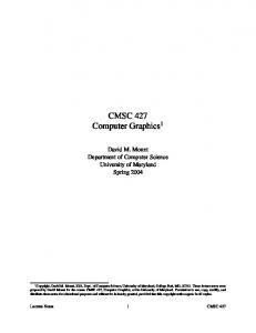
Lecture 1: Course Introduction Reading: Chapter 1 in Hearn and Baker. Computer Graphics: Computer graphics is concerned with producing images and animations (or sequences of images) using a computer. This includes the hardware and software systems used to make these images. The task of producing photo-realistic images is an extremely complex one, but this is a field that is in great demand because of the nearly limitless variety of applications. The field of computer graphics has grown enormously over the past 10–20 years, and many software systems have been developed for generating computer graphics of various sorts. This can include systems for producing 3-dimensional models of the scene to be drawn, the rendering software for drawing the images, and the associated user-interface software and hardware. Our focus in this course will not be on how to use these systems to produce these images (you can take courses in the art department for this), but rather in understanding how these systems are constructed, and the underlying mathematics, physics, algorithms, and data structures needed in the construction of these systems. The field of computer graphics dates back to the early 1960’s with Ivan Sutherland, one of the pioneers of the field. This began with the development of the (by current standards) very simple software for performing the necessary mathematical transformations to produce simple line-drawings of 2- and 3-dimensional scenes. As time went on, and the capacity and speed of computer technology improved, successively greater degrees of realism were achievable. Today it is possible to produce images that are practically indistinguishable from photographic images (or at least that create a pretty convincing illusion of reality). Course Overview: Given the state of current technology, it would be possible to design an entire university major to cover everything (important) that is known about computer graphics. In this introductory course, we will attempt to cover only the merest fundamentals upon which the field is based. Nonetheless, with these fundamentals, you will have a remarkably good insight into how many of the modern video games and “Hollywood” movie animations are produced. This is true since even very sophisticated graphics stem from the same basic elements that simple graphics do. They just involve much more complex light and physical modeling, and more sophisticated rendering techniques. In this course we will deal primarily with the task of producing a single image from a 2- or 3-dimensional scene model. This is really a very limited aspect of computer graphics. For example, it ignores the role of computer graphics in tasks such as visualizing things that cannot be described as such scenes. This includes rendering of technical drawings including engineering charts and architectural blueprints, and also scientific visualization such as mathematical functions, ocean temperatures, wind velocities, and so on. We will also ignore many of the issues in producing animations. We will produce simple animations (by producing lots of single images), but issues that are particular to animation, such as motion blur, morphing and blending, temporal anti-aliasing, will not be covered. They are the topic of a more advanced course in graphics. Let us begin by considering the process of drawing (or rendering) a single image of a 3-dimensional scene. This is crudely illustrated in the figure below. The process begins by producing a mathematical model of the object to be rendered. Such a model should describe not only the shape of the object but its color, its surface finish (shiny, matte, transparent, fuzzy, scaly, rocky). Producing realistic models is extremely complex, but luckily it is not our main concern. We will leave this to the artists and modelers. The scene model should also include information about the location and characteristics of the light sources (their color, brightness), and the atmospheric nature of the medium through which the light travels (is it foggy or clear). In addition we will need to know the location of the viewer. We can think of the viewer as holding a “synthetic camera”, through which the image is to be photographed. We need to know the characteristics of this camera (its focal length, for example). Based on all of this information, we need to perform a number of steps to produce our desired image. Projection: Project the scene from 3-dimensional space onto the 2-dimensional image plane in our synthetic camera.
Lecture Notes
2
CMSC 427
Light sources
Object model Viewer Image plane
Fig. 1: A typical rendering situation. Color and shading: For each point in our image we need to determine its color, which is a function of the object’s surface color, its texture, the relative positions of light sources, and (in more complex illumination models) the indirect reflection of light off of other surfaces in the scene. Hidden surface removal: Elements that are closer to the camera obscure more distant ones. We need to determine which surfaces are visible and which are not. Rasterization: Once we know what colors to draw for each point in the image, the final step is that of mapping these colors onto our display device. By the end of the semester, you should have a basic understanding of how each of the steps is performed. Of course, a detailed understanding of most of the elements that are important to computer graphics will beyond the scope of this one-semester course. But by combining what you have learned here with other resources (from books or the Web) you will know enough to, say, write a simple video game, write a program to generate highly realistic images, or produce a simple animation. The Course in a Nutshell: The process that we have just described involves a number of steps, from modeling to rasterization. The topics that we cover this semester will consider many of these issues. Basics: Graphics Programming: OpenGL, graphics primitives, color, viewing, event-driven I/O, GL toolkit, frame buffers. Geometric Programming: Review of linear algebra, affine geometry, (points, vectors, affine transformations), homogeneous coordinates, change of coordinate systems. Implementation Issues: Rasterization, clipping. Modeling: Model types: Polyhedral models, hierarchical models, fractals and fractal dimension. Curves and Surfaces: Representations of curves and surfaces, interpolation, Bezier, B-spline curves and surfaces, NURBS, subdivision surfaces. Surface finish: Texture-, bump-, and reflection-mapping. Projection: 3-d transformations and perspective: Scaling, rotation, translation, orthogonal and perspective transformations, 3-d clipping. Hidden surface removal: Back-face culling, z-buffer method, depth-sort. Issues in Realism: Light and shading: Diffuse and specular reflection, the Phong and Gouraud shading models, light transport and radiosity.
Lecture Notes
3
CMSC 427
Ray tracing: Ray-tracing model, reflective and transparent objects, shadows. Color: Gamma-correction, halftoning, and color models. Although this order represents a “reasonable” way in which to present the material. We will present the topics in a different order, mostly to suit our need to get material covered before major programming assignments.
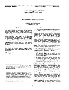
Lecture 2: Graphics Systems and Models Reading: Today’s material is covered roughly in Chapters 2 and 4 of our text. We will discuss the drawing and filling algorithms of Chapter 4, and OpenGL commands later in the semester. Elements of Pictures: Computer graphics is all about producing pictures (realistic or stylistic) by computer. Before discussing how to do this, let us first consider the elements that make up images and the devices that produce them. How are graphical images represented? There are four basic types that make up virtually of computer generated pictures: polylines, filled regions, text, and raster images. Polylines: A polyline (or more properly a polygonal curve is a finite sequence of line segments joined end to end. These line segments are called edges, and the endpoints of the line segments are called vertices. A single line segment is a special case. (An infinite line, which stretches to infinity on both sides, is not usually considered to be a polyline.) A polyline is closed if it ends where it starts. It is simple if it does not self-intersect. Self-intersections include such things as two edge crossing one another, a vertex intersecting in the interior of an edge, or more than two edges sharing a common vertex. A simple, closed polyline is also called a simple polygon. If all its internal angle are at most 180◦ , then it is a convex polygon. A polyline in the plane can be represented simply as a sequence of the (x, y) coordinates of its vertices. This is sufficient to encode the geometry of a polyline. In contrast, the way in which the polyline is rendered is determined by a set of properties call graphical attributes. These include elements such as color, line width, and line style (solid, dotted, dashed), how consecutive segments are joined (rounded, mitered or beveled; see the book for further explanation).
Closed polyline
Simple polyline
No joint
Mitered
Simple polygon Convex polygon
Rounded
Beveled
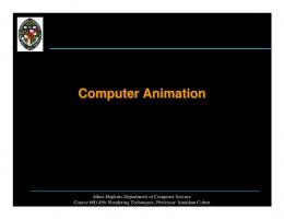
Fig. 2: Polylines and joint styles. Many graphics systems support common special cases of curves such as circles, ellipses, circular arcs, and Bezier and B-splines. We should probably include curves as a generalization of polylines. Most graphics drawing systems implement curves by breaking them up into a large number of very small polylines, so this distinction is not very important. Filled regions: Any simple, closed polyline in the plane defines a region consisting of an inside and outside. (This is a typical example of an utterly obvious fact from topology that is notoriously hard to prove. It is called the Jordan curve theorem.) We can fill any such region with a color or repeating pattern. In some instances the bounding polyline itself is also drawn and others the polyline is not drawn.
Lecture Notes
4
CMSC 427
A polyline with embedded “holes” also naturally defines a region that can be filled. In fact this can be generalized by nesting holes within holes (alternating color with the background color). Even if a polyline is not simple, it is possible to generalize the notion of interior. Given any point, shoot a ray to infinity. If it crosses the boundary an odd number of times it is colored. If it crosses an even number of times, then it is given the background color.
with boundary
without boundary
with holes
self intersecting
Fig. 3: Filled regions. Text: Although we do not normally think of text as a graphical output, it occurs frequently within graphical images such as engineering diagrams. Text can be thought of as a sequence of characters in some font. As with polylines there are numerous attributes which affect how the text appears. This includes the font’s face (Times-Roman, Helvetica, Courier, for example), its weight (normal, bold, light), its style or slant (normal, italic, oblique, for example), its size, which is usually measured in points, a printer’s unit of measure equal to 1/72-inch), and its color.
Face (family)
Weight
Style (slant)
Size
Helvetica
Normal Bold
Normal Italic
8 point
Times−Roman Courier
10 point
12 point Fig. 4: Text font properties.
Raster Images: Raster images are what most of us think of when we think of a computer generated image. Such an image is a 2-dimensional array of square (or generally rectangular) cells called pixels (short for “picture elements”). Such images are sometimes called pixel maps. The simplest example is an image made up of black and white pixels, each represented by a single bit (0 for black and 1 for white). This is called a bitmap. For gray-scale (or monochrome) raster images raster images, each pixel is represented by assigning it a numerical value over some range (e.g., from 0 to 255, ranging from black to white). There are many possible ways of encoding color images. We will discuss these further below. Graphics Devices: The standard interactive graphics device today is called a raster display. As with a television, the display consists of a two-dimensional array of pixels. There are two common types of raster displays. Video displays: consist of a screen with a phosphor coating, that allows each pixel to be illuminated momentarily when struck by an electron beam. A pixel is either illuminated (white) or not (black). The level of intensity can be varied to achieve arbitrary gray values. Because the phosphor only holds its color briefly, the image is repeatedly rescanned, at a rate of at least 30 times per second. Liquid crystal displays (LCD’s): use an electronic field to alter polarization of crystalline molecules in each pixel. The light shining through the pixel is already polarized in some direction. By changing the polarization of the pixel, it is possible to vary the amount of light which shines through, thus controlling its intensity.
Lecture Notes
5
CMSC 427
Irrespective of the display hardware, the computer program stores the image in a two-dimensional array in RAM of pixel values (called a frame buffer). The display hardware produces the image line-by-line (called raster lines). A hardware device called a video controller constantly reads the frame buffer and produces the image on the display. The frame buffer is not a device. It is simply a chunk of RAM memory that has been allocated for this purpose. A program modifies the display by writing into the frame buffer, and thus instantly altering the image that is displayed. An example of this type of configuration is shown below. CPU
I/O Devices
System bus
Memory
Frame Buffer
Video Controller
Monitor
Simple Raster Graphics System CPU
I/O Devices
System bus
System Memory
Display Processor
Frame
Memory
Buffer
Video Controller
Monitor
Raster Graphics with Display Processor
Fig. 5: Raster display architectures. More sophisticated graphics systems, which are becoming increasingly common these days, achieve great speed by providing separate hardware support, in the form of a display processor (more commonly known as a graphics accelerator or graphics card to PC users). This relieves the computer’s main processor from much of the mundane repetitive effort involved in maintaining the frame buffer. A typical display processor will provide assistance for a number of operations including the following: Transformations: Rotations and scalings used for moving objects and the viewer’s location. Clipping: Removing elements that lie outside the viewing window. Projection: Applying the appropriate perspective transformations. Shading and Coloring: The color of a pixel may be altered by increasing its brightness. Simple shading involves smooth blending between some given values. Modern graphics cards support more complex procedural shading. Texturing: Coloring objects by “painting” textures onto their surface. Textures may be generated by images or by procedures. Hidden-surface elimination: Determines which of the various objects that project to the same pixel is closest to the viewer and hence is displayed. An example of this architecture is shown in Fig. 5. These operations are often pipelined, where each processor on the pipeline performs its task and passes the results to the next phase. Given the increasing demands on a top quality graphics accelerator, they have become quite complex. Fig. 6 shows the architecture of existing accelerator. (Don’t worry about understanding the various elements just now.)
Lecture Notes
6
CMSC 427
Graphics port Host bus interface Video I/O interface
Command engine 2−d Engine
3−d Engine
VGA graphics controller Display engine
Transform, clip, lighting
Video Engine
Vertex skinning
DVD/ HDTV decoder
Vertex cache
Hardware cursor
TMDS transmitter
Keyframe interpolation
Scaler
D/A converter Texture units
Pixel cache
Renderer
Texture cache
Graphics stream
Renderer
Digital monitor
Ratiometric expander
Pallette and overlay control
Triangle setup
YUV to RGB
Video input port
Scaler
Analog monitor
YUV/ RGB
Video stream
z−buffer Memory controller and interface
Synchronous DRAM or double data−rate memory
Fig. 6: The architecture of a sample graphics accelerator. Color: The method chosen for representing color depends on the characteristics of the graphics output device (e.g., whether it is additive as are video displays or subtractive as are printers). It also depends on the number of bits per pixel that are provided, called the pixel depth. For example, the most method used currently in video and color LCD displays is a 24-bit RGB representation. Each pixel is represented as a mixture of red, green and blue components, and each of these three colors is represented as a 8-bit quantity (0 for black and 255 for the brightest color). In many graphics systems it is common to add a fourth component, sometimes called alpha, denoted A. This component is used to achieve various special effects, most commonly in describing how opaque a color is. We will discuss its use later in the semester. For now we will ignore it. In some instances 24-bits may be unacceptably large. For example, when downloading images from the web, 24-bits of information for each pixel may be more than what is needed. A common alternative is to used a color map, also called a color look-up-table (LUT). (This is the method used in most gif files, for example.) In a typical instance, each pixel is represented by an 8-bit quantity in the range from 0 to 255. This number is an index to a 256-element array, each of whose entries is a 234-bit RGB value. To represent the image, we store both the LUT and the image itself. The 256 different colors are usually chosen so as to produce the best possible reproduction of the image. For example, if the image is mostly blue and red, the LUT will contain many more blue and red shades than others. A typical photorealistic image contains many more than 256 colors. This can be overcome by a fair amount of clever trickery to fool the eye into seeing many shades of colors where only a small number of distinct colors exist. This process is called digital halftoning, as shown in Fig. 8. Colors are approximated by putting combinations of similar colors in the same area. The human eye averages them out.
Lecture Notes
7
CMSC 427
Colormap R
Frame buffer
G
B
121 122 176 002
123 015 154 247
031 123
124 125
Fig. 7: Color-mapped color.
Fig. 8: Color approximation by digital halftoning. (Note that you are probably not seeing the true image, since has already been halftoned by your document viewer or printer.)
Lecture Notes
8
CMSC 427
Lecture 3: Drawing in OpenGL: GLUT Reading: Chapter 2 in Hearn and Baker. Detailed documentation on GLUT can be downloaded from the GLUT home page http://www.opengl.org/resources/libraries/glut.html. The OpenGL API: Today we will begin discussion of using OpenGL, and its related libraries, GLU (which stands for the OpenGL utility library) and GLUT (an OpenGL Utility Toolkit). OpenGL is designed to be a machineindependent graphics library, but one that can take advantage of the structure of typical hardware accelerators for computer graphics. The Main Program: Before discussing how to actually draw shapes, we will begin with the basic elements of how to create a window. OpenGL was intentionally designed to be independent of any specific window system. Consequently, a number of the basic window operations are not provided. For this reason, a separate library, called GLUT or OpenGL Utility Toolkit, was created to provide these functions. It is the GLUT toolkit which provides the necessary tools for requesting that windows be created and providing interaction with I/O devices. Let us begin by considering a typical main program. Throughout, we will assume that programming is done in C++. Do not worry for now if you do not understand the meanings of the various calls. Later we will discuss the various elements in more detail. This program creates a window that is 400 pixels wide and 300 pixels high, located in the upper left corner of the display. Typical OpenGL/GLUT Main Program // program arguments
int main(int argc, char** argv) { glutInit(&argc, argv);
// initialize glut and gl // double buffering and RGB glutInitDisplayMode(GLUT_DOUBLE | GLUT_RGB); glutInitWindowSize(400, 300); // initial window size glutInitWindowPosition(0, 0); // initial window position glutCreateWindow(argv[0]); // create window ...initialize callbacks here (described below)... myInit(); glutMainLoop(); return 0;
// your own initializations // turn control over to glut // (make the compiler happy)
}
Here is an explanation of the first five function calls. glutInit(): The arguments given to the main program (argc and argv) are the command-line arguments supplied to the
program. This assumes a typical Unix environment, in which the program is invoked from a command line. We pass these into the main initialization procedure, glutInit(). This procedure must be called before any others. It processes (and removes) command-line arguments that may be of interest to GLUT and the window system and does general initialization of GLUT and OpenGL. Any remaining arguments are then left for the user’s program to interpret, if desired. glutInitDisplayMode(): The next procedure, glutInitDisplayMode(), performs initializations informing OpenGL how to
set up its frame buffer. Recall that the frame buffer is a special 2-dimensional array in main memory where the graphical image is stored. OpenGL maintains an enhanced version of the frame buffer with additional information. For example, this include depth information for hidden surface removal. The system needs to know how we are representing colors of our general needs in order to determine the depth (number of bits) to assign for each pixel in the frame buffer. The argument to glutInitDisplayMode() is a logical-or (using the operator “—”) of a number of possible options, which are given in Table 1. Lecture Notes
9
CMSC 427
Display Mode GLUT RGB GLUT RGBA GLUT INDEX GLUT DOUBLE GLUT SINGLE GLUT DEPTH
Meaning Use RGB colors Use RGB plus α (for transparency) Use colormapped colors (not recommended) Use double buffering (recommended) Use single buffering (not recommended) Use depth buffer (needed for hidden surface removal)
Table 1: Arguments to glutInitDisplayMode(). . Color: First off, we need to tell the system how colors will be represented. There are three methods, of which two are fairly commonly used: GLUT RGB or GLUT RGBA. The first uses standard RGB colors (24-bit color, consisting of 8 bits of red, green, and blue), and is the default. The second requests RGBA coloring. In this color system there is a fourth component (A or α), which indicates the opaqueness of the color (1 = fully opaque, 0 = fully transparent). This is useful in creating transparent effects. We will discuss how this is applied later this semester. Single or Double Buffering: The next option specifies whether single or double buffering is to be used, GLUT SINGLE or GLUT DOUBLE, respectively. To explain the difference, we need to understand a bit more about how the frame buffer works. In raster graphics systems, whatever is written to the frame buffer is immediately transferred to the display. (Recall this from Lecture 2.) This process is repeated frequently, say 30–60 times a second. To do this, the typical approach is to first erase the old contents by setting all the pixels to some background color, say black. After this, the new contents are drawn. However, even though it might happen very fast, the process of setting the image to black and then redrawing everything produces a noticeable flicker in the image. Double buffering is a method to eliminate this flicker. In double buffering, the system maintains two separate frame buffers. The front buffer is the one which is displayed, and the back buffer is the other one. Drawing is always done to the back buffer. Then to update the image, the system simply swaps the two buffers. The swapping process is very fast, and appears to happen instantaneously (with no flicker). Double buffering requires twice the buffer space as single buffering, but since memory is relatively cheap these days, it is the preferred method for interactive graphics. Depth Buffer: One other option that we will need later with 3-dimensional graphics will be hidden surface removal. This fastest and easiest (but most space-consuming) way to do this is with a special array called a depth buffer. We will discuss in greater detail later, but intuitively this is a 2-dimensional array which stores the distance (or depth) of each pixel from the viewer. This makes it possible to determine which surfaces are closest, and hence visible, and which are farther, and hence hidden. The depth buffer is enabled with the option GLUT DEPTH. For this program it is not needed, and so has been omitted. glutInitWindowSize(): This command specifies the desired width and height of the graphics window. The general form is glutInitWindowSize(int width, int height). The values are given in numbers of pixels. glutInitPosition(): This command specifies the location of the upper left corner of the graphics window. The form is glutInitWindowPosition(int x, int y) where the (x, y) coordinates are given relative to the upper left
corner of the display. Thus, the arguments (0, 0) places the window in the upper left corner of the display. Note that glutInitWindowSize() and glutInitWindowPosition() are both considered to be only suggestions to the system as to how to where to place the graphics window. Depending on the window system’s policies, and the size of the display, it may not honor these requests. glutCreateWindow(): This command actually creates the graphics window. The general form of the command is glutCreateWindowchar(*title), where title is a character string. Each window has a title, and the argument is a string which specifies the window’s title. We pass in argv[0]. In Unix argv[0] is the name of the program
(the executable file name) so our graphics window’s name is the same as the name of our program. Lecture Notes
10
CMSC 427
Note that glutCreateWindow() does not really create the window, but rather sends a request to the system that the window be created. Thus, it is not possible to start sending output to the window, until notification has been received that this window is finished its creation. This is done by a display event callback, which we describe below. Event-driven Programming and Callbacks: Virtually all interactive graphics programs are event driven. Unlike traditional programs that read from a standard input file, a graphics program must be prepared at any time for input from any number of sources, including the mouse, or keyboard, or other graphics devises such as trackballs and joysticks. In OpenGL this is done through the use of callbacks. The graphics program instructs the system to invoke a particular procedure whenever an event of interest occurs, say, the mouse button is clicked. The graphics program indicates its interest, or registers, for various events. This involves telling the window system which event type you are interested in, and passing it the name of a procedure you have written to handle the event. Types of Callbacks: Callbacks are used for two purposes, user input events and system events. User input events include things such as mouse clicks, the motion of the mouse (without clicking) also called passive motion, keyboard hits. Note that your program is only signaled about events that happen to your window. For example, entering text into another window’s dialogue box will not generate a keyboard event for your program. There are a number of different events that are generated by the system. There is one such special event that every OpenGL program must handle, called a display event. A display event is invoked when the system senses that the contents of the window need to be redisplayed, either because: • the graphics window has completed its initial creation, • an obscuring window has moved away, thus revealing all or part of the graphics window, • the program explicitly requests redrawing, by calling glutPostRedisplay(). Recall from above that the command glutCreateWindow() does not actually create the window, but merely requests that creation be started. In order to inform your program that the creation has completed, the system generates a display event. This is how you know that you can now start drawing into the graphics window. Another type of system event is a reshape event. This happens whenever the window’s size is altered. The callback provides information on the new size of the window. Recall that your initial call to glutInitWindowSize() is only taken as a suggestion of the actual window size. When the system determines the actual size of your window, it generates such a callback to inform you of this size. Typically, the first two events that the system will generate for any newly created window are a reshape event (indicating the size of the new window) followed immediately by a display event (indicating that it is now safe to draw graphics in the window). Often in an interactive graphics program, the user may not be providing any input at all, but it may still be necessary to update the image. For example, in a flight simulator the plane keeps moving forward, even without user input. To do this, the program goes to sleep and requests that it be awakened in order to draw the next image. There are two ways to do this, a timer event and an idle event. An idle event is generated every time the system has nothing better to do. This may generate a huge number of events. A better approach is to request a timer event. In a timer event you request that your program go to sleep for some period of time and that it be “awakened” by an event some time later, say 1/30 of a second later. In glutTimerFunc() the first argument gives the sleep time as an integer in milliseconds and the last argument is an integer identifier, which is passed into the callback function. Various input and system events and their associated callback function prototypes are given in Table 2. For example, the following code fragment shows how to register for the following events: display events, reshape events, mouse clicks, keyboard strikes, and timer events. The functions like myDraw() and myReshape() are supplied by the user, and will be described later. Most of these callback registrations simply pass the name of the desired user function to be called for the corresponding event. The one exception is glutTimeFunc() whose arguments are the number of milliseconds to Lecture Notes
11
CMSC 427
Input Event Mouse button Mouse motion Keyboard key System Event (Re)display (Re)size window Timer event Idle event
User callback function prototype (return void) myMouse(int b, int s, int x, int y) myMotion(int x, int y) myKeyboard(unsigned char c, int x, int y) User callback function prototype (return void) myDisplay() myReshape(int w, int h) myTimer(int id) myIdle()
Callback request glutMouseFunc glutPassiveMotionFunc glutKeyboardFunc Callback request glutDisplayFunc glutReshapeFunc glutTimerFunc glutIdleFunc
Table 2: Common callbacks and the associated registration functions. Typical Callback Setup int main(int argc, char** argv) { ... glutDisplayFunc(myDraw); glutReshapeFunc(myReshape); glutMouseFunc(myMouse); glutKeyboardFunc(myKeyboard); glutTimerFunc(20, myTimeOut, 0); ... }
// set up the callbacks
// (see below)
wait (an unsigned int), the user’s callback function, and an integer identifier. The identifier is useful if there are multiple timer callbacks requested (for different times in the future), so the user can determine which one caused this particular event. Callback Functions: What does a typical callback function do? This depends entirely on the application that you are designing. Some examples of general form of callback functions is shown below. Examples of Callback Functions for System Events void myDraw() { // called to display window // ...insert your drawing code here ... } void myReshape(int w, int h) { // called if reshaped windowWidth = w; // save new window size windowHeight = h; // ...may need to update the projection ... glutPostRedisplay(); // request window redisplay } void myTimeOut(int id) { // called if timer event // ...advance the state of animation incrementally... glutPostRedisplay(); // request redisplay glutTimerFunc(20, myTimeOut, 0); // request next timer event }
Note that the timer callback and the reshape callback both invoke the function glutPostRedisplay(). This procedure informs OpenGL that the state of the scene has changed and should be redrawn (by calling your drawing procedure). This might be requested in other callbacks as well. Note that each callback function is provided with information associated with the event. For example, a reshape Lecture Notes
12
CMSC 427
Examples of Callback Functions for User Input Events // called if mouse click void myMouse(int b, int s, int x, int y) { switch (b) { // b indicates the button case GLUT_LEFT_BUTTON: if (s == GLUT_DOWN) // button pressed // ... else if (s == GLUT_UP) // button released // ... break; // ... // other button events } } // called if keyboard key hit void myKeyboard(unsigned char c, int x, int y) { switch (c) { // c is the key that is hit case ’q’: // ’q’ means quit exit(0); break; // ... // other keyboard events } }
event callback passes in the new window width and height. A mouse click callback passes in four arguments, which button was hit (b: left, middle, right), what the buttons new state is (s: up or down), the (x, y) coordinates of the mouse when it was clicked (in pixels). The various parameters used for b and s are described in Table 3. A keyboard event callback passes in the character that was hit and the current coordinates of the mouse. The timer event callback passes in the integer identifier, of the timer event which caused the callback. Note that each call to glutTimerFunc() creates only one request for a timer event. (That is, you do not get automatic repetition of timer events.) If you want to generate events on a regular basis, then insert a call to glutTimerFunc() from within the callback function to generate the next one. GLUT Parameter Name GLUT LEFT BUTTON GLUT MIDDLE BUTTON GLUT RIGHT BUTTON GLUT DOWN GLUT UP
Meaning left mouse button middle mouse button right mouse button mouse button pressed down mouse button released
Table 3: GLUT parameter names associated with mouse events.
Lecture 4: Drawing in OpenGL: Drawing and Viewports Reading: Chapters 2 and 3 in Hearn and Baker. Basic Drawing: We have shown how to create a window, how to get user input, but we have not discussed how to get graphics to appear in the window. Today we discuss OpenGL’s capabilities for drawing objects. Before being able to draw a scene, OpenGL needs to know the following information: what are the objects to be drawn, how is the image to be projected onto the window, and how lighting and shading are to be performed. Lecture Notes
13
CMSC 427
To begin with, we will consider a very the simple case. There are only 2-dimensional objects, no lighting or shading. Also we will consider only relatively little user interaction. Because we generally do not have complete control over the window size, it is a good idea to think in terms of drawing on a rectangular idealized drawing region, whose size and shape are completely under our control. Then we will scale this region to fit within the actual graphics window on the display. More generally, OpenGL allows for the grahics window to be broken up into smaller rectangular subwindows, called viewports. We will then have OpenGL scale the image drawn in the idealized drawing region to fit within the viewport. The main advantage of this approach is that it is very easy to deal with changes in the window size. We will consider a simple drawing routine for the picture shown in the figure. We assume that our idealized drawing region is a unit square over the real interval [0, 1] × [0, 1]. (Throughout the course we will use the notation [a, b] to denote the interval of real values z such that a ≤ z ≤ b. Hence, [0, 1] × [0, 1] is a unit square whose lower left corner is the origin.) This is illustrated in Fig. 9. 1
red blue
0.5
0 0
0.5
1
Fig. 9: Drawing produced by the simple display function. Glut uses the convention that the origin is in the upper left corner and coordinates are given as integers. This makes sense for Glut, because its principal job is to communicate with the window system, and most window systems (X-windows, for example) use this convention. On the other hand, OpenGL uses the convention that coordinates are (generally) floating point values and the origin is in the lower left corner. Recalling the OpenGL goal is to provide us with an idealized drawing surface, this convention is mathematically more elegant. The Display Callback: Recall that the display callback function is the function that is called whenever it is necessary to redraw the image, which arises for example: • The initial creation of the window, • Whenever the window is uncovered by the removal of some overlapping window, • Whenever your program requests that it be redrawn (through the use of glutPostRedisplay() function, as in the case of an animation, where this would happen continuously. The display callback function for our program is shown below. We first erase the contents of the image window, then do our drawing, and finally swap buffers so that what we have drawn becomes visible. (Recall double buffering from the previous lecture.) This function first draws a red diamond and then (on top of this) it draws a blue rectangle. Let us assume double buffering is being performed, and so the last thing to do is invoke glutSwapBuffers() to make everything visible. Let us present the code, and we will discuss the various elements of the solution in greater detail below. Clearing the Window: The command glClear() clears the window, by overwriting it with the background color. This is set by the call glClearColor(GLfloat Red, GLfloat Green, GLfloat Blue, GLfloat Alpha).
Lecture Notes
14
CMSC 427
Sample Display Function // display function
void myDisplay() { glClear(GL_COLOR_BUFFER_BIT);
// clear the window
glColor3f(1.0, 0.0, 0.0); glBegin(GL_POLYGON); glVertex2f(0.90, 0.50); glVertex2f(0.50, 0.90); glVertex2f(0.10, 0.50); glVertex2f(0.50, 0.10); glEnd();
// set color to red // draw a diamond
glColor3f(0.0, 0.0, 1.0); glRectf(0.25, 0.25, 0.75, 0.75);
// set color to blue // draw a rectangle
glutSwapBuffers();
// swap buffers
}
The type GLfloat is OpenGL’s redefinition of the standard float. To be correct, you should use the approved OpenGL types (e.g. GLfloat, GLdouble, GLint) rather than the obvious counterparts (float, double, and int). Typically the GL types are the same as the corresponding native types, but not always. Colors components are given as floats in the range from 0 to 1, from dark to light. Recall from Lecture 2 that the A (or α) value is used to control transparency. For opaque colors A is set to 1. Thus to set the background color to black, we would use glClearColor(0.0, 0.0, 0.0, 1.0), and to set it to blue use glClearColor(0.0, 0.0, 1.0, 1.0). (Hint: When debugging your program, it is often a good idea to use an uncommon background color, like a random shade of pink, since black can arise as the result of many different bugs.) Since the background color is usually independent of drawing, the function glClearColor() is typically set in one of your initialization procedures, rather than in the drawing callback function. Clearing the window involves resetting information within the frame buffer. As we mentioned before, the frame buffer may store different types of information. This includes color information, of course, but depth or distance information is used for hidden surface removal. Typically when the window is cleared, we want to clear everything, but occasionally it is possible to achieve special effects by erasing only part of the buffer (just the colors or just the depth values). So the glClear() command allows the user to select what is to be cleared. In this case we only have color in the depth buffer, which is selected by the option GL COLOR BUFFER BIT. If we had a depth buffer to be cleared it as well we could do this by combining these using a “bitwise or” operation: glClear(GL COLOR BUFFER BIT — GL DEPTH BUFFER BIT)
Drawing Attributes: The OpenGL drawing commands describe the geometry of the object that you want to draw. More specifically, all OpenGL is based on drawing objects with straight sides, so it suffices to specify the vertices of the object to be drawn. The manner in which the object is displayed is determined by various drawing attributes (color, point size, line width, etc.). The command glColor3f() sets the drawing color. The arguments are three GLfloat’s, giving the R, G, and B components of the color. In this case, RGB = (1, 0, 0) means pure red. Once set, the attribute applies to all subsequently defined objects, until it is set to some other value. Thus, we could set the color, draw three polygons with the color, then change it, and draw five polygons with the new color. This call illustrates a common feature of many OpenGL commands, namely flexibility in argument types. The suffix “3f” means that three floating point arguments (actually GLfloat’s) will be given. For example, glColor3d() takes three double (or GLdouble) arguments, glColor3ui() takes three unsigned int arguments, and so on. For Lecture Notes
15
CMSC 427
floats and doubles, the arguments range from 0 (no intensity) to 1 (full intensity). For integer types (byte, short, int, long) the input is assumed to be in the range from 0 (no intensity) to its maximum possible positive value (full intensity). But that is not all! The three argument versions assume RGB color. If we were using RGBA color instead, we would use glColor4d() variant instead. Here “4” signifies four arguments. (Recall that the A or alpha value is used for various effects, such an transparency. For standard (opaque) color we set A = 1.0.) In some cases it is more convenient to store your colors in an array with three elements. The suffix “v” means that the argument is a vector. For example glColor3dv() expects a single argument, a vector containing three GLdouble’s. (Note that this is a standard C/C++ style array, not the class vector from the C++ Standard Template Library.) Using C’s convention that a vector is represented as a pointer to its first element, the corresponding argument type would be “const GLdouble*”. Whenever you look up the prototypes for OpenGL commands, you often see a long list, some of which are shown below. void glColor3d(GLdouble red, GLdouble green, GLdouble blue) void glColor3f(GLfloat red, GLfloat green, GLfloat blue) void glColor3i(GLint red, GLint green, GLint blue) ... (and forms for byte, short, unsigned byte and unsigned short) ... void glColor4d(GLdouble red, GLdouble green, GLdouble blue, GLdouble alpha) ... (and 4-argument forms for all the other types) ... void glColor3dv(const GLdouble *v) ... (and other 3- and 4-argument forms for all the other types) ...
Drawing commands: OpenGL supports drawing of a number of different types of objects. The simplest is glRectf(), which draws a filled rectangle. All the others are complex objects consisting of a (generally) unpredictable number of elements. This is handled in OpenGL by the constructs glBegin(mode) and glEnd(). Between these two commands a list of vertices is given, which defines the object. The sort of object to be defined is determined by the mode argument of the glBegin() command. Some of the possible modes are illustrated in Fig. 10. For details on the semantics of the drawing methods, see the reference manuals. Note that in the case of GL POLYGON only convex polygons (internal angles less than 180 degrees) are supported. You must subdivide nonconvex polygons into convex pieces, and draw each convex piece separately. glBegin(mode); glVertex(v0); glVertex(v1); ... glEnd();
In the example above we only defined the x- and y-coordinates of the vertices. How does OpenGL know whether our object is 2-dimensional or 3-dimensional? The answer is that it does not know. OpenGL represents all vertices as 3-dimensional coordinates internally. This may seem wasteful, but remember that OpenGL is designed primarily for 3-d graphics. If you do not specify the z-coordinate, then it simply sets the z-coordinate to 0.0. By the way, glRectf() always draws its rectangle on the z = 0 plane. Between any glBegin()...glEnd() pair, there is a restricted set of OpenGL commands that may be given. This includes glVertex() and also other command attribute commands, such as glColor3f(). At first it may seem a bit strange that you can assign different colors to the different vertices of an object, but this is a very useful feature. Depending on the shading model, it allows you to produce shapes whose color blends smoothly from one end to the other. There are a number of drawing attributes other than color. For example, for points it is possible adjust their size (with glPointSize()). For lines, it is possible to adjust their width (with glLineWidth()), and create dashed Lecture Notes
16
CMSC 427
v5
v5
v0 v3 v1
v3 v1
v2
v5 v2 v3 v2
GL TRIANGLES
v5
v0
v1
GL TRIANGLE STRIP
v3 v1
v2
v6
v4 v2
GL TRIANGLE FAN
v2
v3
GL_POLYGON
v6
v6
v4
v0
v2 v3 v 4
v3 v1
v1
GL_LINE_LOOP
v7
v4
v4
v2
v5
v0
v3
v0
v4
GL_LINE_STRIP
v6
v4
v4
v3 v1
v2
v5
v0
v4
GL_LINES
v0
v5
v0
v4
GL_POINTS
v1
v5
v0
v1
v2
GL QUADS
v5
v7 v3 v5
v0
v1
GL QUAD STRIP
Fig. 10: Some OpenGL object definition modes. or dotted lines (with glLineStipple()). It is also possible to pattern or stipple polygons (with glPolygonStipple()). When we discuss 3-dimensional graphics we will discuss many more properties that are used in shading and hidden surface removal. After drawing the diamond, we change the color to blue, and then invoke glRectf() to draw a rectangle. This procedure takes four arguments, the (x, y) coordinates of any two opposite corners of the rectangle, in this case (0.25, 0.25) and (0.75, 0.75). (There are also versions of this command that takes double or int arguments, and vector arguments as well.) We could have drawn the rectangle by drawing a GL POLYGON, but this form is easier to use. Viewports: OpenGL does not assume that you are mapping your graphics to the entire window. Often it is desirable to subdivide the graphics window into a set of smaller subwindows and then draw separate pictures in each window. The subwindow into which the current graphics are being drawn is called a viewport. The viewport is typically the entire display window, but it may generally be any rectangular subregion. The size of the viewport depends on the dimensions of our window. Thus, every time the window is resized (and this includes when the window is created originally) we need to readjust the viewport to ensure proper transformation of the graphics. For example, in the typical case, where the graphics are drawn to the entire window, the reshape callback would contain the following call which resizes the viewport, whenever the window is resized. void myReshape(int winWidth, int winHeight) { ... glViewport (0, 0, winWidth, winHeight); ... }
Setting the Viewport in the Reshape Callback // reshape window
// reset the viewport
The other thing that might typically go in the myReshape() function would be a call to glutPostRedisplay(), since you will need to redraw your image after the window changes size. The general form of the command is glViewport(GLint x, GLint y, GLsizei width, GLsizei height),
Lecture Notes
17
CMSC 427
where (x, y) are the pixel coordinates of the lower-left corner of the viewport, as defined relative to the lower-left corner of the window, and width and height are the width and height of the viewport in pixels. Projection Transformation: In the simple drawing procedure, we said that we were assuming that the “idealized” drawing area was a unit square over the interval [0, 1] with the origin in the lower left corner. The transformation that maps the idealized drawing region (in 2- or 3-dimensions) to the window is called the projection. We did this for convenience, since otherwise we would need to explicitly scale all of our coordinates whenever the user changes the size of the graphics window. However, we need to inform OpenGL of where our “idealized” drawing area is so that OpenGL can map it to our viewport. This mapping is performed by a transformation matrix called the projection matrix, which OpenGL maintains internally. (In the next lecture we will discuss OpenGL’s transformation mechanism in greater detail. In the mean time some of this may seem a bit arcane.) Since matrices are often cumbersome to work with, OpenGL provides a number of relatively simple and natural ways of defining this matrix. For our 2-dimensional example, we will do this by simply informing OpenGL of the rectangular region of two dimensional space that makes up our idealized drawing region. This is handled by the command gluOrtho2D(left, right, bottom, top).
First note that the prefix is “glu” and not “gl”, because this procedure is provided by the GLU library. Also, note that the “2D” designator in this case stands for “2-dimensional.” (In particular, it does not indicate the argument types, as with, say, glColor3f()). All arguments are of type GLdouble. The arguments specify the x-coordinates (left and right) and the ycoordinates (bottom and top) of the rectangle into which we will be drawing. Any drawing that we do outside of this region will automatically be clipped away by OpenGL. The code to set the projection is given below. Setting a Two-Dimensional Projection // set projection matrix // initialize to identity // map unit square to viewport
glMatrixMode(GL_PROJECTION); glLoadIdentity(); gluOrtho2D(0.0, 1.0, 0.0, 1.0);
The first command tells OpenGL that we are modifying the projection transformation. (OpenGL maintains three different types of transformations, as we will see later.) Most of the commands that manipulate these matrices do so by multiplying some matrix times the current matrix. Thus, we initialize the current matrix to the identity, which is done by glLoadIdentity(). This code usually appears in some initialization procedure or possibly in the reshape callback. Where does this code fragment go? It depends on whether the projection will change or not. If we make the simple assumption that are drawing will always be done relative to the [0, 1]2 unit square, then this code can go in some initialization procedure. If our program decides to change the drawing area (for example, growing the drawing area when the window is increased in size) then we would need to repeat the call whenever the projection changes. At first viewports and projections may seem confusing. Remember that the viewport is a rectangle within the actual graphics window on your display, where you graphics will appear. The projection defined by gluOrtho2D() simply defines a rectangle in some “ideal” coordinate system, which you will use to specify the coordinates of your objects. It is the job of OpenGL to map everything that is drawn in your ideal window to the actual viewport on your screen. This is illustrated in Fig. 11. The complete program is shown in Figs. 12 and 13.
Lecture Notes
18
CMSC 427
Drawing
gluOrtho2d
glViewport viewport
top
height bottom left
(x,y) width
right
idealized drawing region
Your graphics window
Fig. 11: Projection and viewport transformations.
#include #include
// standard definitions // C++ I/O
#include #include #include
// GLUT // GLU // OpenGL
using namespace std;
// make std accessible
// ... insert callbacks here int main(int argc, char** argv) { glutInit(&argc, argv); // OpenGL initializations glutInitDisplayMode(GLUT_DOUBLE | GLUT_RGB);// double buffering and RGB glutInitWindowSize(400, 400); // create a 400x400 window glutInitWindowPosition(0, 0); // ...in the upper left glutCreateWindow(argv[0]); // create the window glutDisplayFunc(myDisplay); glutReshapeFunc(myReshape); glutMainLoop(); return 0;
// setup callbacks // start it running // ANSI C expects this
}
Fig. 12: Sample OpenGL Program: Header and Main program.
Lecture Notes
19
CMSC 427
void myReshape(int w, int h) { glViewport (0, 0, w, h); glMatrixMode(GL_PROJECTION); glLoadIdentity(); gluOrtho2D(0.0, 1.0, 0.0, 1.0); glMatrixMode(GL_MODELVIEW); glutPostRedisplay(); }
// window is reshaped // update the viewport // update projection
void myDisplay(void) { glClearColor(0.5, 0.5, 0.5, 1.0); glClear(GL_COLOR_BUFFER_BIT); glColor3f(1.0, 0.0, 0.0); glBegin(GL_POLYGON); glVertex2f(0.90, 0.50); glVertex2f(0.50, 0.90); glVertex2f(0.10, 0.50); glVertex2f(0.50, 0.10); glEnd(); glColor3f(0.0, 0.0, 1.0); glRectf(0.25, 0.25, 0.75, 0.75); glutSwapBuffers(); }
// // // // //
// map unit square to viewport // request redisplay
(re)display callback background is gray clear the window set color to red draw the diamond
// set color to blue // draw the rectangle // swap buffers
Fig. 13: Sample OpenGL Program: Callbacks.
Lecture 5: Drawing in OpenGL: Transformations Reading: Transformation are discussed (for 3-space) in Chapter 5. Two dimensional projections and the viewport transformation are discussed at the start of Chapter 6. For reference documentation, visit the OpenGL documentation links on the course web page. More about Drawing: So far we have discussed how to draw simple 2-dimensional objects using OpenGL. Suppose that we want to draw more complex scenes. For example, we want to draw objects that move and rotate or to change the projection. We could do this by computing (ourselves) the coordinates of the transformed vertices. However, this would be inconvenient for us. It would also be inefficient, since we would need to retransmit all the vertices of these objects to the display processor with each redrawing cycle, making it impossible for the display processor to cache recently processed vertices. For this reason, OpenGL provides tools to handle transformations. Today we consider how this is done in 2-space. This will form a foundation for the more complex transformations, which will be needed for 3-dimensional viewing. Transformations: Linear and affine transformations are central to computer graphics. Recall from your linear algebra class that a linear transformation is a mapping in a vector space that preserves linear combinations. Such transformations include rotations, scalings, shearings (which stretch rectangles into parallelograms), and combinations thereof. Affine transformations are somewhat more general, and include translations. We will discuss affine transformations in detail in a later lecture. The important features of both transformations is that they map straight lines to straight lines, they preserve parallelism, and they can be implemented through matrix multiplication. They arise in various ways in graphics. Moving Objects: from frame to frame in an animation. Change of Coordinates: which is used when objects that are stored relative to one reference frame are to be accessed in a different reference frame. One important case of this is that of mapping objects stored in a standard coordinate system to a coordinate system that is associated with the camera (or viewer). Lecture Notes
20
CMSC 427
Projection: is used to project objects from the idealized drawing window to the viewport, and mapping the viewport to the graphics display window. (We shall see that perspective projection transformations are more general than affine transformations, since they may not preserve parallelism.) Mapping: between surfaces, for example, transformations that indicate how textures are to be wrapped around objects, as part of texture mapping. OpenGL has a very particular model for how transformations are performed. Recall that when drawing, it was convenient for us to first define the drawing attributes (such as color) and then draw a number of objects using that attribute. OpenGL uses much the same model with transformations. You specify a transformation, and then this transformation is automatically applied to every object that is drawn, until the transformation is set again. It is important to keep this in mind, because it implies that you must always set the transformation prior to issuing drawing commands. Because transformations are used for different purposes, OpenGL maintains three sets of matrices for performing various transformation operations. These are: Modelview matrix: Used for transforming objects in the scene and for changing the coordinates into a form that is easier for OpenGL to deal with. (It is used for the first two tasks above). Projection matrix: Handles parallel and perspective projections. (Used for the third task above.) Texture matrix: This is used in specifying how textures are mapped onto objects. (Used for the last task above.) We will discuss the texture matrix later in the semester, when we talk about texture mapping. There is one more transformation that is not handled by these matrices. This is the transformation that maps the viewport to the display. It is set by glViewport(). Understanding how OpenGL maintains and manipulates transformations through these matrices is central to understanding how OpenGL works. This is not merely a “design consideration,” since most display processors maintain such a set of matrices in hardware. For each matrix type, OpenGL maintains a stack of matrices. The current matrix is the one on the top of the stack. It is the matrix that is being applied at any given time. The stack mechanism allows you to save the current matrix (by pushing the stack down) and restoring it later (by popping the stack). We will discuss the entire process of implementing affine and projection transformations later in the semester. For now, we’ll give just basic information on OpenGL’s approach to handling matrices and transformations. OpenGL has a number of commands for handling matrices. In order to know which matrix (Modelview, Projection, or Texture) to which an operation applies, you can set the current matrix mode. This is done with the following command glMatrixMode(hmodei);
where hmodei is either GL MODELVIEW, GL PROJECTION, or GL TEXTURE. The default mode is GL MODELVIEW. GL MODELVIEW is by far the most common mode, the convention in OpenGL programs is to assume that you are always in this mode. If you want to modify the mode for some reason, you first change the mode to the desired mode (GL PROJECTION or GL TEXTURE), perform whatever operations you want, and then immediately change the mode back to GL MODELVIEW.
Once the matrix mode is set, you can perform various operations to the stack. OpenGL has an unintuitive way of handling the stack. Note that most operations below (except glPushMatrix()) alter the contents of the matrix at the top of the stack. glLoadIdentity(): Sets the current matrix to the identity matrix. glLoadMatrix*(M): Loads (copies) a given matrix over the current matrix. (The ‘*’ can be either ‘f’ or ‘d’ depending on whether the elements of M are GLfloat or GLdouble, respectively.)
Lecture Notes
21
CMSC 427
glMultMatrix*(M): Multiplies the current matrix by a given matrix and replaces the current matrix with this result. (As above, the ‘*’ can be either ‘f’ or ‘d’ depending on M .) glPushMatrix(): Pushes a copy of the current matrix on top the stack. (Thus the stack now has two copies of the
top matrix.) glPopMatrix(): Pops the current matrix off the stack.
We will discuss how matrices like M are presented to OpenGL later in the semester. There are a number of other matrix operations, which we will also discuss later.
C
I
M
CM
C C
B A
B A
B A
B A
B A
B A
initial stack
load identity
push matrix
pop matrix
load mult matrix(M) matrix(M)
Fig. 14: Matrix stack operations. Automatic Evaluation and the Transformation Pipeline: Now that we have described the matrix stack, the next question is how do we apply the matrix to some point that we want to transform? Understanding the answer is critical to understanding how OpenGL (and actually display processors) work. The answer is that it happens automatically. In particular, every vertex (and hence virtually every geometric object that is drawn) is passed through a series of matrices, as shown in Fig. 15. This may seem rather inflexible, but it is because of the simple uniformity of sending every vertex through this transformation sequence that makes graphics cards run so fast. Indeed, this is As mentioned above, these transformations behave much like drawing attributes—you set them, do some drawing, alter them, do more drawing, etc. Perspective Point (from glVertex)
Modelview
Projection
normalization
Viewport
Matrix
Matrix
and clipping
Transformation
Standard
Camera (or eye)
coordinates
coordinates
Normalized device coordinates
Window coordinates
Fig. 15: Transformation pipeline. A second important thing to understand is that OpenGL’s transformations do not alter the state of the objects you are drawing. They simply modify things before they get drawn. For example, suppose that you draw a unit square (U = [0, 1] × [0, 1]) and pass it through a matrix that scales it by a factor of 5. The square U itself has not changed; it is still a unit square. If you wanted to change the actual representation of U to be a 5 × 5 square, then you need to perform your own modification of U ’s representation. You might ask, “what if I do not want the current transformation to be applied to some object?” The answer is, “tough luck.” There are no exceptions to this rule (other than commands that act directly on the viewport). If you do not want a transformation to be applied, then to achieve this, you load an identity matrix on the top of the transformation stack, then do your (untransformed) drawing, and finally pop the stack.
Lecture Notes
22
CMSC 427
Example: Rotating a Rectangle (first attempt): The Modelview matrix is useful for applying transformations to objects, which would otherwise require you to perform your own linear algebra. Suppose that rather than drawing a rectangle that is aligned with the coordinate axes, you want to draw a rectangle that is rotated by 20 degrees (counterclockwise) and centered at some point (x, y). The desired result is shown in Fig. 16. Of course, as mentioned above, you could compute the rotated coordinates of the vertices yourself (using the appropriate trigonometric functions), but OpenGL provides a way of doing this transformation more easily. 10
(x,y) 4 20 degrees 4
0 10
0
Fig. 16: Desired drawing. (Rotated rectangle is shaded). Suppose that we are drawing within the unit square, 0 ≤ x, y ≤ 10. Suppose we have a 4 × 4 sized rectangle to be drawn centered at location (x, y). We could draw an unrotated rectangle with the following command: glRectf(x - 2, y - 2, x + 2, y + 2);
Note that the arguments should be of type GLfloat (2.0f rather than 2), but we will let the compiler cast the integer constants to floating point values for us. Now let us draw a rotated rectangle. Let us assume that the matrix mode is GL MODELVIEW (this is the default). Generally, there will be some existing transformation (call it M ) currently present in the Modelview matrix. This usually represents some more global transformation, which is to be applied on top of our rotation. For this reason, we will compose our rotation transformation with this existing transformation. Also, we should save the contents of the Modelview matrix, so we can restore its contents after we are done. Because the OpenGL rotation function destroys the contents of the Modelview matrix, we will begin by saving it, by using the command glPushMatrix(). Saving the Modelview matrix in this manner is not always required, but it is considered good form. Then we will compose the current matrix M with an appropriate rotation matrix R. Then we draw the rectangle (in upright form). Since all points are transformed by the Modelview matrix prior to projection, this will have the effect of rotating our rectangle. Finally, we will pop off this matrix (so future drawing is not rotated). To perform the rotation, we will use the command glRotatef(ang, x, y, z). All arguments are GLfloat’s. (Or, recalling OpenGL’s naming convention, we could use glRotated() which takes GLdouble arguments.) This command constructs a matrix that performs a rotation in 3-dimensional space counterclockwise by angle ang degrees, about the vector (x, y, z). It then composes (or multiplies) this matrix with the current Modelview matrix. In our case the angle is 20 degrees. To achieve a rotation in the (x, y) plane the vector of rotation would be the z-unit vector, (0, 0, 1). Here is how the code might look (but beware, this conceals a subtle error). glPushMatrix(); glRotatef(20, 0, 0, 1); glRectf(x-2, y-2, x+2, y+2); glPopMatrix();
// // // //
Drawing an Rotated Rectangle (First Attempt) save the current matrix rotate by 20 degrees CCW draw the rectangle restore the old matrix
The order of the rotation relative to the drawing command may seem confusing at first. You might think, “Shouldn’t we draw the rectangle first and then rotate it?”. The key is to remember that whenever you draw Lecture Notes
23
CMSC 427
(using glRectf() or glBegin()...glEnd()), the points are automatically transformed using the current Modelview matrix. So, in order to do the rotation, we must first modify the Modelview matrix, then draw the rectangle. The rectangle will be automatically transformed into its rotated state. Popping the matrix at the end is important, otherwise future drawing requests would also be subject to the same rotation. Although this may seem backwards, it is the way in which almost all object transformations are performed in OpenGL: (1) Push the matrix stack, (2) Apply (i.e., multiply) all the desired transformation matrices with the current matrix, (3) Draw your object (the transformations will be applied automatically), and (4) Pop the matrix stack. Example: Rotating a Rectangle (correct): Something is wrong with this example given above. What is it? The answer is that the rotation is performed about the origin of the coordinate system, not about the center of the rectangle and we want. 10
(x,y)
20 degrees 0 10
0
Fig. 17: The actual rotation of the previous example. (Rotated rectangle is shaded). Fortunately, there is an easy fix. Conceptually, we will draw the rectangle centered at the origin, then rotate it by 20 degrees, and finally translate (or move) it by the vector (x, y). To do this, we will need to use the command glTranslatef(x, y, z). All three arguments are GLfloat’s. (And there is version with GLdouble arguments.) This command creates a matrix which performs a translation by the vector (x, y, z), and then composes (or multiplies) it with the current matrix. Recalling that all 2-dimensional graphics occurs in the z = 0 plane, the desired translation vector is (x, y, 0). So the conceptual order is (1) draw, (2) rotate, (3) translate. But remember that you need to set up the transformation matrix before you do any drawing. That is, if ~v represents a vertex of the rectangle, and R is the rotation matrix and T is the translation matrix, and M is the current Modelview matrix, then we want to compute the product M (T (R(~v ))) = M · T · R · ~v . Since M is on the top of the stack, we need to first apply translation (T ) to M , and then apply rotation (R) to the result, and then do the drawing (~v ). Note that the order of application is the exact reverse from the conceptual order. This may seems confusing (and it is), so remember the following rule. Drawing/Transformation Order in OpenGL’s First, conceptualize your intent by drawing about the origin and then applying the appropriate transformations to map your object to its desired location. Then implement this by applying transformations in reverse order, and do your drawing. The final and correct fragment of code for the rotation is shown in the code block below.
Lecture Notes
24
CMSC 427
glPushMatrix(); glTranslatef(x, y, 0); glRotatef(20, 0, 0, 1); glRectf(-2, -2, 2, 2); glPopMatrix();
// // // // //
Drawing an Rotated Rectangle (Correct) save the current matrix (M) apply translation (T) apply rotation (R) draw rectangle at the origin restore the old matrix (M)
Projection Revisited: Last time we discussed the use of gluOrtho2D() for doing simple 2-dimensional projection. This call does not really do any projection. Rather, it computes the desired projection transformation and multiplies it times whatever is on top of the current matrix stack. So, to use this we need to do a few things. First, set the matrix mode to GL PROJECTION, load an identity matrix (just for safety), and the call gluOrtho2D(). Because of the convention that the Modelview mode is the default, we will set the mode back when we are done. glMatrixMode(GL_PROJECTION); glLoadIdentity(); gluOrtho2D(left, right, bottom top); glMatrixMode(GL_MODELVIEW);
// // // //
Two Dimensional Projection set projection matrix initialize to identity set the drawing area restore Modelview mode
If you only set the projection once, then initializing the matrix to the identity is typically redundant (since this is the default value), but it is a good idea to make a habit of loading the identity for safety. If the projection does not change throughout the execution of our program, and so we include this code in our initializations. It might be put in the reshape callback if reshaping the window alters the projection. How is it done: How does gluOrtho2D() and glViewport() set up the desired transformation from the idealized drawing window to the viewport? Well, actually OpenGL does this in two steps, first mapping from the window to canonical 2 × 2 window centered about the origin, and then mapping this canonical window to the viewport. The reason for this intermediate mapping is that the clipping algorithms are designed to operate on this fixed sized window (recall the figure given earlier). The intermediate coordinates are often called normalized device coordinates. As an exercise in deriving linear transformations, let us consider doing this all in one shot. Let W denote the idealized drawing window and let V denote the viewport. Let Wr , Wl , Wb , and Wt denote the left, right, bottom and top of the window. (The text calls these xwmin , xwmax ,ywmin , and ywmax , respectively.) Define Vr , Vl , Vb , and Vt similarly for the viewport. We wish to derive a linear transformation that maps a point (x, y) in window coordinates to a point (x0 , y 0 ) in viewport coordinates. See Fig. 18. Wt (x,y)
Vt (x’,y’)
Wb
Vb Wl
Vl
Wr
Vr
Fig. 18: Window to Viewport transformation. Our book describes one way of doing this in Section 6-3. Just for the sake of variety, we will derive it in an entirely different way. (Check them both out.) Let f (x, y) denote this function. Since the function is linear, and clearly it operates on x and y independently, clearly (x0 , y 0 ) = f (x, y) = (sx x + tx , sy y + ty ), Lecture Notes
25
CMSC 427
where sx , tx , sy and ty , depend on the window and viewport coordinates. Let’s derive what sx and tx are using simultaneous equations. We know that the x-coordinates for the left and right sides of the window (Wl and Wr ) should map to the left and right sides of the viewport (Vl and Vr ). Thus we have sx Wl + tx = Vl
sx Wr + tx = Vr .
We can solve these equations simultaneously. By subtracting them to eliminate tx we have sx =
Vr − V l . Wr − Wl
Plugging this back into to either equation and solving for tx we have tx = Vl − sx Wl A similar derivation for sy and ty yields sy =
Vt − V b Wt − Wb
ty = Vb − sy Wb
These four formulas give the desired final transformation.
Lecture 6: Geometry and Geometric Programming Reading: Appendix A in Hearn and Baker. Geometric Programming: We are going to leave our discussion of OpenGL for a while, and discuss some of the basic elements of geometry, which will be needed for the rest of the course. There are many areas of computer science that involve computation with geometric entities. This includes not only computer graphics, but also areas like computer-aided design, robotics, computer vision, and geographic information systems. In this and the next few lectures we will consider how this can be done, and how to do this in a reasonably clean and painless way. Computer graphics deals largely with the geometry of lines and linear objects in 3-space, because light travels in straight lines. For example, here are some typical geometric problems that arise in designing programs for computer graphics. Geometric Intersections: Given a cube and a ray, does the ray strike the cube? If so which face? If the ray is reflected off of the face, what is the direction of the reflection ray? Orientation: Three noncollinear points in 3-space define a unique plane. Given a fourth point q, is it above, below, or on this plane? Transformation: Given unit cube, what are the coordinates of its vertices after rotating it 30 degrees about the vector (1, 2, 1). Change of coordinates: A cube is represented relative to some standard coordinate system. What are its coordinates relative to a different coordinate system (say, one centered at the camera’s location)? Such basic geometric problems are fundamental to computer graphics, and over the next few lectures, our goal will be to present the tools needed to answer these sorts of questions. (By the way, a good source of information on how to solve these problems is the series of books entitled “Graphics Gems”. Each book is a collection of many simple graphics problems and provides algorithms for solving them.)
Lecture Notes
26
CMSC 427
Coordinate-free programming: If you look at almost any text on computer graphics (ours included) you will find that the section on geometric computing begins by introducing coordinates, then vectors, then matrices. Then what follows are many long formulas involving many 4 × 4 matrices. These formulas are handy, because (along with some procedures for matrix multiplication) we can solve many problems in computer graphics. Unfortunately, from the perspective of software design they are a nightmare, because the intention of the programmer has been lost in all the “matrix crunching.” The product of a matrix and a vector can have many meanings. It may represent a change of coordinate systems, it may represent a transformation of space, and it may represent a perspective projection. We will attempt to develop a clean, systematic way of thinking about geometric computations. This method is called coordinate-free programming (so named by Tony DeRose, its developer). Rather than reducing all computations to vector-matrix products, we will express geometric computations in the form of high-level geometric operations. These in turn will be implemented using low-level matrix computations, but if you use a good object-oriented programming language (such as C++ or Java) these details are hidden. Henceforth, when the urge to write down an expression involving point coordinates comes to you, ask yourself whether it is possible to describe this operation in a high-level coordinate-free form. Ideally, this should be the job of a good graphics API. Indeed, OpenGL does provide the some support for geometric operations. For example, it provides procedures for performing basic affine transformations. Unfortunately, a user of OpenGL is still very aware of underlying presence of vectors and matrices in programming. A really well designed API would allow us to conceptualize geometry on a higher level. Geometries: Before beginning we should discuss a little history. Geometry is one of the oldest (if not the oldest) branches of mathematics. Its origins were in land surveying (and hence its name: geo=earth, and metria=measure). Surveying became an important problem as the advent of agriculture required some way of defining the boundaries between one family’s plot and anothers. Ancient civilizations (the Egyptians, for example) must have possessed a fairly sophisticated understanding of geometry in order to build complex structures like the pyramids. However, it was not until much later in the time of Euclid in Greece in the 3rd century BC, that the mathematical field of geometry was first axiomatized and made formal. Euclid worked without the use of a coordinate system. It was much later in the 17th century when cartesian coordinates were developed (by Descartes), which allowed geometric concepts to be expressed arithmetically. In the late 19th century a revolutionary shift occurred in people’s view of geometry (and mathematics in general). Up to this time, no one questioned that there is but one geometry, namely the Euclidean geometry. Mathematicians like Lobachevski and Gauss, suggested that there may be other geometric systems which are just as consistent and valid as Euclidean geometry, but in which different axioms apply. These are called noneuclidean geometries, and they played an important role in Einstein’s theory of relativity. We will discuss three basic geometric systems: affine geometry, Euclidean geometry, and projective geometry. Affine geometry is the most basic of these. Euclidean geometry builds on affine geometry by adding the concepts of angles and distances. Projective geometry is more complex still, but it will be needed in performing perspective projections. Affine Geometry: The basic elements of affine geometry are scalars (which we can just think of as being real numbers), points and free vectors (or simply vectors). Points are used to specify position. Free vectors are used to specify direction and magnitude, but have no fixed position. The term “free” means that vectors do not necessarily emanate from some position (like the origin), but float freely about in space. There is a special vector called the zero vector, ~0, that has no magnitude, such that ~v + ~0 = ~0 + ~v = ~v . Note in particular that we did not define a zero point or “origin” for affine space. (Although we will eventually have to break down and define something like this in order, simply to be able to define coordinates for our points.) You might ask, why make a distinction between points and vectors? Both can be represented in the same way as a list of coordinates. The reason is to avoid hiding the intention of the programmer. For example, it makes perfect sense to multiply a vector and a scalar (we stretch the vector by this amount). It is not so clear that it Lecture Notes
27
CMSC 427
makes sense to multiply a point by a scalar. By keeping these concepts separate, we make it possible to check the validity of geometric operations. We will use the following notational conventions. Points will be denotes with upper-case Roman letters (e.g., P , Q, and R), vectors will be denoted with lower-case Roman letters (e.g., u, v, and w) and often to emphasize this we will add an arrow (e.g., ~u, ~v , w), ~ and scalars will be represented as lower case Greek letters (e.g., α, β, γ). In our programs scalars will be translated to Roman (e.g., a, b, c). The table below lists the valid combinations of these entities. The formal definitions are pretty much what you would expect. Vector operations are applied in the same way that you learned in linear algebra. For example, vectors are added in the usual “tail-to-head” manner. The difference P − Q of two points results in a free vector directed from Q to P . Point-vector addition R + ~v is defined to be the translation of R by displacement ~v . Note that some operations (e.g. scalar-point multiplication, and addition of points) are explicitly not defined. vector ← scalar · vector, vector ← vector/scalar vector ← vector + vector, vector ← vector − vector vector ← point − point point ← point + vector, point ← point − vector
Q
u+v u
v
vector addition
scalar-vector multiplication vector-vector addition point-point difference point-vector addition
R+v P−Q P point subtraction
R
v
point−vector addition
Fig. 19: Affine operations. Affine Combinations: Although the algebra of affine geometry has been careful to disallow point addition and scalar multiplication of points, there is a particular combination of two points that we will consider legal. The operation is called an affine combination. Let’s say that we have two points P and Q and want to compute their midpoint R, or more generally a point R that subdivides the line segment P Q into the proportions α and 1 − α, for some α ∈ [0, 1]. (The case α = 1/2 is the case of the midpoint). This could be done by taking the vector Q − P , scaling it by α, and then adding the result to P . That is, R = P + α(Q − P ). Another way to think of this point R is as a weighted average of the endpoints P and Q. Thinking of R in these terms, we might be tempted to rewrite the above formula in the following (illegal) manner: R = (1 − α)P + αQ. Observe that as α ranges from 0 to 1, the point R ranges along the line segment from P to Q. In fact, we may allow to become negative in which case R lies to the left of P (see the figure), and if α > 1, then R lies to the right of Q. The special case when 0 ≤ α ≤ 1, this is called a convex combination. In general, we define the following two operations for points in affine space. Affine combination: Given a sequence of points P1 , P2 , . . . , Pn , an affine combination is any sum of the form α1 P1 + α2 P2 + . . . + αn Pn , P where α1 , α2 , . . . , αn are scalars satisfying i αi = 1. Lecture Notes
28
CMSC 427
P
R = P + 2 (Q−P) 3 P Q
α α1 then the clipped line is empty, and we may return.
Lecture Notes
43
CMSC 427
We want to know the value of α (if any) at which the line supporting the line segment intersects the line supporting the halfplane. To compute this, we plug the definition of P (α) into the above condition for lying within the halfplane, ((P (α) − R) · ~n) ≥ 0, and we solve for α. Through simple affine algebra we have ((1 − α)P0 + αP1 ) − R) · ~n) ((α(P1 − P0 ) − (R − P0 )) · ~n) α((P1 − P0 ) · ~n) − ((R − P0 ) · ~n) α((P1 − P0 ) · ~n) αd1
≥
0
≥ 0 ≥ 0 ≥ ((R − P0 ) · ~n) ≥
dr
where d1 = ((P1 − P0 ) · ~n) and dr = ((R − P0 )) · ~n). From here there are a few cases depending on d1 . d1 > 0: Then α ≥ dr /d1 . We set α0 = max(α0 , dr /d1 ). If as a result α0 > α1 , then we return a flag indicating that the clipped line segment is empty. d1 < 0: Then α ≤ dr /d1 . We set α1 = min(α1 , dr /d1 ). If as a result α1 < α0 , then we return a flag indicating that the clipped line segment is empty. d1 = 0: Then α is undefined. Geometrically this means that the bounding line and the line segment are parallel. In this case it suffices to check any point on the segment. So, if (P0 − R) · ~n < 0 then we know that the entire line segment is outside of the halfplane, and so we return a special flag indicating that the clipped line is empty. Otherwise we do nothing. Example: Let us consider a concrete example. In the figure given below we have a convex window bounded by 4sides, 4 ≤ x ≤ 10 and 2 ≤ y ≤ 9. To derive a halfplane representation for the sides, we create two points with (homogeneous) coordinates R0 = (4, 2, 1)T and R1 = (10, 9, 1)T . Let ~ex = (1, 0, 0)T and ~ey = (0, 1, 0)T be the coordinate unit vectors in homogeneous coordinates. Thus we have the four halfplanes H0 H2
hR0 , ~ex i hR1 , −~ex i
= =
H1 H3
= =
hR0 , ~ey i hR1 , −~ey i.
Let us clip the line segment P0 = (0, 8, 1) to P1 = (16, 0, 1).
R1
P0 9
−ey (4,6)
(0,8)
−ex
ex
ey
2 R 0 4
10
P1 (16,0)
Fig. 33: Clipping Algorithm.
Lecture Notes
44
CMSC 427
Initially α0 = 0 and α1 = 1. First, let us consider the left wall, hR0 , ~ex i. Plugging into our equations we have d1
= ((P1 − P0 ) · ~ex ) = (((16, 0, 1) − (0, 8, 1)) · (1, 0, 0)) = ((16, 8, 0) · (1, 0, 0)) = 16,
dr
= ((R0 − P0 )) · ~ex ) = (((4, 2, 1) − (0, 8, 1))) · (1, 0, 0)) = ((4, −6, 0) · (1, 0, 0)) = 4.
Note that the dot product was defined on standard coordinates, not homogeneous coordinates. So the last component is ignored in performing the operation. This the homogeneous coordinate is 0 for vectors, it does not really make any difference anyway. Since d1 > 0, we let α0 = max(α0 , dr /d1 ) = max(0, 4/16) = 1/4. Observe that the resulting point is P (α0 ) = (1 − α0 )P0 + α0 P1 = (3/4)(0, 8, 1) + (1/4)(16, 0, 1) = (4, 6, 1). This is the point of intersection of the left wall with the line segment. The algorithm continues by clipping with respect to the other bounding halfplanes. We will leave the rest of the example as an exercise, but as a hint, from constraint H1 we get α1 ≤ 3/4, from H2 we get α1 ≤ 5/8, and from H3 we get α0 ≥ −1/16. The final values are α0 = 1/4 and α1 = 5/8. Pseudocode for the Liang-Barsky Clipper: Here is a pseudocode description of the Liang-Barsky line clipping algorithm. For the sake of generality, the input consists of a collection of halfplanes, represented as an array R of points and ~n of normal vectors, and S = P0 P1 is the line segment to be clipped. The procedure clipLB() obtains S’s endpoints P0 and P1 , which remain fixed throughout the procedure. It defines clipping parameters a0 and a1 (corresponding to α0 and α1 above). It then clips S against each of the clipping hyperplanes, by calling the function clip1Side(). This function returns true if any part of the line segment is still visible. The function has a side-effect of altering a0 and a1 .
Lecture 10: 3-d Viewing and Orthogonal Projections Reading: Chapter 7 (through 7.7) in Hearn and Baker. Viewing in OpenGL: For the next couple of lectures we will discuss how viewing and perspective transformations are handled for 3-dimensional scenes. In OpenGL, and most similar graphics systems, the process involves the following basic steps, of which the perspective transformation is just one component. We assume that all objects are initially represented relative to a standard 3-dimensional coordinate frame, in what are called world coordinates. Modelview transformation: Maps objects (actually vertices) from their world-coordinate representation to one that is centered around the viewer. The resulting coordinates are called eye coordinates. (Perspective) projection: This projects points in 3-dimensional eye-coordinates to points on a plane called the viewplane. (We will see later that this transformation actually produces a 3-dimensional output, where the third component records depth information.) This projection process consists of three separate parts: the projection transformation (affine part), clipping, and perspective normalization. Each will be discussed below. Mapping to the viewport: Convert the point from these idealized 2-dimensional coordinates (normalized device coordinates) to the viewport (pixel) coordinates. Lecture Notes
45
CMSC 427
Liang-Barsky Line Clipping Algorithm for Polygons void clipLB(Point R[], Normal n[], Segment S) { Point P0 = S.oneEndpoint(); // S’s endpoints Point P1 = S.otherEndpoint(); float a0 = 0; // clipping parameters float a1 = 1; int i = 0; bool visible = true; while (i < R.size() && visible) { // clip until nothing left visible = clip1Side(R[i], n[i], P0, P1, a0, a1); i++; } if (visible) { // something remains Point Q0 = (1+a0)*P0 + a0*P1; // get endpoints of Point Q1 = (1+a1)*P0 + a1*P1; // ...clipped segment drawLine(Q0, Q1); } } void clip1Side(Point R, Normal n, Point P0, Point P1, float& a0, float& a1) { float d1 = dotProduct((P1 - P0), n); float dr = dotProduct((R - P0), n); if (d1 > 0) a0 = max(a0, dr/d1); else if (d1 < 0) a1 = min(a1, dr/d1); else return (dotProduct((P0 - R), n) >= 0); // parallel return (a0