Computer Modelling of Evolution - CiteSeerX

Computer Modelling of Evolution Luigi Barone

This report is submitted as partial ful lment of the requirements for the Honours Programme of the Department of Computer Science The University of Western Australia 1994

Abstract The development of life on Earth is governed by the processes of evolution and natural selection. For humans, understanding evolutionary forces and the eects of random mutations provides a solution to the fundamental question of how life came into existence. Generalizing the evolutionary process is the main aim of this project. The evolutionary process is investigated to determine the variant and invariant factors of evolutionary simulations. A C++ hierarchy class framework is introduced as a general model for evolution. Base classes are de ned for a general organism's phenotype (the actual living organism) and genotype (genetic information contained within an organism that is passed to ospring during reproduction). From these base classes, model speci c classes for any simulation can be derived. The variant parts of the evolutionary process are expressed as functions to be overridden in the base classes. Invariant parts are controlled by the framework. An analysis of two evolutionary simulations concludes the research. The rst simulation involves modelling peacock communities in an attempt to answer the question of why male peacocks have long, apparently counter-adaptive, tails. Although this appears to contradict the natural selection principle, simulation shows that genetic-based sexual preference in females can dominate survival considerations in males. The second simulation of a predator/prey scenario introduces organism interactions into the general framework. Results indicate that genetically based survival considerations in prey are in uenced by the amount of predation in the system.

Keywords: evolution, evolutionary algorithm, object-oriented, simulation. CR Categories: I.6.3 [Computing Methodologies]: Simulation and Modelling Applications.

ii

Acknowledgements Thanks to my honours supervisors, Dr. Philip Hingston and Dr. Lyndon While, for their continual support and guidance. Their motivational words provided a sense of direction for when the times ahead appeared bleak and the road rocky. Thank you for investing so much time into my project. Thanks also to Dr. Ken Wessen. Not only did he allow me to use his visualization software of higher order data, he modi ed his code to suit my speci c application. Many thanks. The honours (and pgdip) crowd of 1994 provided many humourous moments throughout the year. Without them, the endless nights of work would have been a lot more lonely and unenjoyable. I shall remember. Lastly, but not least, thanks to my parents. I owe everything to them. For that I'm eternally grateful.

iii

Contents Abstract Acknowledgements 1 An Introduction to Evolution

ii iii 1

2 Literature Review

4

1.1 The Interest in Evolution : : : : : : : : : : : : : : : : : : : : : : : 1.2 The Evolutionary Process : : : : : : : : : : : : : : : : : : : : : : 1.3 Aim : : : : : : : : : : : : : : : : : : : : : : : : : : : : : : : : : : 2.1 The Dierent Approaches to Modelling Evolution 2.1.1 High Level Models of Evolution : : : : : : 2.1.2 Low Level Models of Evolution : : : : : : 2.2 Conclusions : : : : : : : : : : : : : : : : : : : : :

: : : :

: : : :

: : : :

: : : :

: : : :

: : : :

: : : :

: : : :

: : : :

3 The Object Oriented Paradigm

1 2 2

4 4 6 8

9

3.1 Classes : : : : : : : : : : : : : : : : : : : : : : : : : : : : : : : : : 9 3.2 Inheritance : : : : : : : : : : : : : : : : : : : : : : : : : : : : : : 10

4 Generalizing the Evolutionary Process

4.1 Modelling the Evolutionary Process : : : : : : : : : 4.2 A General Evolutionary Model : : : : : : : : : : : : 4.2.1 The Collection Class : : : : : : : : : : : : : 4.2.2 The Base Phenotype and Genotype Classes 4.2.3 The Base Population Class : : : : : : : : : :

5 The Peacock Model 5.1 5.2 5.3 5.4 5.5

The Peacock Model : : : : : : : : : : : : Experimenting with the Peacock Model : Initializing the Parameters : : : : : : : : Results : : : : : : : : : : : : : : : : : : : Conclusions : : : : : : : : : : : : : : : : iv

: : : : :

: : : : :

: : : : :

: : : : :

: : : : :

: : : : :

: : : : :

: : : : :

: : : : :

: : : : :

: : : : :

: : : : :

: : : : :

: : : : :

: : : : :

: : : : :

: : : : :

: : : : :

: : : : :

: : : : :

: : : : :

: : : : :

11 11 12 13 15 17

19 19 21 21 23 29

6 Extending the Model

6.1 Limitations of the Basic Generalized Model : 6.1.1 Environment Interactions : : : : : : 6.1.2 Species Interactions : : : : : : : : : : 6.2 Enhancements to the Basic Model : : : : : : 6.2.1 The World Class : : : : : : : : : : : 6.2.2 Changes to the Individual Class : : : 6.2.3 Changes to the Population Class : :

: : : : : : :

: : : : : : :

: : : : : : :

: : : : : : :

: : : : : : :

: : : : : : :

: : : : : : :

: : : : : : :

: : : : : : :

: : : : : : :

: : : : : : :

: : : : : : :

30 30 30 30 31 31 32 33

7 The Predator/Prey Model

35

8 Conclusions

43

A Original Honours Proposal B Pseudo Code for the General Evolutionary Model

47 51

7.1 Foxes and Rabbits : : : : : : : : : : : : : : : : : : : : : : : : : : 35 7.2 De ning the Simulation : : : : : : : : : : : : : : : : : : : : : : : 36 7.3 Results : : : : : : : : : : : : : : : : : : : : : : : : : : : : : : : : : 37 8.1 The General Model : : : : : : : : : : : : : : : : : : : : : : : : : : 43 8.2 Future Extensions : : : : : : : : : : : : : : : : : : : : : : : : : : : 44

v

List of Tables 4.1 Complexities of the List Manipulation Functions : : : : : : : : : : 14 5.1 Percentage Increase in Male Tail Length for Dierent Values of Peacock Health Constant : : : : : : : : : : : : : : : : : : : : : : 29

vi

List of Figures 1.1 4.1 5.1 5.2 5.3 5.4 5.5 5.6 6.1 7.1 7.2 7.3 A.1

The Evolutionary Process : : : : : : : : : : : : : : : : : : : : : : Objects and Collections of Objects : : : : : : : : : : : : : : : : : Male Peacock Health : : : : : : : : : : : : : : : : : : : : : : : : : Male Peacock Tails Disappearing : : : : : : : : : : : : : : : : : : Defying Natural Selection? - Male Peacocks Evolve Long Tails : : The Simulation for a Large Value of Peacock Health Constant : : The Number of Sexually Mature Males for Dierent Values of the Peacock Health Constant : : : : : : : : : : : : : : : : : : : : : : Relationship Between Male Tail Length, Female Tail Preference and Number of Sexually Mature Males : : : : : : : : : : : : : : : The Global World Class : : : : : : : : : : : : : : : : : : : : : : : The Cyclic Nature of the Predator/Prey Model : : : : : : : : : : The Predator/Prey Model with No Predators : : : : : : : : : : : Stabilization Within the Predator/Prey Model : : : : : : : : : : : Computer Model of Evolution : : : : : : : : : : : : : : : : : : : :

vii

3 15 22 23 24 25 27 28 31 38 40 42 49

CHAPTER 1

An Introduction to Evolution 1.1 The Interest in Evolution The theory of evolution postulates that all life evolved from the simple, singlecelled organisms that came into existence after the birth of the Earth. These elementary organisms created the foundation for the diverse nature of creatures that inhabit this planet today. This process, in which these organisms developed into the complex multi-celled fauna/ ora present now, is called evolution. To humans, evolution provides a solution to the fundamental existential question, namely, \where did we come from?" Computer modelling of evolution allows for a better understanding of this development process. A computer model provides users with the opportunity to explore the complex processes taking place in an evolutionary simulation quickly and repeatedly. A general model potentially frees the user from low level tasks, allowing an approach of the simulation from a higher abstraction level. This allows the user, with limited programming skills, the ability to model a speci c simulation easily, with only problem-speci c information required by the general model. Evolutionary models have wide applications in biological problems. For example, modelling of population growth, predator/prey relationships, and parasitic/symbiotic relationships are of interest to biologists. Evolutionary simulators allow modelling of population behaviours in ecological and evolutionary systems that are too complex to study analytically, and are either too large or last too many generations to study experimentally. Computer simulation is repeatable, quick and cost eective when compared to traditional biological experimentation. Solutions to evolutionary scenarios may not be solvable using analytic techniques. If they are solvable, the dynamic nature of simulations allows for changes in variables to be realized quickly. Analytical solutions require that complex mathematical equations be resolved for a single change in the variables. Belew [1] argues that arti cial life, via evolutionary development, is a lower bound for arti cial intelligence (the subset of computer science that is interested in constructing non-carbon based sentient organisms). His phrase `the dumbest smart thing you can do is stay alive' makes the connection between arti cial intelligence and arti cial life. An important step in achieving a model for arti cial 1

1. An Introduction to Evolution

2

life is understanding the evolutionary process of living organisms.

1.2 The Evolutionary Process Organisms contain entities called genes that are capable of self-replication. Genes are passed from parent(s) to their ospring during the process of reproduction. Any inexact replication of genes during reproduction that generates ospring which dier from their parent(s) in an unexpected manner is called mutation. The total genetic information contained in an organism is called its genotype. The organism formed by the interaction of this genotype with its environment is called the phenotype. The success of the phenotype in its natural environment determines whether the genes contained in its genotype go forward into the next generation. Natural selection is the process by which the more successful phenotypes of a generation pass on a greater proportion of genes to the next generation. In other words, natural selection suggests that any adaptation (expressed through an organism's genes) that helps an organism to survive and produce more ospring eventually becomes dominant in the organism community, because more ospring with this adaptation are produced. Natural selection is the governing selection force behind the process of evolution. When the selection of successful phenotypes does not occur naturally (i.e. nature does not determine the de nition of success), the selection mechanism used in determining successful phenotypes is called arti cial selection (e.g. breeding chickens for a higher meat content). For a complete discussion of evolution and the related terminology, the reader is referred to Dawkins paper [5]. Figure 1.1 shows the evolutionary process pictorially.

1.3 Aim A general model of the evolutionary process is desired as a simulation tool for evolutionary scenarios. To build a general framework, we will investigate the evolutionary process to determine the variant and invariant factors of evolutionary simulations. Invariant parts of the evolutionary process will be controlled by the general framework. The framework will minimize the amount of variant, model speci c parts the user must supply. The general framework developed is used to build two evolutionary simulations. The rst simulation chosen involves modelling peacock communities in an attempt to answer the question of why male peacocks have long, apparently counter-adaptive, tails. This appears to contradict the natural selection principle. The second simulation models a predator/prey scenario and examines genetically based survival considerations in prey. An analysis of these two models concludes the research.

1. An Introduction to Evolution

GENOTYPES

DEVELOPMENT

3

DEATH

PHENOTYPES

MATE SELECTION

MATURE

REPRODUCTION WITH MUTATION

Figure 1.1: The Evolutionary Process

CHAPTER 2

Literature Review We review previous evolutionary models in this chapter, in an attempt to determine the essential components of an evolution simulator. Three vastly dierent evolutionary models are examined in detail. The advantages and short comings of each are highlighted and possible extensions raised.

2.1 The Dierent Approaches to Modelling Evolution Computer programming languages usually are associated with one of two levels of abstraction. A high level language uses one function/procedure call that performs a very complex operation. A low level language requires many dierent operations to perform the same type of task. Analogously, computer models of evolution fall into two levels of abstraction.

2.1.1 High Level Models of Evolution

The high level approach involves simulating the process of evolution and natural selection by modelling organisms using a data structure to represent the genotype. Operations are de ned on the data structure to represent the processes of reproduction, mutation and selection. Interactions between organisms are de ned via processes operating on phenotypes. Global procedures that aect the environment, may also be de ned. Dawkins [4,5] has used a high level approach in designing his Blind Watchmaker program. In Dawkins' program, organisms are modelled using nine genes to represent the genotype. These nine genes determine the physical representation of the phenotype. The phenotype is represented by using genes that control local, recursive drawing rules. Of the nine genes, four are used for drawing in the horizontal direction and four are used for drawing in the vertical direction. The ninth gene determines the order of the recursion used in drawing the phenotype. Using these nine genes and a simple recursive drawing procedure, elaborate phenotypes, demonstrating distinct recursive patterns can be developed. Dawkins argues that the local recursive rules used in his model are analogous to the physical make-up of organic organisms. 4

2. Literature Review

5

Once a genotypic representation is chosen, operations that model the process of evolution and natural selection are designed. Dawkins developed two main procedures to simulate the process of evolution. A development procedure was created that maps genotypes into corresponding phenotypes, by using the recursive drawing rules described above. Another part of the program presents an array of phenotypes for user selection. Each one drawn by this procedure develops under the in uence of genes that would be held responsible for its success or failure. A reproduction process was constructed that copies parent genes into child genes, but with some random chance of mutation. In any generation, the successful phenotype (as determined by the user in the Dawkins model, but in general by some selection criterion) is the one whose genotype goes forward, via the reproduction process, to the next generation. User selection of the successful phenotype constitutes arti cial selection. This is a major weakness of the Dawkins model. To truly model evolution, natural selection must determine the success of phenotypes. That is, the function determining success of organisms should become evident from the simulation; it should not be encoded into the model. Another weakness of Dawkins' model is that no organism interactions are simulated. In real life, most phenotypes reproduce sexually (i.e. sexual interaction with other phenotypes), prey on other organisms (be it fauna or ora) and are preyed on by other creatures. The Dawkins model does not attempt to simulate any of these organism interactions. Dawkins recognizes these problems in his book [4], and proposes the challenge of providing a better computer model. Caldwell and Johnston [3] used the general principal of the Dawkins Blind Watchmaker program in developing the Faceprints system to evolve a criminal face through interaction with a witness to a crime. It was once commonplace for police artists to draw a suspect's face from a witness's description. Computer implementations of this process are relatively straightforward; however these systems depend on the witness's ability to recall facial features individually. It is much easier for the mind to recognize similarity in a whole face that is close to the actual face of the criminal. The Faceprints system uses a genetic algorithm to generate 20 faces on a computer screen. The witness rates each face on a 10 point subjective scale. The genetic algorithm takes the information and generates additional faces from the previous faces. Faces are generated from an underlying binary chromosome that maps subcodes representing facial features into their pictorial representation. Research at UCLA led to the development of a model for evolution and population behaviour with organism interactions. The resulting program [13], called RAM (shortening of the coinage `programinals'), was developed on the observation that the life of an organism is in many ways similar to the execution of a program, and that the emergent behaviour of the population is best described by a population of concurrent programs. Each co-executing program has its own memory, executable code, and data. Each organism in the community is rep-


6

resented by a separate program. Programs are born, live, kill, reproduce with possible mutation, interact with each other and their environment, and die, as with organic organisms on the Earth. RAM works by simulating life at a population level. The RAM world (or environment) is split up into cells arranged in a two-dimensional grid. Each cell contains cell variables that represent biologically relevant conditions in the region (e.g. water level, plant life), cell procedures that change the environment independently of organisms (e.g. rain increases the water level), and animals, the organisms that inhabit that cell region. An animal resides in some cell and consists of a collection of animal variables and animal behaviours. Animal variables determine the animal's internal state (genetic, phenotypic and mental). Animal behaviours are procedures that determine the response of each animal to situations encountered in its life. The normal behaviour of an animal is to assess the current situation and then take (possibly probabilistic) action depending on its assessment. The genetic variables and the reproduction process (with possible mutation) that forms new organisms provide a basis for natural selection and hence evolution. The RAM program simulates life by executing the animal behaviours of each organism and the global environment procedures concurrently. Like the Dawkins model, the RAM model provides genetic reproduction with possible mutation. Although the RAM model has no reliance on the development process of genotypes into phenotypes, this can be modelled using the RAM simulator. The major dierence between these two models is in how phenotypes are represented, and the interactions between phenotypes. Dawkins' model has no phenotypic interactions, whereas this forms a basis for the RAM model. Phenotypes are represented by drawings in the Dawkins model and have no physical meaning, but the RAM model constructs and uses some form of physical representation of each organism. Both the high level approaches described above use asexual reproduction. This is not the only possible way of modelling the reproduction process. One possible extension to both of these models would be to introduce sexual reproduction, although it is hoped that sexual reproduction would evolve from the asexual reproduction present in the elementary single-celled organisms.

2.1.2 Low Level Models of Evolution

In the low level approach, simulation of life by using a data structure is considered as arti cial selection, not natural selection. The simulator or model is deemed to impose unnecessary criteria for success. The model is considered to have prede ned mechanisms that mutate and/or recombine, select, and replicate genes of the genotype. Ray [10,11], argues that the data structures do not contain the mechanism for replication, but are simply copied by the model if they survive the selection phase. He also believes that the organisms of the high level models are not free to invent their own tness functions; the success of organisms (via


7

the tness function) is encoded into the model. Ray suggests that using a low level approach, by modelling organisms with machine instructions, overcomes the problems of using data structures as models for genotypes. The Tierra simulator, as described by Ray, uses a subset of machine language to implement a model for evolution. In order to reduce the number of instructions to a level that corresponds to organic life (DNA uses 64 codons to store information), Ray reduced the machine language set to contain 32 instructions, with no numeric operands; only the CPU (central processing unit) registers and the stack pointer can be operands to his instruction set. When an integer needs to be encoded, the number can be created in a register through bit ipping and shifting left. In computers, data is addressed by knowing the exact numeric location of the data in the machine code. In organic life, molecules nd each other by having complementary templates on their surface which diuse together and allow them to interact. This is overcome in the Tierra simulator by using two no operations (NOP 0 and NOP 1) to form a template. This addressing schema is called `address by template'. Organisms in the Tierra simulator are each allocated a block in memory. The organism has read, write, and execute permissions in its allocated block, but only read and execute permissions in other blocks. This is similar to organic life in which organic organisms have a cell membrane that de nes the cell limits and preserves the chemical integrity. During reproduction, an organism is allocated another memory block, in which it copies its code into this daughter cell. Each memory block is allocated a time slice of the CPU to execute its own code, depending on a function of its size (number of instructions). Organisms are killed by a process called the `reaper'. The reaper keeps a linear queue of memory blocks and removes one when the total memory used exceeds a pre-de ned amount. Organisms move up the queue if they execute instructions that cause error conditions to arise, and move down the queue if they perform dicult instructions successfully. The eect of the reaper process is to remove unsuccessful algorithms and promote the generation of successful algorithms. This is exactly what natural selection is; the more successful organisms (algorithms) live longer and hence have a greater probability of reproducing and surviving. This model simulates natural selection much better that the Dawkins and RAM models, because there is no form of tness function built into the model. Mutation is introduced into the Tierra system (as in the rst two models) in two ways. During the reproduction process, instructions can be copied incorrectly, depending on a pre-set probability. The execution (living) process of the organism is also awed. Instructions may be executed incorrectly or be executed on the wrong data, again governed by some probability. This mutation allows the generation of new organisms, which is essential for natural selection. The Tierra simulator has evolved many interesting interactions such as parasitism, immunity, hyper-parasitism, sociality and cheating, that are present in organic life. For a complete summary of the Tierra simulator, the reader is referred to Ray's paper [10]. One interesting result is the development of the


8

`unrolling the loop' optimization. This is a code optimization in which loops are expanded (making larger code), but the overhead of controlling the loop is removed, making more (speed) ecient code than before. The Tierra system models evolution by natural selection. There are no tness functions encoded into the model; the more ecient an organism is at executing its code, the more successful the organism is in the community. Like the rst two models, the Tierra system uses asexual reproduction. Sexual reproduction is not catered for because the create-new-life instruction in the machine language is a unary operation. It may be possible to expand the set of instructions to allow for a binary create new life operation, which would allow sexual reproduction.

2.2 Conclusions The most successful model is arguably the Tierra system. It uses natural selection, and it has highlighted some interactions found in organic life. Having said this, this model is also the most abstract. It does not attempt to model/simulate organic life; it synthesizes an abstract arti cial life. The usefulness of such a system is questionable. The aim of this section was to examine some previous models of evolution to determine the essential components of an evolution simulator. A fundamental process, present in all the models, is the reproduction process, in which genes or pieces of information are passed on to ospring from parent organisms. For life to continue, reproduction must take place, so this must be included in a model for evolution. To generate new types of organisms some form of mutation must occur. Some mechanism for determining success of an organism must be included in the model, to dictate which organisms reproduce and pass on genes. One clear thing from all the models is that evolution is non-deterministic. Probability plays an important part of the mutation/evolution process. What constitutes a good model for arti cial life? This is a dicult question to answer, because humans have only one real life experience to base the model on; life on Earth. As described above, the consensus includes the ability to replicate or reproduce as a necessary condition for life. This condition must be included in any simulation of arti cial life. Also, as in nature, the phenotypes must compete for the limited resources in their environment. The success of a phenotype arises from how well it competes against the other phenotypes, which in uences and/or is in uenced by, the ability to reproduce or replicate. This complex condition must somehow be included in the model, but should not be restrictive in the de nition of success. Ideally, the success or tness function evolves from the simulation.

CHAPTER 3

The Object Oriented Paradigm In this chapter, we review the main concepts behind the object oriented paradigm. Classes, encapsulation, inheritance and function overriding are de ned and discussed.

3.1 Classes Pohl [9] describes object oriented programming as designing programs using abstract data types (ADTs). An ADT is a user-de ned extension to the existing types available in the language. ADTs consist of a set of values, or attributes, and a collection of operations that operate on these values. The de nition and implementation of ADTs in C++ is achieved using the class construct. Classes de ne access levels to member attributes of the ADT. Private members are available for use only by other member functions of the class. Public members are available to any function within the scope of the class declaration. A variable, or instance, of a class is called an object. Packaging together the internal implementation details of the ADT and the externally available operations and functions that can act on objects of that type is called encapsulation. The implementation details can be made inaccessible to code that uses the type. Access privileges can be managed and limited to whatever group of functions needs access to implementation details. This restriction of access to private members prevents unanticipated modi cations of the internal variables of the ADT, promoting modularity and robustness. Good design of ADTs allows modi cation of the hidden representation without aecting the public access or functionality of the class. For example, a stack could be implemented using a xed length array. The users of public member functions (e.g. push and pop) require no knowledge of the implementation used. Changing the internal implementation to a linked list should not aect how the external functions behave. Client code using the push and pop functions require no modi cation; these functions behave exactly the same in both implementations.

9

3. The Object Oriented Paradigm

10

3.2 Inheritance Code re-use is promoted in object oriented languages by the inheritance mechanism. This is the mechanism of deriving a new subclass from an existing base class. The addition to or modi cation of a base class creates a derived class. In this way, a hierarchy of related data types can be created that share the same code. For example, undergraduate students and postgraduate students are both derived from a base student class. The student class contains attributes common to all students (e.g. name, student number). The undergraduate student class inherits these attributes and de nes attributes and functions speci c to this class (e.g. year of study), as does the postgraduate student class (e.g. thesis name). Neither the undergraduate student class nor the postgraduate student class de ne operations to manipulate name and student number. These are handled in the base class. Private members of a base class are inaccessible in a derived class. To allow derived classes access to private members of base classes without allowing public access, a new access construct, called protected is de ned. Members de ned protected can be accessed in both the base class and derived classes, yet remain hidden to all other classes. Frequently a derived class adds new members to the existing base class members. When a member function in a derived class is rede ned, the function is said to be overridden. The derived class implements the overridden member function dierently to that of the base class. The term overloading refers to the practice of giving several meanings to an operator or function. The meaning selected is determined by the number and types of the arguments used by the operator or function. This allows functions or operators to behave dierently depending on the arguments supplied. A variable of a derived class can in many ways be treated as if it were the base class type. A pointer whose type is pointer to base class can point to objects having the derived class type. That is, a pointer to a base class can point to either a base class object or a derived class object. A pointer to a derived class can be converted implicitly to a pointer to its base class. The conversion from base class to derived class is achieved by a suitable cast. When derived classes override member functions of base classes, the selection of which function to call is determined by the type of pointer. The selection of which member function to call is decided at compile time. In some instances, it is desired that the selection of which member function to call be dynamic and depend on the type of class being pointed at. To achieve this, C++ introduces the virtual function construct. For virtual member functions, the selection of which member function to call is dependent on the class type that the pointer points to, not on the pointer type. In the absence of a derived type member, the base class virtual function is used by default.

CHAPTER 4

Generalizing the Evolutionary Process In this chapter, we develop an object oriented model for simulating the evolutionary process. A set of base classes are de ned that represent a general organism's phenotype and genotype, from which model speci c organisms are derived. Operations are de ned over the organism that simulate the distinct parts of the evolutionary process.

4.1 Modelling the Evolutionary Process A general framework for modelling evolution allows programmers to build a model of a scenario by instantiating general functions with model-speci c de nitions. Evolutionary algorithms use very little problem-speci c information. This implies that in theory they should be easy to connect into existing simulations and models. In this sense, the evolutionary algorithm operates as a `black box', or a general evolutionary process. A programmer inputs a problem to the `black box', which selects, via the evolutionary process and natural selection, the best solution possible. To achieve this, we need to identify the evolutionary features that are invariant (i.e. common factors in all evolutionary models) and features that are variant (i.e. model-speci c). Each organism has a genotype and a phenotype. The phenotype is the actual living organism (e.g. a human), while the genotype is the genetic information contained in the phenotype (e.g. a human genome in humans). The attributes of the phenotype and genotype dier from organism species to organism species. However, each phenotype has associated with it its sex (either male, female, or unisexed) and some measure of time since it came into existence (its age). These two attributes are common to all species. All organisms eventually die. Organisms die for a variety of reasons, possibly because of environmental in uences (e.g. lack of food), or possibly of old age. This is dependent on the model being simulated. Organisms must reproduce (either sexually or asexually) to perpetuate the species into future generations. Without reproduction, once all the organisms die, the species becomes extinct. 11

4. Generalizing the Evolutionary Process

12

The way in which genes are copied from parent to ospring may dier in different models. Random copying errors, called mutation, are inevitable during the reproduction process. The probability and degree of mutation is, however, variable. For sexual reproduction to occur, a male and a female must meet and be willing to reproduce. The manner in which organisms encounter each other diers from model to model. The willingness of two organisms to reproduce is also problem-speci c. The RAM model, discussed earlier, identi es the following attributes as essential for each organism in an evolutionary model: accumulate knowledge about the environment, accumulate knowledge about other organisms, modify the environment, exhibit time-dependent behaviour (i.e. age, mature), change location (i.e. move), create ospring with possible mutation (i.e. reproduce), die, and prey on other organisms (i.e. kill). A general framework must provide these functions for each organism in the model.

4.2 A General Evolutionary Model The object oriented paradigm was originally developed as a simulation methodology using Simula 67. As a consequence, object oriented programming languages lend themselves well to simulations and modelling problems. Individual organism instances map intuitively to objects in the object oriented paradigm. An organism is an entity with a set of attribute values and operations that operate on these values. The class of the object representing the organism is the species that the individual organism belongs to. For example, an individual human, Tom, is an instance of the homosapien class. All humans contain some measure of food reserves in their body. This is expressed as a private attribute of the homosapien class. The attribute itself is non-modi able by other humans, but any instance of the class can modify their own attribute value by performing an eat operation. The evolutionary process is generalized by using a library of C++ classes. A set of base classes is de ned that represents the invariant features of the evolutionary process. A base class is provided for each of a general organism's phenotype and genotype. Phenotypes and genotypes of organisms speci c to a model can be de ned by deriving new classes from these base classes. The variant parts


13

of the evolutionary process are expressed as functions to be overridden in the base classes. That is, the new derived classes override functions that express the variant parts of the model. Invariant parts are controlled by the framework.

4.2.1 The Collection Class

A collection class is used to hold lists of possibly dierent types of organism species. To achieve this, all organism species are derived from a simple base class called object. The collection class, called objectlist, is then a list of pointers to instances of the class object. Standard list operations are de ned on the objectlist class:

void add element(object *e);

This function adds the element e into the list.

void delete element(object *e);

void shuffle();

object *get first element();

object *get next element();

object *get random element();

int get number of elements();

This function removes the element e from the list. This function shues the elements in the list, randomizing the placement of each element in the list. This function returns the rst element in the list. If the list is empty, NULL is returned.

This function successively returns the next element in the list. If the list is empty or all elements have been examined, NULL is returned. This function returns a random element in the list. This function returns the number of elements in the list. objectlist *first half();

This function creates a new objectlist and copies the rst half (including the middle element for lists with an odd length) of its own elements into the new list. The new objectlist is returned. objectlist *second half();

This function creates a new objectlist and copies the second half (excluding the middle element for lists with an odd length) of its own elements into the new list. The new objectlist is returned.


14

Function Expected Case Complexity Worst Case Complexity add element O(1) O(1) delete element O(1) O(size of list) 2 shue O(size of list ) O(size of list2) get rst element O(1) O(1) get next element O(1) O(1) get random element O(1) O(1) get number of elements O(1) O(1) rst half O(size of list) O(size of list) second half O(size of list) O(size of list) Table 4.1: Complexities of the List Manipulation Functions

Examination of the entire list is achieved by rst calling the get first element function and then successive calls to the get next element function. Table 4.1 shows the complexities of each list manipulation function. Using an object oriented paradigm, where the length of the list can be stored in a variable of the object, the get number of elements has only O(1) complexity. With intelligent prediction, the complexity of deleting an element can be reduced to O(1) by remembering the position in the list from which the next deletion is most likely. Each object contains three elds: a unique identi er for the object, a eld indicating the type of the object, and a reference count that holds the number of objectlists referencing this object. The identi er eld distinguishes between dierent objects. The type eld indicates which organism class the object represents. The reference count is used to indicate how many objectlists the object is contained in. When an object is rst created, the object's reference count is set to zero. As a pointer to this object is added into an objectlist, the object's reference count is incremented. Similarly, when a pointer to this object is removed from an objectlist, the object's reference count is decremented. When an object is removed from an objectlist, if the reference count becomes zero, the object is destroyed and the memory used by the object returned to the system. This acts as garbage collection; only when the object is no longer referenced (i.e. not used) will it be destroyed. When the reference count is non-zero, the object is referenced in another objectlist and hence cannot be destroyed. Figure 4.1 shows an example of system memory for a series of objects and objectlists.


15

Objectlist

Object id = type = = ref

Objectlist

Object 1 A 2

id = type = ref =

Object 2 B 2

id = type = ref =

Object 3 A 2

id = type = ref =

Object 4 A 1

id = type = ref =

5 B 2

Objectlist

Figure 4.1: Objects and Collections of Objects

4.2.2 The Base Phenotype and Genotype Classes

A base genotype class, called genotype class, is de ned from which the modelspeci c genotype class is derived. The genotypes used in a particular simulation will depend on the scenario being modelled and the aspects of that scenario which are deemed interesting. All organism instances are derived from a base organism class, called individual. In order to use this class (and any derived classes) in the collection class, individual is derived from the object class. The individual class represents the phenotype of a general organism; it contains attributes that are common to all organism species. The individual class de nes the following protected attributes that may be used in derived classes: int age { the age of the phenotype. sex class sex { the sex of the phenotype. genotype class *genotype { a pointer to the organism's genotype. The individual class also provides the following function:

int mutation direction(float mutation rate);

This function returns the direction of mutation when copying a parent


16

gene to the ospring. The parameter mutation rate is the probability (as a percentage) of mutation. The return value is either -1, 0, or 1, indicating the direction of mutation. A return value of zero indicates no copying error occurred. A non-zero return value indicates the gene is copied incorrectly. The sign of the return value indicates which way the error occurred. This function may be overridden in the organism class if required. The individual class requires the following functions to be overridden in derived classes:

bool die(int popsize);

This function determines if the organism dies in the current breeding cycle. It returns true if the organism dies and false if it survives. Phenotype attributes such as age are likely to aect the return value of this function. The parameter popsize is the number of organisms of the organism class at the beginning of the current breeding cycle. This function is called every breeding cycle for each organism.

void mature();

This function modi es the state of the phenotype each breeding cycle, thereby acting as an aging function. Phenotype attributes are modi ed by this function to simulate the process of aging in nature. If the model does not have any aging aects on phenotype attributes, the function remains empty. This function is called every breeding cycle for each organism.

bool participate in reproduction(int popsize);

This function determines if the organism participates in reproduction in the current breeding cycle. It returns true if the organism reproduces in this breeding cycle and false otherwise. Phenotype attributes such as age, sex and the time since last reproduction are likely to aect the return value of this function. The parameter popsize is the number of organisms of the organism class at the beginning of the current breeding cycle. This function is called every breeding cycle for each organism.

individual *choose mate(objectlist *selection set);

This function selects the mate chosen by a female organism in the current breeding cycle. The selection set parameter contains a list of males encountered by the female. The function returns the male from this list with whom the female reproduces. A NULL return value indicates that the female does not wish to reproduce with any of the males in the list. This function is called for each female organism which is participating in reproduction in the current breeding cycle.


17

void reproduce(genotype class *m, genotype class *f);

This function creates the genotype for a new organism from the genotypes of its parents, determining a value for each genotype attribute. Mutation can be modelled in this function using the mutation direction function de ned in the individual class. This function is called for each organism at the time it is created.

void develop();

This function develops the organism's phenotype from its genotype. It models the development process in nature, where the genotype is transformed into the phenotype. This function can incorporate random factors to simulate environmental eects on the development of the phenotype. This function is called for each organism at the time it is created.

4.2.3 The Base Population Class

Populations of organisms are described in the general framework by using a population class. The sexual population class is used for sexual reproduction and the asexual population class is used for asexual reproduction. These classes represent the entire population of a species. For a sexual species, all organism instances are maintained as two lists: objectlist *male individual { a list of male organisms. objectlist *female individual { a list of female organisms. For asexual species, all organism instances are maintained in a single list. The population class performs operations on the whole population of organisms. This class provides the following member functions:

void initialize population(int popsize);

This function initializes the population. All phenotype and genotype values of the initial population are set in this function.

void age();

This function increments the age of each organism and then calls the mature function of each organism.

void kill(int generation, int *males killed, int *females killed);

This function kills organisms from the population. It rst calls the die


18

member function for each organism. If the die member function returns true, the organism is removed from the list, otherwise the organism survives into the next generation. The parameters *males killed and *females killed are assigned to the number of males and females killed in this breeding cycle respectively.

void reproduce(int generation, int *males reproduced, int *females reproduced);

This function adds new organisms into the population. It calls the participate in reproduction member function for each female organism. A return value of true indicates the female reproduces in this breeding cycle, and the choose selection set member of the sexual population class is called to determine the list of male organisms encountered by the female in this breeding cycle. A mate is then chosen by calling the choose mate member function. If a male is chosen, a new organism is created, and the genotype and phenotype of the ospring are created by calling its reproduce and develop member functions. The parameters *males reproduced and *females reproduced are assigned to the number of males and females born in this breeding cycle respectively. The population class requires the following function to be overridden in derived classes:

objectlist *choose selection set();

This function selects a list of males from the organism population from which a female organism selects a mate. This models the process of organism interaction. The list returned represents the list of males that the female encountered in the current breeding cycle. The size of the return list can be varied to model dierent numbers of encounters for each female. Organisms can be added to the list by calling the add element member function of the objectlist class. This function is called every time a female organism is willing to participate in reproduction.

CHAPTER 5

The Peacock Model Having developed a general framework for modelling evolution, we now use the model in a biological simulation, to attempt to answer the question of why male peacocks evolved long, apparently counter-adaptive, tails. The general model is used to test the theory that genetic-based sexual preference in females can dominate over survival considerations in males.

5.1 The Peacock Model Dawkins[6,7] poses the question of why male peacocks developed long tails. At rst sight, these tails seem to contradict the principle of natural selection, because a long tail (i.e. a tail longer than the aerodynamic optimum) is a hindrance to a peacock compared to a short tail. Not only does the peacock pay the extra cost of growing a long tail, but also, for example, it may be harder for a peacock with a long tail to elude predators. Such a phenotypic feature is called a counteradaptation. One theory submits that long tails became dominant in male peacocks simply because female peacocks have a genetic preference for males with long tails compared to males with short tails[8]. That is, a long tail makes a male peacock more sexually attractive to females. The theory submits that as soon as such an imbalance arises (for whatever reason), a feed-forward situation develops which causes male tails and female preference for long tails to increase in tandem at a geometrically increasing rate, such a process reaching equilibrium when males cannot grow longer tails and still survive in their environment. Note that the theory also admits the possibility of birds with excessively short tails. These are also found both in nature and in the results from this model. This hypothesis is tested by modelling this scenario using the general model of evolution described in the previous chapter. The evolutionary simulator described above requires that seven functions be de ned along with model speci c de nitions of phenotypes and genotypes. Peacock genotypes are represented by the following attributes: 1. constitution { a measure of the general well-being of the peacock, 19

5. The Peacock Model

20

2. tail length, and 3. preference for long tails { the probability that a female peacock chooses the male peacock with the longer tail from a pair of candidate mates. Note that the tail-length gene expresses itself only in males and the preference gene expresses itself only in females. Phenotypes are created from genotypes using a transformation mapping. Female peacock genotypes are mapped to a phenotype represented by two attributes: 1. constitution, and 2. preference for long tails. Male peacock phenotypes are also represented by two attributes: 1. constitution, and 2. tail length. The probability of death in each breeding cycle for a male peacock is a function of its age, constitution, and tail length. As tail length increases, so does the probability of dying, since a larger tail is a hindrance to a peacock (note that a tail shorter than the aerodynamic optimum is also a disadvantage) [14]. The probability of death for a female peacock is a function of its age and constitution. For both males and females, the probability of surviving is directly proportional to its constitution, and inversely proportional to its age. Each breeding year, each female in the population either chooses a male with which to reproduce from a random selection of peacocks or she abstains from reproduction. From a given set of males, the male chosen is determined by a competition process. All males are paired together; the female chooses the male with the longest tail with a probability given by her preference for long tail gene. The loser is eliminated, the victor moves on to compete against the victor of another pairing. If there is an odd number of peacocks at any round, one peacock is chosen at random and deemed a victor by default. This peacock moves straight into the next round. When only one male remains, the competition process is completed, and the female chooses this male as her mate. In essence, the probability that two peacocks will reproduce is a function of the tail length of the male, and the tail length preference for the female. Once a female peacock has reproduced, it is ineligible to reproduce again in the same breeding year. Immature peacocks are excluded from the breeding process. When two peacocks reproduce, the ospring's genotype is some combination of the parents' genotypes. The parents' genotypes are copied with a pre-de ned probability of error, i.e. the mutation rate.


21

5.2 Experimenting with the Peacock Model The variables of the model are: the function determining the probability of death in each breeding cycle, the starting population, the reproduction function, the probability of mutation, and the number of male peacocks from which each female can chose (the encounter set). All experiments were performed on a DEC ALPHA 3000 workstation running DEC OSF/1 V2.0. A non-linear additive feedback random number generator was used to return successive pseudo-random numbers in the range 0 to 231 ? 1. The program was written using C++ and compiled using the GNU g++ version 2.6.0 compiler with no optimization options. The program runs for a xed number of breeding cycles or until the population dies out. Genotype/phenotype statistics are generated and displayed in each breeding cycle.

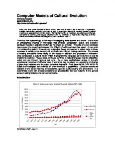
5.3 Initializing the Parameters The probability of death for a female peacock is directly proportional to its constitution and inversely proportional to its age. This suggests the health of a female peacock should be given by the function: health = constitution age : The probability of death for a male peacock is directly proportional to its constitution, inversely proportional to its age, and is modulated by a Gaussian function of its deviation from the optimal tail length. The health of a male peacock is given by the function: 2 health = constitution exp( ?(tail length ? optimal tail length) ) age c where c controls the eect of tail length on the health of male peacocks. When c = 1 the tail length has no eect on peacock health. As c decreases, tail length has an increasing eect on peacock health, with tails further from the optimal aerodynamic length lowering the value of health. The variable optimal tail length is set arbitrarily to 5 tail length units. The relative change in tail length is the important consideration for these experiments. A graph of male peacock health with constant constitution and a value of 10 for c is shown in 5.1.


22

Health Function for Males with Constant Consititution Health = constitution / age * exp(-(tail - optimal tail)^2 / c)

Health

constitution = 5 optimal tail = 5 c = 10

2 1.5 1 0.5

10 5

5 Age

Tail Length

10 15

0

Figure 5.1: Male Peacock Health

Each year, every peacock's health is evaluated and the peacock dies if:

health < random(threshold) where random(x) returns a random number in the range [0; x]. The starting population for these experiments was set to 1000 males and 1000 females. The starting population needs to be large enough so that the development of the population is not dominated by random drift caused by the pseudo-random number generator. When the population reaches a critical size, the value of the threshold is increased. This simulates competition for limited resources in the environment. The environment can only support a nite number of peacocks. The speed gene is a continuous valued attribute between the range 0 When this level is reached, the probability of death for each peacock increases, as resources become more scarce and competition becomes more intense. For this model, the critical size of the population is set to 4000. The genotype of a new peacock is created from its parents' genotypes by simply selecting each gene from one of the parents at random. The number of male peacocks in the female selection set is arbitrarily set to 16. The probability that a female participates in reproduction is set to 25%. The probability of mutation is set to 10%. When mutation occurs, the change in the gene value being mutated is 20% of the initial value for the population.


23

5.4 Results Figure 5.2 shows a typical result obtained when the health evaluator described above is used with c equal to 10. The graphs plot the average value of the male tail length gene and the female tail preference gene. Male Tail Length

Female Tail Preference

5.5

0.60

5.0 0.50

Tail Preference

Tail Length

4.5

4.0

0.40

0.30

3.5

0.20 3.0

2.5

0

1250 2500 3750 Generation

5000

0.10

0


5000

Figure 5.2: Male Peacock Tails Disappearing

The graphs indicate a downward trend in both tail length (in males) and tail length preference (in females), supporting the theory that genetically-based sexual preference in females can dominate simple survival considerations. Even though the optimal tail length is 5, when the average tail length preference in females drops below 0.5, the males respond with tails shorter than the optimum. The eect is that males with short tails pass their genes onto the next generation and the short-tail gene becomes dominant in the peacock community. The fact that short-tailed males are more successful than long-tailed males means that it becomes vital for females to select mates with short tails in order for their male ospring to also be successful. The two genes therefore exert pressure on each other and their values decrease until male tails have decreased to a value of approximately 3.25 tail length units, a 35% decrease. The dormant female tail length gene follows the trend of the active male tail length gene, even though this gene has no eect on the female. Similarly, the dormant tail length preference gene in males follows the active tail length preference gene in females. The


24

overriding consideration is that the success of a peacock depends not only on its own tness, but also on the tness of its ospring (and their ospring, etc.). The downward trend in tail length cannot continue unbounded. At some point, the consideration of survival overcomes the consideration of sexual attractiveness, to the extent that males with tails which are \too short" do not even survive to maturity and hence do not participate in reproduction at all. A male with a very short tail becomes so hopelessly un t that even though females prefer him to other males in the community, he dies before being able to propagate many/any of his genes into the next generation. When this occurs, males with longer tails pass on a greater proportion of genes to the next generation, forcing tail length to stabilize. The selective pressure for short tails (via the low female tail preference gene) ensures that male tail length remains at a low value. This is seen in the graphs as the levelling o in both male tail length and female tail preference. Figure 5.3 shows the alternative result, the development of male peacocks with extravagantly long tails. Male Tail Length


7.5

0.90

7.0 0.80

Tail Preference

Tail Length

6.5

6.0

0.70

0.60

5.5

0.50 5.0

4.5

0


5000

0.40

0


5000

Figure 5.3: Defying Natural Selection? - Male Peacocks Evolve Long Tails

This outcome is also predicted by the theory, for the same reasons as the previous scenario. The genetic basis of tail length in male peacocks and tailbased sexual preference in female peacocks leads to a situation where the values of


25

these genes exert pressure on each other and advance together at a geometricallyincreasing rate, even at a substantial survival cost to the males. In a similar fashion for short tails, male tail length cannot continue to grow unbounded. Males with extremely long tails cannot survive long enough to reproduce, and hence even though the preferred mates for females are males with long tails, they are unable to participate in reproduction because these males die before they reach sexual maturity. When this occurs, males with shorter tails pass on a greater proportion of genes to the next generation. Following the same argument for short tails above, selective pressure by females preferring long tails ensures male tail length remains high. Peacock constitution continues to grow throughout the life of the simulation. There is no bound on the value reached by this gene, since there are no ill eects on having a higher constitution value than the average. Figure 5.4 shows the typical result when the health evaluator described above is used with c equal to 10,000. Note that although a negative tail length is physically impossible, its the relative changes that are important in this discussion; if the optimal tail length constant had been set to a number in the order of thousands, a negative tail length would not occur. Male Tail Length


150

1.0

0.8

Tail Length

Tail Preference

50 0.6

0.4

-50

0.2

-150

0

2000 4000 Generation

6000

0.0

0


6000

Figure 5.4: The Simulation for a Large Value of Peacock Health Constant

Male peacock tail length and female peacock tail preference both increase rapidly over the rst 750 generations in accordance with Fisher's theory. Tail


26

length in males stabilizes for approximately 500 generations before dropping rapidly, following the decline in female tail preference. This appears to contradict the Fisher theory. Fisher proposed that male tail length would increase in tandem with female preference until an equilibrium was reached. In this scenario, no equilibrium position is sustained. The system oscillates between two con gurations; one con guration for large male tail length and high female tail preference and the other con guration for small (largely negative) male tail length and low female tail preference. A small equilibrium period is realised in between cycles of rapid growth and rapid decline of the two gene values. Smith [12] proposes a theory that provides a possible solution to this apparent contradiction. He explains how small populations can pass from one adaptive peak to another through a selectively inferior intermediate. That is, a small population can move from one local maximumto another local maximumthrough an intermediate minimum. In the case of the peacock model local maxima, occur when male tail length matches female tail preference. The key to this theory is that the population must be small. In large populations, selective pressure forces any deviation from the local maxima back, since members of the population which deviate from the maximum value (i.e. at the intermediate local minimum) are penalized and not selected for further generations by the females of the population. Small populations can allow this transition, since there is limited competition for mates. There are little or no sexually attractive males in the population, so females lower their standards and select a mate from the sexually unattractive males. The lower the number of sexually attractive males, the greater the probability an unattractive male is chosen as a mate and hence the greater the probability that the transition can be made. Figure 5.5 shows the number of sexually mature males for a value of c equal to 10000 and for a value of c equal to 10. For a value of c equal to 10, the number of sexually mature males in the population is always greater than 1000. In this case, no transition from one maximumto another is evident. The number of sexually mature males approaches and reaches zero for a value of c equal to 10000. When the sexually mature population is small, transitions from one maximum to the other are evident. This supports Smith's theory which provides an explanation for the transition from one local maximum (high preference and large tail length) to another (low preference and small tail length) through a local minimum (low preference and large tail length) and back again. Figure 5.6 shows a three dimensional plot of male tail length, female tail preference and the number of sexually mature males. The system starts at a con guration of average female tail preference/optimal male tail length. The number of sexually mature males quickly increases as the system stumbles around the unstable equilibrium start con guration. This is the vertical line in the center of Figure 5.6. Finally, female tail preference starts heading upwards; male tail length quickly starts to increase in an attempt to satisfy the female population. An optimal value, approximately equal to 0.94,


27

3000

Number of Sexually Mature Males

c = 10000

c = 10

2000

1000

0

0

1000


4000

5000

Figure 5.5: The Number of Sexually Mature Males for Dierent Values of the Peacock Health Constant

for female tail preference is quickly reached; average female tail preference cannot increase past 1.0. Male peacock tail length continues to increase. As this occurs, the number of sexually mature males decreases since having a higher tail length implies having a higher probability of dying. Finally the local maximum con guration of 0.94 for female tail preference and 122 for male tail length is reached. For lower values of c, the system remains in this local maximum con guration, however for high values of c, a transition to another local maximum occurs. The local maximum points occur at the con gurations high female tail preference/long male tail length and low female tail preference/short male tail length. These points are diagonally opposite each other in Figure 5.6. The transition through local minima is the path on the curve from one local maximum to the other. The horizontal line from high female tail preference to low female tail preference (with male tail length remaining mostly constant) occurs when there is a low number of sexually mature males. This transition only occurs when there is a low number of sexually mature males, as described by the Smith theory introduced earlier. When female tail preference falls below 0.5, a selective downward pressure on male tail length occurs. Male tail length starts to decrease. As male tail length becomes closer to the optimal tail length, the number of sexually mature males increases, reaching a maximum value at or around optimal


28

Sexually Mature Males 2500 2000 1500 1000 500 0 0.8 0.6 -100

-50

0

Male Tail Length

50

100

0.4 0.2 Female Tail Preference

Figure 5.6: Relationship Between Male Tail Length, Female Tail Preference and Number of Sexually Mature Males

tail length. Selective pressure continues to force tail length down. A new local maximum con guration at 0.05 for female tail preference and -118 for male tail length is reached. At this stage the number of sexually mature males is signi cantly low, a transition through a dierent local minimum back to the original local maximum occurs. This process continues; the system cycles between these two local maximum con gurations - a type of attractor resulting. Table 5.1 shows the percentage increase of male peacock tail length for different values of c. The table indicates that the percentage change of male tail length is dependent on the value of the constant c. In nature, male peacock tail length is approximately two to three times that of female peacock tail length. This corresponds to a value of c approximately equal to 75. Obviously, values of c greater than 1000 do not model peacock evolution on Earth. However, an examination of these models with high values of c, allows exploration of alternate universes; universes in which our improbable is their highly probable.


29

Value of c Percentage Increase in Tail Length 1 0% 5 20% 10 35% 20 65% 50 110% 100 180% 1000 720% 10000 2300% Table 5.1: Percentage Increase in Male Tail Length for Dierent Values of Peacock Health Constant

5.5 Conclusions Fisher's theory submits that apparently counter-adaptive phenotypic traits (i.e. male peacocks' tails) can arise simply due to the fact that both sexual attractiveness in males and sexual preference in females have a genetic basis. Simulation of the salient aspects of this scenario is achieved quickly and easily, by deriving minimal genotypes and phenotypes of male and female peacocks using the general evolutionary model. The general framework manages the interactions between these entities and all other aspects of the simulation. The experiments with this model con rm that Fisher's theory is adequate to explain the observed development of peacocks. For low values of the peacock health constant, c, the constructed model supports Fisher's theory exactly. For high values of c, the feed-forward pressure on both the sexual attractiveness and sexual preference gene as described by the Fisher theory is evident, but equilibrium of the two genes is not apparent. Instead, the system oscillates between two local maximum con gurations. Smith's theory explains how small populations can make transitions from one local maximum to another through a local minimum. For high values of c, the number of sexually mature male peacocks approaches zero. Smith's theory appears sucient to explain these transitions.

CHAPTER 6

Extending the Model The basic model de ned in chapter 4 has two major de ciencies. This chapter examines the extensions made to the basic evolutionary model to allow simulations of organism interactions with their environment and organism interactions between dierent species.

6.1 Limitations of the Basic Generalized Model Features not realized in the rst model: interaction between phenotypes and their environment, and interaction between dierent species.

6.1.1 Environment Interactions

In the basic model, phenotype interaction with the environment can only be modelled by incorporating probabilistic measures in the overridden functions. For example, the function determining the probability of death of a phenotype may incorporate a probability of a food shortage occurring, thus making the probability of death for each phenotype slightly greater. This is sucient for simple models, but more complex models require an explicit representation of the environment in which species evolve. Ideally, a de nition of a new base class where the environment is modelled as a grid of cells, each with attributes describing the state of the environment in its locality is required. The user-de ned functions will have the ability to examine and/or modify these attributes.

6.1.2 Species Interactions

The framework needs to be extended to support populations of several species. The basic model only allows phenotype interactions between dierent types of organisms to be modelled by some probabilistic measure in the user de ned functions. For example, the probability of death function may have some probability that a phenotype is preyed upon by a predator, and hence dies immediately. The 30

6. Extending the Model

31

framework must allow for phenotypes to directly kill other phenotypes of the same species or of diering species. This allows the study of interactions between dierent species, for example predator/prey scenarios and parasitic/symbiotic dependencies.

6.2 Enhancements to the Basic Model 6.2.1 The World Class

A world class is de ned that models the environment that organisms live in. The world is de ned as a two dimensional array of cells. Cells can be arbitrarily large or small depending on the scenario being modelled. The environment is then a global variable of type world. Each cell contains the following attributes: int x position { the horizontal position of the cell in the world, int y position { the vertical position of the cell in the world, and objectlist *members { a list of organisms currently residing in this cell. WORLD

Y

X CELL Cell Attributes X Position Y Position List of organisms

Figure 6.1: The Global World Class

Model speci c information relating to the state of the environment (in each cell) is added as attributes of the cell class. Cell attribute access can either be private or public; access control is determined by the user. The cell class requires the following functions to be de ned:


32

void initialize();

This function initializes the state of the environment, by initializing all the cell attributes. Model speci c cell attributes are initialized in this function. This function is called at the beginning of each new simulation.

void update(int generation);

This function updates the state of the environment in each cell each generation. The model speci c cell attributes are modi ed in this function to simulate changes in environment state. This function is called at the end of every generation. The world class provides the following member functions:

cell *get cell(int x, int y);

This function returns a pointer to the cell at horizontal position x and vertical position y. If one or both ordinates is not valid, NULL is returned. This function is used to access cell attributes for each cell in the environment.

void initialize world();

This function initializes all the cells in the environment. Each cells' initialize member function is called. This function is called at the beginning of the each new simulation.

6.2.2 Changes to the Individual Class

The individual class requires another three functions to be overridden in derived classes:

void move(int *x, int *y);

This function determines the cell an organism is to move into. Phenotype attributes such as probability of moving along with environmental attributes such as food in cell, are likely to aect the behaviour of this function. The parameter *x returns the horizontal position of the cell the organism moves into. The parameter *y returns the vertical position of the cell the organism moves into. If the organism is not to move in the current breeding cycle, the existing position is returned. This function is called every breeding cycle for each organism.

void initial position(int *x, int *y, int xp1, int yp1, int xp2, int yp2);


33

This function determines the cell that a new organism is born in. When a new organism is created, the initial position of the organism is found by calling this function. The parameter *x returns the horizontal position of the cell the organism is born in. The parameter *y returns the vertical position of the cell the organism is born in. The xp1 and yp1 parameters represent the horizontal and vertical positions respectively of the female parent's cell. Similarly, the xp2 and yp2 parameters represent the horizontal and vertical positions respectively of the male parent's cell. For asexual populations, the second pair of cell positions is ignored. This function is called for each new organism at the time it is created.

bool kill individual(individual *i);

This function determines if the current organism kills the organism passed as a parameter. Attributes of both organisms are expected to determine the outcome of this function. If the organism passed as a parameter is killed, the function returns true, else false is returned.

6.2.3 Changes to the Population Class

The population class provides the following new member functions:

void move(int generation);

This function allows organisms to move from one cell to another. It rst calls the move member function for each organism. If the return position is dierent to the organism's current position, the organism moves from its current cell to the cell given by the return position. When the organism moves out of a cell, the organism is removed from the member's objectlist for that cell. When an organism moves into a new cell, the organism is added into the member's objectlist of the new cell. The current position of the organism is updated accordingly. If the return position is exactly the same as the current position, the organism does not move.

void interact(int generation, int *males reproduced, int *females reproduced, int *males killed, int *females killed);

This function models organism interactions between organisms of the same species and organisms of dierent species. The choose encounter set member function of the sexual population class (this was previously the choose selection set function in the basic model) is called to determine the list of organisms encountered by the organism in this breeding cycle. The function calls the participate in reproduction member function for each female organism in the population. A return value of true, indicates the female reproduces in this breeding cycle. A mate is then chosen by


34

calling the choose mate member function. If a mate is chosen, a new organism is created, and the genotype and phenotype of the ospring are created by calling its reproduce and develop member functions. The parameters *males reproduced and *females reproduced are assigned the number of males and females born in this breeding cycle. Each organism in the encounter set (as selected by choose encounter set member function) is passed as a parameter to the kill individual member function. If this function returns true, the organism passed as a parameter is killed and deleted from the population list, else it survives into the next generation. The parameters *males killed and *females killed are assigned the number of males and females killed in this breeding cycle. Pseudo code for the main loop of the evolutionary model is given in Appendix B.

CHAPTER 7

The Predator/Prey Model The extended evolutionary model described in the previous chapter is now used to simulate predator/prey relationships. We use the features of the extended model to investigate population dynamics and variations in a genetically determined defensive strategy of the prey.

7.1 Foxes and Rabbits Taylor [13] describes an ecosystem that contains two living entities, foxes and rabbits, and one environment attribute, grass. Grass grows throughout the environment, growing at a uniform constant rate. It acts as an environmental attribute, not modelled as a living entity, and is only present in the model to act as food for rabbits. The foxes prey on the rabbits and the rabbits consume the grass in the environment. Both foxes and rabbits have a health attribute that acts as a general indicator of the animal's well-being. An animal whose weight goes below a lower threshold dies from starvation. Only animals with a health value above a higher threshold can participate in reproduction. When reproduction occurs, the health of the new ospring is set to the average of the health of the two parents. Both parents lose a xed amount of health after reproduction. Rabbits gain health by eating grass. Foxes gain health by preying on rabbits. Both animals are endowed with a characteristic metabolic rate, that causes them to lose a certain percentage of their health each time cycle, independent of what else happens in their lives that time cycle. As a consequence, both animals must eat regularly in order to avoid starvation. Only animals that are able to eat more than enough to oset the metabolic rate will participate in reproduction. Both foxes and rabbits can move one cell in any direction each time cycle (assuming eight connectedness of cells). Both types of animals can examine the environment for food and enemies in their current cell. Without predation, it is expected that the rabbit population will rapidly increase and then stabilize around the carrying capacity of the environment, which is determined by the rate of growth of the grass. With predation, the numbers of 35

7. The Predator/Prey Model

36

foxes and rabbits tends to oscillate, as illustrated by many mathematical models; one such model is described by Boyce [2]. However, classical mathematical models simply model population behaviours. It is important to note that this simulation is complicated by the fact that the animals have genetically based survival mechanisms. A Rabbit contains a speed gene that controls its ability to elude foxes. The speed gene is a continuous valued attribute in the range [0; 1]. Rabbits with a relatively high value for the speed gene are better able to avoid being preyed on by foxes, but have a faster metabolism (they require more energy) and hence must eat correspondingly more food in order to avoid starvation. Rabbits with a lower value for the speed gene can participate in reproduction more often, since they don't use up as much health each time cycle due to their lower metabolic rate, but are more vulnerable to being eaten by predators. Foxes also contain a speed gene that controls the ability to capture rabbits. The speed of both animals (the physical manifestation of the speed gene) determines if a fox captures a rabbit or if the rabbit eludes the fox.

7.2 De ning the Simulation Both the fox and rabbit genotypes are represented by two attributes: 1. health { a measure of the general well-being of the animal, and 2. speed { a measure of how well the animal can elude predators or capture prey. There is a 1-1 mapping from genotype attributes to phenotype attributes. That is, phenotype attributes are the physical manifestation of the genotype attributes. Phenotypes are represented by the two attributes: 1. health, and 2. speed. Each cell in the environment contains one attribute: 1. grass { the amount of food available in the cell for the rabbits to eat. Each time cycle, the grass attribute is incremented by a constant amount to simulate growth of grass in the environment. The grass attribute is initialized to 100, and is incremented by 50 each time cycle. The initial population is assigned a health attribute value of 100. Each time cycle, fox and rabbit health is decreased by: a + b speed where the constants a and b control the cost of survival in the environment; a corresponds to the metabolic rate, b a constant survival cost independent of


37

metabolic rate. For both types of animals, a and b is set to 10. Hence for a rabbit whose speed gene is 0.5, 15 is deducted from the health attribute each time cycle. Each time cycle, rabbits eat a proportion of the grass in its current cell. The rabbit's health increases by:

min(max gain; grass in cell) where max gain is the maximum health gain that can be obtained by a rabbit each time cycle (the maximum grass that can be eaten). The max gain variable is set to 15. Animals die if: health < survival threshold The survival threshold is set to 25. For a particular animal, the set of animals encountered in each time cycle is set to be the neighbouring animals in its cell. This encounter set is all the animals a particular animal may reproduce with or prey on in the current time cycle. That is, animals may only reproduce or prey on animals in its current cell. Reproduction occurs if the two encountering animals both have: health > reproduction threshold The reproduction threshold is set to 50. After reproduction, each parent's health is reduced by 15. The mature age for a fox and a rabbit is set to 5 time cycles. Immature animals are excluded from the reproduction process. The new ospring is born in the same cell as its parents. Each time a fox and a rabbit encounter each other, the fox kills the rabbit if: random(speed of fox) > random(c speed of rabbit) where random(x) returns a random number in the range [0; x], and c controls the number of rabbits a fox can prey on. The value of c is set to 15. If a fox successfully preys on a rabbit, the fox's health is increased by: min(max gain; 21 health of rabbit) where max gain determines the maximum increase in health possible for eating a rabbit (there is a limit to how much can be eaten at one kill). The max gain variable is set to 50.

7.3 Results Figure 7.1 shows the typical results obtained from a simulation with the parameters de ned as in the previous section. The initial rabbit population was set


38 Predator-Prey Model

0.60

Rabbit Speed Gene

Rabbit Population

18000

12000

6000

0

0


0


1000

0


1000

6000

Average Grass

Fox Population

0.20

0.00

1000

800

533

266

0

0.40

0


1000

4000

2000

0

Figure 7.1: The Cyclic Nature of the Predator/Prey Model

to 2000, with the initial fox population set to 1000. All animals were randomly distributed over a 20 20 world. The ecosystem behaves similarly to the Taylor simulation it was based on, in that the rabbit population oscillates with the fox population, though slightly out of phase. As the number of rabbits increases, the number of foxes tends to increase since there is a greater source of food for the foxes to prey on. More foxes survive longer, allowing a greater proportion of foxes to participate in reproduction, hence causing a rise in the fox population. As the number of foxes rise, the number of rabbits starts to decline due to the increased number of predators, increasing the probability of dying for rabbits. The fall in rabbit population creates a food shortage amongst the fox population, causing the fox population to decline in numbers. As long as the rabbit population is not made extinct, the fall in


39

the number of foxes leads to a greater probability of surviving amongst rabbits, leading to an upsurge in the the rabbit population. This cyclic motion can occur inde nitely, provided that neither population becomes extinct. The speed gene in rabbits follows the trend in fox population, though out of phase. Evolutionary change requires many generations to take hold and hence, genetic variation is expected to be out of phase with population dynamics. When the number of foxes in the community is small, rabbits with low speed gene values prosper since they do not spend as much health each time cycle meeting the metabolic rate. Low speed gene rabbits are above the reproduction threshold more often than the high speed gene rabbits and hence participate more often in reproduction, causing a greater proportion of future generations to have a low speed gene. Although these rabbits have a greater probability of being preyed on, there is very few predators around, so the risk of being killed is minimal. As the number of foxes rises there is a genetic pressure on the speed gene in rabbits to rise. Although it is advantageous to have a low speed gene value (less health is used in each time cycle), when the fox population is high, the probability of dying for rabbits is much greater, resulting in rabbits with low speed genes being killed more often than rabbits with high speed genes. As a result, a greater proportion of rabbits with high speed gene values survive and participate more in reproduction causing a general rise in speed gene values in the future rabbit generations. The average grass remaining in each cell is seen to vary with the number of rabbits. As the number of rabbits increases towards a local maximum, the average grass remaining in each cell approaches zero. An increase in the average grass remaining is evident when the number of rabbits starts to fall. Since only the rabbits in the ecosystem consume the grass, the change in the grass remaining is dependent only on the number of rabbits. The mathematical model described by Boyce predicts the observed result. Formulating the problem into dierential equations, the mathematical model suggests two possible solutions, one in which both populations die out, and another in which a cyclic trend (as described above) occurs. The mathematical model does not predict any genetic trends; this would require another series of dierential equations to be solved. Although the mathematical model can be used to solve this problem, the real advantage in using the general framework is that it provides a precise de nition of the evolutionary process in which problems too complex for traditional mathematical methods can be de ned. Figure 7.2 shows the results obtained from a simulation de ned above with no predators. The initial rabbit population was set to 2000, randomly distributed over a 20 20 world. With no predation, the rabbit population grows unbounded until the maximum carrying capacity of the environment is reached. At this time, the average grass remaining in each cell approaches zero, since all the new grass grown in the current cycle is consumed by the rabbit population. Initially, when the rabbit population is below the maximum carrying capacity of the ecosystem, and hence


40 Predator-Prey Model 0.60

Rabbit Speed Gene

Rabbit Population

3000

2000

1000

0

0


0


1000

0


1000

Average Grass

400

66.7

Rabbit Health

0.20

0.00

1000

100.0

33.3

0.0

0.40

0


1000

267

133

0

Figure 7.2: The Predator/Prey Model with No Predators

not all the grass is being consumed, the average grass remaining in each cell increases rapidly. At some point, the rabbit population increases to a number which exceeds the rate of regrowth of grass, and the supply of grass is consumed. This corresponds to a fall in the average grass remaining, decreasing steadily to zero. With no predators, the probability of being preyed on is zero, so having a speed gene value above zero is unnecessary and a disadvantage since it requires using more health each time cycle meeting the metabolism rate. Rabbits with a low speed gene are above the reproduction threshold more often than rabbits with a high speed gene, and hence participate more often in reproduction. This results in a greater proportion of future generations having a low speed gene value.


41

When the supply of grass is plentiful, the health of rabbits increases because the health gained by consuming grass is greater than the health cost of the metabolism rate. When the built up supply of grass (grass not eaten in previous generations) is consumed, the amount of remaining grass becomes limited. Competition amongst the rabbits occurs and rabbits receive a restricted amount of grass each time cycle. This corresponds to a drop in rabbit health. The grass in each cell is increased by 50 each time cycle. After generation 500, rabbit speed is approximately zero. This corresponds to a decrement in rabbit health of a + b speed = 10 + 10 0:0 = 10 each time cycle. This would suggest that the maximum carrying capacity of the ecosystem would be grass increment = (20 20) 50 number of cells health decrement 10 = 2000 rabbits. However, experimentation shows that a population of approximately 2800 rabbits (7 per cell) can be supported by the system. Each time cycle, the rabbits in each cell are randomly shued and chosen in this order to consume their share of the grass. During this consuming period, as discussed earlier, a rabbit will consume min(max gain; grass in cell) grass units. It is not the case that an equal share of grass in the cell is given to each rabbit. For example, if the cell contains 7 rabbits (with a zero speed value), has 3 grass units in supply, and is incremented by 50 grass units each time cycle, three rabbits would have their health incremented by 5, one rabbit would have its health decremented by 2 and three rabbit's health would be decremented by 10. On average, the health of each rabbit in the cell would be decremented by 507 7 units; indicating that each rabbit will eventually die. The rate of decrement in health is slow enough to ensure that reproduction can occur (by the rabbits who have had a positive increment in health that time cycle), and that new rabbits be born into the ecosystem. It appears that an equilibrium between rabbit death and rabbit birth rates is obtained when 7 rabbits, on average, occupy each cell. Figure 7.3 shows the results obtained from the simulation with the value of a set to 5. All other parameters were set as above. The initial fox population was set to 1000, the initial rabbit population set to 2000. A 20 20 world was used, with the initial populations of both species randomly distributed over its range. Initially, the ecosystem cycles between stages of a high rabbit population and a low rabbit population, as seen in Figure 7.1 and discussed earlier. However, after generation 3000, both the rabbit population and the fox population have stabilized. After this time, the cyclic trend appears to have ceased. Both rabbit speed gene and fox speed gene values tend to rise over this equilibrium period. Foxes with a high speed gene value are able to hunt more prey


42 Predator-Prey Model 0.70

Rabbit Speed Gene

Rabbit Population

6000

4000

2000

0

0


5000

667

333

0

0.50

0.40

0


5000

0


5000

1.00

Fox Speed Gene

Fox Population

1000

0.60

0


5000

0.80

0.60

0.40

Figure 7.3: Stabilization Within the Predator/Prey Model

and survive longer than foxes with a low speed gene value, hence participating in reproduction more often, causing future fox generations to acquire the high speed gene value. Although it is a disadvantage, an increase in the rabbit speed gene is necessary to counteract the increase in the fox speed gene. An equilibrium is reached and the two populations remain stable. Using the general framework introduced in this report, experimentation indicates that a stable equilibrium between predator/prey populations is possible. A result not indicated by the Taylor model, and only suggested as feasible in the mathematical model, but evident in nature.

CHAPTER 8

Conclusions 8.1 The General Model A general framework was de ned for the process of evolution which abstracts the invariant parts of the evolutionary process and allows a programmer to model particular situations by instantiating the variant parts of the process. The invariant parts are controlled by the framework. Only problem speci c information is required to perform the simulation. This allows the programmer to focus easily on the aspects of the process which are deemed relevant in a particular experiment. The inheritance mechanism provided by the C++ class structure was used to de ne particular species as derivations of general base organisms. Simulation of a particular scenario is achieved by deriving minimal genotypes and phenotypes of male and female organisms speci c to the simulation. The general framework manages the interactions between these entities and all other aspects of the simulation, hiding all the implementation details used to control and manage the large number of objects in the model. This gives the user the freedom to model evolutionary scenarios without being concerned with the underlying control structure. Since none of the internal implementation details need be known, users with only limited programming skills can tackle complex evolutionary problems quickly and easily. The C++ function overriding mechanism allows the general framework to be viewed from dierent abstraction levels. Apart from the several model speci c functions that need to be de ned in derived classes, users can override any of the controlling functions to modify the calling structure of the evolutionary process allowing great exibility in modelling of evolutionary simulations. The power of the general framework is that it provides a simple method of modelling evolution in computers. Organisms exist inside the computer memory; they interact, reproduce, ght, die, give birth and develop, just as in nature. Mathematical models cannot model these individual interactions. A precise language is de ned under the framework that allows problems too complex for traditional mathematical models to be de ned. Mathematical models cannot describe the evolutionary process, whereas the framework provides a clear de nition. 43

8. Conclusions

44

8.2 Future Extensions The general framework as de ned operates sequentially. To avoid bias in the simulation, each population is randomly shued before organisms are processed in turn. However, natural systems behave concurrently. There is no sense of sequential ordering in nature; organisms interact with each other and the environment concurrently. One organism does not wait for another organism to nish moving before it participates in reproduction. Organisms are independent of each other; sequential processing forces a dependency on an organism to wait for others. To better model natural systems, the general framework needs to be concurrent. Large simulations (in the order of 10000 organisms) require a long period of time to complete using the sequential version of the evolutionary model. A concurrent version not only models nature better, but will provide a solution in a quicker period of time. Using a massively parallel machine, large complex simulations can be completed in a relatively short period of time. The general framework is implemented using C++. To build a simulation, users must provide de nitions of model speci c genotypes and phenotypes. Several functions need to be overloaded in the new derived classes. Users must have knowledge of C++ to do this. It should be possible to create a simple language consisting of keywords representing distinct parts of the evolutionary process. For example, the reproduction process could be represented by the string: \Ospring = REPRODUCE Parent1 Parent2". With a simple interface, the building a complex biological simulation can be reduced to a point-and-click process, suitable for the intended inexperienced users.

References 1. R. K. Belew. Arti cial Life: A Constructive Lower Bound For Arti cial Intelligence, IEEE Expert , Vol. 6, Iss. 1, pp. 8-15, January 1991. 2. W. E. Boyce, R. C. DiPrima. Elementary Dierential Equations and Boundary Value Problems , Edition 4, John Wiley and Sons, pp. 493-497, 1992. 3. C. Caldwell, V. S. Johnston. Tracking a Criminal Suspect Through FaceSpace with A Genetic Algorithm, Proceedings of the Fourth International Conference on Genetic Algorithms , International Society for Genetic Algorithms, pp. 416-421, 1991. 4. R. Dawkins. The Blind Watchmaker , Harlow, 1986. 5. R. Dawkins. The Evolution of Evolvability, Arti cial Life, SFI Studies in the Sciences of Complexity , Addison-Wesley, 1988. 6. R. Dawkins. The Extended Phenotype , Oxford University Press, 1983. 7. R. Dawkins. The Sel sh Gene , Oxford University Press, 1976. 8. R.A. Fisher. The Genetic Theory of Natural Selection , Oxford Clarendon Press, 1930. 9. I. Pohl. C++ for C Programmers , Benjamin/Cummings Publishing Company, 1994. 10. T. S. Ray. Evolution, Ecology and Optimization of Digital Organisms, Arti cial Life 1 , Addison-Wesley, 1987. 11. T. S. Ray. An Evolutionary Approach to Synthetic Biology: Zen and the Art of Creating Live, Arti cial Life 1 , Addison-Wesley, 1987. 12. J. M. Smith. Did Darwin get it Right?: Essays on Games, Sex, and Evolution , Penguin Books, 1993. 13. C. E. Taylor, D. R. Jeerson, S. R. Turner, S. R. Goldman. RAM: Arti cial Life for the Exploration of Complex Biological Systems, SFI Studies in the Sciences of Complexity , Ed. C. Langton, Addison-Wesley, 1988. 45

Bibliography 14. S. Windybank. Wild Sex , Reed Books, 1991.

46

APPENDIX A

Original Honours Proposal Title: Computer Modelling of Evolution Author: Luigi Barone Supervisors: Dr. Philip Hingston and Dr. Lyndon While

Aim This project will model evolution via natural selection. Modelling of evolution will encompass a whole community of organisms, interacting with each other and their environment. Natural selection is the driving force behind evolution and as such should guide the way in which the organisms develop. The forces dictating development and success of organisms should become evident from the simulation; they should not be encoded into the model. This project will examine these forces behind natural selection and attempt to establish a general model for evolution. Dawkins, in his Blind Watchmaker program [1,2], has attempted to model the process of evolution. He models the processes of reproduction and development, in which genotypes are transformed into phenotypes. In his program, the choice of successful phenotypes is left to user selection. This is arti cial selection, not natural selection; the user is specifying which phenotype is chosen as the parent for the next generation. Since evolution involves the process of natural selection, as opposed to arti cial selection, this constitutes a major weakness in his model of evolution. Dawkins recognizes this problem in his book [2] and presents the challenge of providing a complete computer model for interactions between organisms. This is the ultimate goal for this project. Instead of modelling evolution of a simple organism as in the Dawkins program, this project will model communities of organisms. Interactions between organisms will be examined, as will sexual reproduction. Dierent mechanisms of combining parent genes during the reproduction process will be tested. The Dawkins model provides a simplistic, user guided, evolution process. The development of 47

a more realistic model, which has interactions between organisms with natural selection is the essence of this project.

Background Evolution is the study of how complex organisms developed from the single celled organisms that came into existence after the creation of the Earth. In natural systems the total genetic package of an organism is called the genotype. The organism formed by the interaction of the genotype with the environment is called the phenotype. Phenotypes contain entities, called genes, that are capable of selfreplication. Genes are passed on to ospring during the process of reproduction. Any inexact replication of genes during reproduction generates ospring which dier from their parent(s) in an unexpected manner. This is called mutation. At every generation, the genes of each organism in uence the composition of the phenotype. The success of the phenotype in its natural environment determines whether the genes it contains go forward into the next generation. The greater the success of a phenotype, the greater the probability the phenotype will participate in reproduction. With asexual reproduction, the ospring inherits genes (all from its parent) that have produced a long line of successful phenotypes, since failed phenotypes do not pass on genes. For sexual reproduction, ospring receive some combination of genes from their parents, which have been successful as phenotypes in the past. Natural selection is the process by which the more successful phenotypes of a generation pass on a greater proportion of genes to the next generation. In other words, natural selection suggests that any adaptation (through an organism's genes) that helps an organism to survive and produce more ospring will eventually become dominant in the organism community, because more ospring that contain this adaptation will be produced. As a consequence of natural selection, phenotypes pass on genes which have produced successful organisms previously, to their ospring. The process of evolution is shown graphically in Figure A.1.

Method An initial phase of this project is to develop a model for the genotypes of organisms. Each gene in the organism will have a speci c role in the development process of phenotypes. That is, each gene is directly related to some behaviour in its corresponding phenotype. Dawkins used nine genes in his original model to control how each organism was drawn. This works well when there is no contact between dierent organisms, but in this project, phenotype interactions are to be modelled, so genes will be needed that have an in uence on how the organism behaves in its community (for example, a gene that controls how friendly a phenotype is to its neighbours could be introduced). The establishment of a complete description of genes that can be used to model organisms and their interactions will be a signi cant part of this project. 48

Generation One

Genotype 1

DEVELOPMENT

Phenotype 1

Genotype 2

DEVELOPMENT

Phenotype 2

unsuccessful DEATH phenotypes

Genotype N

DEVELOPMENT

Phenotype N

successful phenotypes

REPRODUCTION

of genotypes

Generation Two

Figure A.1: Computer Model of Evolution

Once genotypes have been established, a development process that transforms genotypes into phenotypes is required. Each gene value of the genotype directly aects an attribute of the phenotype (be it appearance, sex, friendliness, etc.). This function takes the encoded information in an organism's genes and transforms it to produce a new organism. There is a direct correspondence between how this function will behave and what the genes of the organism represent. The tasks of establishing a gene description for organisms and a function to translate the gene description to produce a phenotype will need to be designed with each other in mind. Natural selection is the process by which organisms that are better equipped to survive in their environment pass on their genes to their ospring. The more successful an organism is, the greater the chance the ospring of the organism will survive and reproduce. For each phenotype, in each generation, some ` tness' value must be assigned to it, that indicates the successfulness of the organism in relation to the other organisms in its generation. A simple tness function (as used in most genetic algorithms) will not be sucient to model the complex interactions between organisms. Some mechanism of evaluating success of an organism will need to be devised. The development of this stage of the project 49

will require modelling how organisms interact with each other. A reproduction process that passes on genes from one generation to another is needed. This function must produce new organisms from the most successful organisms of the previous generation. The genes of the parent organisms need to be combined in some way to produce the genes in the ospring. One mechanism for combining genes will be used initially and then other methods will be tested. Replication of genes in organisms is never guaranteed to be error free; there is some chance that an error may be introduced during the copying of parent genes to ospring. This mutation will need to be incorporated into the model of evolution. The project will attempt to model the evolution process by successively building up a nal general model. Dawkins [3] poses the question of how male peacocks developed long tails. This seems to contradict the natural selection principle, because a long tail is more of a hindrance to a peacock (e.g. it is harder for the peacock to run away from predators) than a short tail. One theory submits that long tails became dominant in peacocks, because female peacocks preferred long tails to short tails. This would give male peacocks with long tails an advantage over peacocks with short tails, because females are more likely to reproduce with long tailed peacocks than short tailed peacocks. Modelling this situation, using four simple genes (one each for tail length, sex, the tness of the peacock, and the preference for long tails) is being used as a basis for establishing an overall model of evolution via natural selection.

References 1. R. Dawkins. The Blind Watchmaker , Harlow, 1986. 2. R. Dawkins. The Evolution of Evolvability, Arti cial Life, SFI Studies in the Sciences of Complexity , Addison-Wesley, 1988. 3. R. Dawkins. The Sel sh Gene , Oxford University Press, 1976.

50

APPENDIX B

Pseudo Code for the General Evolutionary Model Pseudo code for the main loop of the evolutionary model is given below. for each species do initialize population; for each cell in the world initialize cell; for each generation do begin for each species do randomly shuffle population; for each species do for each individual of species do begin increment the age of individual; update phenotype of individual to simulate aging; end for each species do for each individual of species do if individual should die of natural causes then remove individual from population list; for each species do for each individual of species do begin find new cell to occupy; if new cell is different to cell of residence then move to new cell; end for each species do for each individual of species do begin determine encounter set; if individual wishes to participate in reproduction then

51

begin choose mate from encounter set; produce new genotype from parent(s) genotypes; develop genotype into a phenotype; add new individual into the population list; end for each individual in the encounter set if first individual preys on individual encountered then remove individual in encounter set from population list; end for each cell in the world update cell; end

52