Computer Vision Based Wheel Sinkage Detection for Robotic Lunar Exploration Tasks GuruPrasad Hegde, Christopher J. Robinson, Cang Ye, Senior Member, IEEE, Ashley Stroupe, Edward Tunstel, Senior Member, IEEE
Abstract— This paper presents a wheel sinkage detection method that may be used in robotic lunar exploration tasks. The method extracts the boundary line between a robot wheel and lunar soil by segmenting the wheel-soil images captured from a video camera that monitors wheel-soil interaction. The detected boundary is projected onto the soilfree image of the robot wheel to determine the depth of wheel sinkage. The segmentation method is based on graph theory. It first clusters a wheel-soil image into homogeneous regions called superpixels and constructs a graph on the superpixels. It then partitions the graph into segments by using normalized cuts. Compared with the existing methods, the proposed algorithm is more robust to illumination condition, shadows and dust (covering the wheel). The method’s efficacy has been validated by experiments under various conditions.
M
I. INTRODUCTION
OBILE robots are being used extensively in planetary exploration tasks. An important issue in such tasks is robot mobility. Sufficient traction from wheel-terrain/soil interaction is the key to maintain effective robot mobility. In general, a hard terrain produces larger traction than a soft terrain and thus better mobility. When moving on a soft terrain, a robot’s wheels may slip and/or sink into soil and experience traction loss. Excessive wheel sinkage may result in total traction loss and make the robot immobile. In other words, the efficiency of robot mobility depends on effective wheel-terrain interaction and wheel sinkage information can be used by a robot to assess the effectiveness of wheel-soil interaction and apply corrective action to mitigate the ill-effect of soft soil on the robot mobility. Almost the entire lunar surface is covered with regolith that contains fine soil grains (less than 1 cm in diameter) and much finer dust (less than 100 m in diameter). The thickness of the regolith varies with location from 2 meters to 20 meters. The properties of lunar regolith are very different from that of the soil of Earth or Mars. To effectively operate a robotic system on the lunar terrain, G. Hegde and C. Ye are with the Department of Applied Science, University of Arkansas at Little Rock, Little Rock, AR 72204, USA (phone: 501-683-7284; fax: 501-569-8020; e-mail:
[email protected]). C. J. Robinson is with the Department of Systems Engineering, University of Arkansas at Little Rock, Little Rock, AR 72204, USA (email:
[email protected]). A. Stroupe is with the Advanced Robotic Control Group, Mobility and Robotic Systems Section, Jet Propulsion Laboratory, Pasadena, CA 91109, USA (e-mail:
[email protected]). E. Tunstel is with the Space Department at the Johns Hopkins University Applied Physics Laboratory, Laurel, MD 20723, USA (e-mail:
[email protected]). This work was supported in part by NASA under a NASA EPSCoR RID Award and a NASA EPSCoR Award.
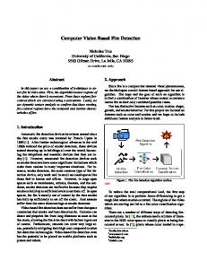
the effects of lunar dust must be addressed first. The Apollo missions have revealed that lunar dust has severe degrading effects on extravehicular activities. The Apollo astronauts cited multiple problems caused by lunar dust that adversely affected their activities on the lunar surface. Apollo astronaut John Young regarded dust as “the number one concern in returning to the moon.” For robotic surface operation, these effects include vision obscuration of imaging devices, loss of traction, clogging of mechanisms, and abrasion of materials. These problems must be studied and mitigated in order to operate mobile robots efficiently and safely in the future robotic lunar surface missions. This paper is concerned with wheel-lunar-soil interaction. A substantial amount of existing research [1], [2], [3], [4], [5] on robot-terrain interaction has focused on the soil of Earth or Mars and do not directly address issues germane to robotic lunar exploration. Therefore, it becomes necessary to develop new methods to measure wheel sinkage under lunar surface conditions. With multiple space agencies turning attention to robotic exploration of the moon in recent years, studies related to lunar wheel-soil interaction have been initiated [6], [7], [8], [9]. In this paper we develop a wheel sinkage detection method based on computer vision for robotic lunar exploration tasks. As mentioned before, wheel sinkage information can be used to evaluate the effectiveness of wheel-terrain interaction. In a lunar exploration task, a robot may use wheel sinkage information (perhaps together with wheel slippage sensed by other sensors) to avoid further traversal into soft terrain that may potentially lead to entrapment and/or control its speed to restore traction and reduce creation of motioninduced dust clouds. A challenging issue in the wheel sinkage detection problem is that the lunar dust may completely cover the robot wheels and make it difficult to reliably identify the wheel-soil boundary in varying illumination conditions. In this work we use a Pioneer 3-AT robot as our robotic platform. Figure 1 depicts the idea of sinkage detection. A machine vision camera is used to monitor each of the robot’s wheels. The camera is mounted on a support arm (arm length P=20 cm) installed on the robot body. It looks downward on the wheel with a tilt angle =55. The focal length of the camera’s lens is 6 mm. Figure 1a shows the robot on a simulated lunar terrain. The lunar stimulant used in this work is a mixture of 1/3 cement and 2/3 play sand. The cement powder contains particles with size ranging from 1 m to 100 m that is fine enough to simulate the lunar dust. The play sand simulates larger
grains of the lunar regolith. Figure 1b shows the rear wheel (without sinkage). The front wheel of the robot is sunk into the simulated lunar soil as shown in Fig. 1c and a part of the wheel surface is obscured by the soil. The depth of the sinkage can be estimated by measuring the obscured surface of the wheel. A similar idea has been used in a single-wheel testbed
(a)
(b) (c) Fig. 1 Wheel sinkage detection by computer vision: a firewire camera is used to monitor each of the wheels. The depth of the wheel sinkage can be determined by measuring the soil-obscured surface of the wheel.
[4] where a pattern of concentric black circles on a white background is attached to the wheel to simplify sinkage detection. However, that approach does not work for a lunar robot as the lunar dust, which tends to stick a variety of materials, may cover the pattern and make the patternbased detection scheme fail. Brooks et al. [3] introduce a method to identify the wheel-terrain interface points based on the fact that the wheel rim intensity is different from the terrain intensity. The method computes the interface points’ locations as the points with maximum change in intensity between image rows. The advantage of the method is its simplicity and computational efficiency. But it works well only if the contrast (intensity difference) between the wheel and terrain is sufficiently large. In our case, a dust-covered wheel might not be distinguishable from the terrain. Therefore, the simple intensity-based method may not work well. It may misidentify the interface points and result in incorrect sinkage measurement. In this paper, we present a new wheel-sinkage measurement method based on image segmentation. Our method identifies the entire wheel-soil boundary by partitioning a wheel-soil image into soil region and nonsoil region. The method may result in a more accurate wheel sinkage measurement. Because it treats the soil region as a single continuous segment in determining the wheel-soil boundary, it is thus less sensitive to the misidentification of a single wheel-soil interface point. The main challenge is that the segmentation process must be robust to lighting condition, shadows, and dust covering the wheel. Several representative image segmentation methods have been investigated and their performances in locating the soil region are compared. Based on the comparison, we choose to develop our
sinkage measurement method using the Normalized Cuts (NC) approach. The first segmentation technique that we studied is Otsu’s Threshold (OT) method [10]. The method assumes that an image is composed of two basic classes: foreground and background. By using the image’s histogram, the method computes an optimal threshold value that maximizes the difference between image pixels falling into these two classes. This method works well for images with high contrast. It may not work properly in our case where the difference between wheel and soil may be indistinctive. Another image segmentation method is to employ the k-means clustering technique [11]. As an initial step, the method computes an intensity histogram of the image and assigns k centroids with random intensity values. The following grouping process is repeated until it converges (i.e., no image pixel changes its group). First, each pixel is assigned to the closest centroid (closeness is measured in term of intensity difference) resulting in k regions. Second, the centroids of the regions are recomputed. A disadvantage of this method is that the randomly generated initial centroids may result in isolated segments that make it difficult to determine the soil region in its entirety. Recent advancements in image segmentation literature, have led to the development of algorithms [12], [13], [14], [15] based on spectral graph theory which are known to produce reliable segmentation results. It has been shown in [13] that the Normalized Cuts clustering method performs better than other spectral graph partitioning methods, such as the averaged cuts [14] and minimum cuts [15] methods, and produces robust segmentation results with a smaller number of isolated segments. Therefore, we employ the NC method for image segmentation in this work. This paper is organized as follows: In section II we briefly introduce the NC method. In Section III we detail the proposed approach for wheel sinkage detection. In Section IV we present the experimental results and compare our proposed method with the OT and k-means methods. The paper is concluded in Section V. II. THE NORMALIZED CUTS METHOD A. Image segmentation as a graph partitioning problem Image segmentation can be modeled as a graph partitioning problem for which an image is represented as a weighted undirected graph G (V , E ) where each pixel
is considered as a node Vi . An edge Ei , j is then formed between a pair of nodes Vi and V j . The weight of each edge is calculated as a function of similarity between each pair of nodes. In partitioning an image into a number of segments (disjoint sets of pixels) V1 , V2 , V3 ,..., Vm , the goal is to maximize the similarity of nodes in a set and minimize the similarity across different sets. With the NC algorithm, the optimal bipartition of a graph into two subgraphs A and B is the one that minimizes the Ncuts value given by: cut ( A, B ) cut ( A, B ) , (1) Ncut ( A, B ) assoc( A,V ) assoc( B,V )
Where cut ( A, B )
w
u,v
and B, and wu , v is the weight calculated as a function of the similarity between nodes u and v. assoc( A,V ) is the total connection from nodes in A to all nodes in V, while assoc ( B,V ) is the total connection from nodes in B to all nodes in V. From (1) we can see that a high similarity among nodes in A and a low similarity across different sets A and B can be maintained by the minimization process. Given a partition of nodes that separates a graph V into two sets A and B, let x be an N=|V| dimensional indicator vector, xi = 1 if the ith node is in A and -1, otherwise. Let d i wi , j be the total connection from j
th
the i node to all other nodes. With the above definitions, Ncut ( A, B) in (1) can be calculated. According to [13], if x is relaxed to take on continuous values, the optimal partitions can be obtained by splitting the graph using the eigenvector corresponding to the second smallest eigenvalue of the system: ( D W ) y Dy , (2) where D diag ( d1 , d 2 ,, d n ) , d i wi , j
and
W=
j
[ wi , j ] . B. Grouping Algorithm The algorithm for grouping of pixels in an image I consists of the following steps: a) Consider image I as an undirected graph G (V , E ) and construct a similarity matrix W. As stated before, each element of W is the weight of edge wi , j and is calculated by wi , j e
if
F (i ) F ( j )
F
2 2
e
X (i ) X ( j )
z
2 2
(3)
X (i ) X ( j ) 2 r pixels; or wi , j 0 otherwise.
Here X(p) (p stands for i or j) is the spatial location of nodes p, and F(p) is the brightness (or color information) of pixel p. 2 denotes the L2 -norm of a vector. This means that wi , j 0 for a pair of nodes i
b) c)
d) e)
III. PROPOSED METHOD
is the dissimilarity between A
u A, vB
and j if they are more than r pixels apart. In other words, (3) computes each weight by taking into account the global informationdistance between the two pixels. The heuristic behind this treatment is that two distant pixels are not likely to belong to a segment even if they have similar brightness. Solve (2) for the eigenvectors with the smallest eigenvalues. Use the eigenvector corresponding to the second smallest eigenvalue to bipartition the image by finding the splitting points such that its Ncut value is minimized. Recursively re-partition the segments (go to step a) Exit if the Ncut value for every segment is over some specified threshold.
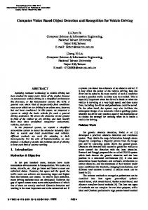
As mentioned before, our proposed method is to segment the wheel-soil image and then locate the wheelsoil boundary for sinkage measurement. Figure 2 illustrates the idea of sinkage measurement. Here, we show a diagram where the robot’s wheel sinks into the soil. The boundary is labeled in pink color. To determine the depth of wheel sinkage, we fit a Least-Squares Line (LSL) to the boundary. The wheel sinkage is estimated as Se=R-h, where R is the wheel’s radius and h is the distance between the wheel center and the LSL. Here, R is assumed to be constant, representing a rigid wheel. Fig. 2 Detection of wheel-sinkage However, known amounts of compression for pressurized or deformable wheels could be accounted for without difficulty. We use the NC method for image segmentation. A direct implementation of the NC method on the wheel-soil image is computationally expensive as the number of pixels (i.e., node number) is large. In [16] this problem is alleviated by down-sampling the input grey image to a reasonable size. However, the weight computation is still unaffordable. We resolve this computational bottleneck by: (1) partitioning the image into a number of homogeneous groups, called SuperPixels (SPs); (2) constructing a graph that takes each SP as a node; and (3) applying the NC method to the graph. The spatial location and color of each SP is computed as the centroid and mean color value of its image pixels. In our method, a node of graph G corresponds to a region rather than an image pixel. This substantially reduces the graph’s node number and thus the computational cost. The proposed method is described in the following subsections. A. Camera calibration We use a freely available camera calibration toolbox [17] to calibrate the camera. This calibration process removes the image distortion caused by the camera lens. B. Masking out unwanted regions We mask out the irrelevant image region (the inner part of the wheel rim) to save computational time. C. Obtaining Super-Pixels The resulting image is converted from RGB to L*u*v color space. In our current implementation, we use L*u*v color space due to its perceptual uniformity. The L*u*v image is then clustered into a number of SPs by the MeanShift (MS) algorithm [18]. D. Graph construction and partitioning We construct graph G (V , E ) by treating each SP as a node and calculate the similarities between nodes i and j as: ||F F || if Vi , V j are neighbors w(i, j ) e 0 otherwise 2 j 2
i
F
(4) where F(p) is the L*u*v color vector of node p; for p=i, j. SPi and SPj are considered as neighbors if they have more than one neighboring image pixel. Graph G is then partitioned into a predetermined number of segments, N, by the NC method. A prespecified segment number is not actually prescribed for the NC method; rather, the segmentation process stop when it finds N segments. The reason for doing so is that it is difficult to find an appropriate threshold for the re-cursive process, step 8 of the grouping algorithm, in Section II.B. E. Extraction of soil region and computation of wheel sinkage. The segments at the bottom of the image are grouped together to obtain the soil region. The edge image of this region gives the boundary of the soil and wheel. A LSL is fit to the pixels belonging to the boundary and h is then determined. As mentioned earlier, the depth of wheel sinkage is estimated as Se=R-h. In summary, our proposed wheel sinkage detection method is executed as follows: a) Acquire a wheel-soil image from the camera and undistort the image using the intrinsic parameters obtained from the camera calibration process. b) Mask-out the inner part of the wheel rim. c) Convert the resulting image to L*u*v space and apply the MS algorithm to obtain a number of SPs, denoted by Si; for i 1,, m . d) Construct a graph G on the SPs and compute the similarity matrix W of order m m by using (4). e) Apply the NC algorithm to graph G with W as the input to obtain N segments, ci for i=1,...,N, each of which contains a number of SPs. f) Extract the soil region by grouping the segments at the bottom part of the image. The edge image of the soil region, consisting of a set of pixels pi for i=1,…,k, gives the wheel-soil boundary. g) A LSL is fit to pi and the distance from the center of the wheel to the LSL, denoted by h, is computed. The depth of wheel sinkage is then given by Se=R-h.
4d shows the 135 SPs obtained after applying the MS algorithm to the image as shown in Fig. 4c. This causes a reduction of node number from 25600 to 135. As the edge number of a n-node graph is n(n-1)/2, the number of edge weight computations is reduced from 327667200 to 9045, about 3.6 10 4 times smaller. The amount of reduction in the number of edge weight computations will be referred to as Computation Reduction Factor (CRF) further on. The initial grouping of the SPs using the NC method is shown in Fig. 4e. It should be noted that the segmentation upon directly applying the NC method on the wheel-soil image (without using SPs) yields similar segmentation results but with a much larger computational cost. As the NC method considers both similarity in pixels’ intensity values and their spatial locations, it results in spatially coherent clusters. Since the bottom segments are in the soil region, we group them into one segment to obtain the soil region. The edge image of this region gives the wheel-soil boundary, which is shown in Fig. 4f. The boundaries extracted by using the OT and k-means methods are shown in Fig. 4g and Fig. 4h, respectively. We can observe that the OT method misclassifies some parts of the wheel as soil. This is because the dust-covered wheel has similar color as the soil and it is difficult to determine a good threshold to accurately partition the wheel and soil regions. The k-means clustering method results in many isolated clusters that make it difficult to extract the soil as a single contiguous region for
(a)
(b)
(c)
(d)
(e)
(f)
IV. EXPERIMENTAL RESULTS We have validated and compared our method with the OT and k-means methods in a number of representative situations. In all our experiments, we down sample the image from 640480 pixels to 160160 pixels after step b (Section III.E) for computational efficiency. A prespecified number of segments N=40 is used for graph partitioning using the NC method. For the results shown in this section, we represent an unlabeled segment in black and a labeled segment with a random non-black color. We represent the extracted wheel-soil boundary line in blue and the LSL by a dotted red line. The radius R of the robot wheel is 11 cm (and is assumed to be constant in experiments reported here). In the first experiment we test our method under normal illumination. Figure 4a and 4b shows the experimental setup and the wheel-soil image captured by the firewire camera, respectively. The image after masking out the inner part of the wheel rim is depicted in Fig. 4c. Figure
(g) (h) (i) Fig. 4 Extraction of wheel-soil boundary line under normal illumination, SPs = 135, CRF = 3.6104: (a) Actual scene; (b) Wheel image; (c) Wheel inner rim masked out from (b); (d) SPs of (c), (e) Results after applying the NC algorithm to (d); (f) Extracted soil boundary line; (g) Boundary extracted by the OT method; (h) Boundary extracted by the k-means method; (i) Extracted boundary of (f) and its LSL projected on the soilfree wheel image.
determining its boundary. Figure 4i depicts the soil boundary and its LSL projected onto the soil-free wheel image. We compute h as
described in step g (Section III.E). In this case h=5.69 cm, giving Se=5.31 cm. The true wheel sinkage St is found to be 5.50 cm. Hence, the sinkage measurement error is S=3.5%. The true sinkage is manually measured along a vertical line passing through the wheel’s center. The second experiment is conducted to test our method in very low illumination condition. We use a single source light with very low output to illuminate the environment (Fig. 5a). Figure 5b shows the captured wheel-soil image. The wheel-soil boundary extracted by our method is shown in Fig. 5c. As we can see, our method extracts the entire soil region as a single contiguous region and consequently the boundary line. The results of the OT and k-means methods are shown in Fig. 5d and Fig. 5e, where we observe the same problems of the two methods as mentioned in the first experiment. The projected boundary and the LSL are shown in Fig. 5f. The estimated wheel sinkage is Se=3.54 cm; the true wheel sinkage is St=4.0 cm; and the sinkage measurement error is S=-11.5%.
(a)
(b)
(c)
(d) (e) (f) Fig. 5 Extraction of wheel-soil boundary line under very low 4 illumination, SPs=106, CRF = 5.810 , Se=3.54 cm, St=4.0 cm, S=11.5%: (a) Actual scene; (b) Wheel image; (c) Boundary line extracted by our method; (d) Boundary extracted by the OT method; (e) Boundary extracted by the k-means method; (f) Extracted boundary and LSL projected on the soil-free wheel image.
The third experiment is carried out to test our method’s performance in the case of self-shadowing. Such conditions occur when a robot’s body part comes in between the light source and the wheel. We create this condition by placing the light source above the robot such that the shadow of the camera and its supporting arm is casted over the wheel. We show the scene in Fig. 6a. The casted shadow on the robot’s wheel can be seen in Fig. 6b. The extracted boundary using our method is shown in Fig. 6c. We can observe that our method is quite robust to selfshadows, whereas both the OT and k-means methods miss the shadow region as shown in Fig. 6d and Fig. 6e, respectively. The estimated wheel sinkage is Se=5.7 cm; the true wheel sinkage is St=5.5 cm; and the sinkage measurement error is S=3.6%. In the fourth experiment we validate our method under non-uniform illumination, i.e., part of the wheel is brighter than the other. Such conditions occur when a large object (e.g., an astronaut or another robot) casts a shadow on the wheel. To create this condition we place a piece of
cardboard such that it casts a shadow only on part of the wheel (Fig. 7a). The captured wheel-soil image is shown in Fig. 7b. The extracted boundary using our method is
(a)
(b)
(c)
(d) (e) (f) Fig. 6 Extraction of wheel-soil boundary line under low illumination, SPs=157, CRF=2.67104, Se=5.7cm, St=5.5cm, S=3.6%: (a) Actual scene; (b) Wheel image; (c) Boundary extracted using our method; (d) Boundary extracted by the OT method; (e) Boundary extracted by the kmeans method; (f) Extracted boundary and its LSL projected on the soilfree wheel image.
shown in Fig. 7c. The result of the OT method is shown in Fig. 7d. Here we can see that the darker area of the soil is not detected as soil region because their pixels’ intensity values are below the threshold value. Figure 7e shows the results of the k-means method where we can observe that the k-means method fails to detect the darker region and results in isolated clusters. Figure 7f shows the plot of the detected boundary and the LSL on the soil-free wheel image. For this experiment, the estimated wheel sinkage is Se=6.25 cm; the true wheel sinkage is St=5.5 cm; and the sinkage measurement error is S=13.6%.
(a)
(b)
(c)
(d) (e) (f) Fig. 7 Extraction of wheel-soil boundary line under non-uniform 4 illumination, SPs=146, CRF=3.110 , Se=6.25 cm, St=5.5 cm, S=13.6%: (a) Actual scene; (b) Wheel image; (c) Boundary extracted by our method; (d) Boundary extracted by the OT method; (e) Boundary extracted by the k-means method; (f) Extracted boundary and its LSL projected on the soil-free wheel image.
In each of our experiments, the robot is static and has only very small change in pose. It is reasonable to assume a constant wheel radius. It is noted that the LSL is a linear estimate of the wheel-soil boundary that is usually a curve. This might be the main contribution to the sinkage measurement error. In the future work, we will mark the
wheel-soil boundary manually and use its LSL to determine the true sinkage. This approach may result in more reasonable comparison between measured and true sinkage. We will also consider scenarios with deeper sinkage where the wheel-soil boundary goes over the lower inner part of the rim. Such a scenario can be detected by using the fitting error of the LSL. Then only the parts of the wheel-soil boundary that are on the tire will be used for sinkage measurement. Currently, the method is implemented in Matlab 7.7 on a computer with an AMD 2.60 GHz Phenom™ 9950 Quad-core Processor and 4 GB RAM. No parallel computation is performed in our current Matlab code. The operating system used is Window Vista Professional 64bit. It takes about 6 seconds to segment the images. We expect that it may achieve real-time performance if implemented in C++. Finally, it is worthwhile to mention that the camera’s suspension arm in a robot that is moving on rough terrain may cause vibration to the camera and deteriorate the image. This may result in sinkage measurement error. A solution to this problem is to use a miniature camera with a wider view angle. Since a 160160-pixel image is sufficient for sinkage measurement, we may use a small camera and reduce the mass on the arm. Also, we can reduce the arm’s length by using a smaller focal length (i.e., wider view angle) lens. This way, we will alleviate the motion-induce camera vibration. Two other issues that are worthy of further investigation are: First, the camera may have dual usesinkage detection and hazard avoidance. For instance, images for sinkage detection may be captured and processed every 1 meter of traverse and the other images can be used for hazard avoidance. Second, a method to keep the camera lens dust-free is essential for the application of the proposed method to lunar exploration tasks. V. CONCLUSIONS We have presented a new method that may reliably determine the wheel sinkage of a robot for lunar exploration missions. The method relies on identifying the wheel-soil boundary line which is the edge of the extracted soil region. We employ the Normalized Cuts (NC) method to segment the wheel-soil image and extract the soil region in its entirety. The nature of the graph partitioning methodutilizing both spatial distance and the color similarity between pixels in segmentationleads to a better segmentation performance of the proposed method. To determine the depth of wheel sinkage, we fit a least-square line to the pixels of the soil boundary. The wheel surface below this line represents the wheel sinkage. To reduce the computational cost of the graph partitioning process, we apply the MS method to preprocess the image into a number of SPs, from which a graph is constructed. We have tested our method in different scenarios, such as normal illumination, low lighting conditions, selfshadowing and non-uniform illumination. We find that our method is able to measure the wheel sinkage with good accuracy in all these conditions. We have also compared
the NC-based segmentation method with the OT and kmeans methods in our experiments and the results demonstrate that the NC-based segmentation method has a much better performance. The method may achieve realtime performance and it can be used for on-line wheel sinkage measurement by a lunar exploration robot. As a metal wheel is more distinctive from lunar regolith than a tire, the proposed method is expected to work well for a lunar robot with metal wheels. We also believe that the method can be adapted and used on a Mars rover where wheel sinkage is still a major problem to the rover’s mobility. REFERENCES [1] [2]
[3] [4] [5]
[6]
[7]
[8]
[9] [10] [11] [12] [13] [14]
[15]
[16] [17] [18]
M. G. Bekker, “Off-road locomotion,” the University of Michigan Press, Ann Arbor, MI, 1960. K. Iagnemma, S. Kang, H. Shibly, and S. Dubowsky, “Online terrain parameter estimation for wheeled mobile robots with application to planetary rovers,” IEEE Transactions on Robotics, vol. 20, no. 2, pp. 921-927, 2004. C. A. Brooks, K. D. Iagnemma, S. Dubowsky, “Visual wheel sinkage measurement for planetary rover mobility characterization,” Autonomous Robots, v.21, no.1, pp.55-64, 2006. G. Reina, L. Ojeda, A. Milella, and J. Borenstein, “Wheel slippage and sinkage detection for planetary rovers,” IEEE/ASME Transactions on Mechatronics, vol. 11, no. 2, pp. 185-195. L. Ojeda, D. Cruz, G. Reina, and J. Borenstein, “Current-based slippage detection and odometry correction for mobile robots and planetary rovers,” IEEE Transactions on Robotics, vol. 22, no. 2, pp. 366-378, 2006. K. Yoshida, T. Watanabe, N. Mizuno and G. Ishigami, “Slip, traction control, and navigation of a lunar rover,” in Proc. 7th International Symposium on Artificial Intelligence, Robotics, and Automation in Space, Nara, Japan, May 2003. K. Iizuka, Y. Kunii, Y. Kuroda and T. Kubota, “Design scheme on Wheeled Forms of Exploration Rover in consideration of Mechanism between Wheels and Soil,” in Proc. 9th International Symposium on Artificial Intelligence, Robotics, and Automation in Space, Los Angeles, CA, Feb. 2008. D. Wettergreen, D. Jonak, D. Kohanbash, et al., “Design and experimentation of a rover concept for lunar crater resource survey,” in Proc. 47th AIAA Aerospace Sciences Meeting Including The New Horizons Forum and Aerospace Exposition, Orlando, FL, Jan. 2009. L. Ding, H.-B. Gao, Z.-Q. Deng and J.-G. Tao, “Wheel slip-sinkage and its prediction model of lunar rover,” Journal of Central South University of Technology, vol. 17, pp. 129-135, 2010. N. Otsu, “A threshold selection method from gray-level histograms,” IEEE Transactions on Systems, Man, and Cybernetics, vol. 9, no. 1, pp. 62-66, 1979. J. B. MacQueen, “Some methods for classification and analysis of multivariate observations,” University of California Press, Berkeley, CA, 1967. J. Malik, S. Belongie, J. Shi, and T. Leung, “Textons, contours and regions: cue combination in image segmentation,” in Proc. International Conference on Computer Vision, 1999, pp. 918-925. J. Shi and J. Malik, “Normalized cuts and image segmentation,” IEEE Transactions on Pattern Analysis and Machine Intelligence, vol. 22, no. 8, pp. 888-905, 2000. S. Sarkar and P. Soundararajan, “Supervised learning of large perceptual organization: Graph spectral partitioning and learning automata,” IEEE Transactions on Pattern Analysis and Machine Intelligence, vol. 22, no. 5, pp. 504–525, 2000. Z.-Y.Wu and R. Leahy, “An optimal graph theoretic approach to data clustering: Theory and its application to image segmentation,” IEEE Transactions on Pattern Analysis and Machine Intelligence., vol. 15, no. 11, pp. 1101–1113, 1993. http://www.cis.upenn.edu/~jshi/software/: A matlab library for Normalized Cuts based image segmentation. http://www.vision.caltech.edu/bouguetj/calib_doc/ W. Tao, H. Jin, and Y. Zhang, “Color image segmentation based on mean shift and normalized cuts,” IEEE Transactions on Systems, Man, and Cybernetics, part B, vol. 37, no. 5, pp. 1382-1389, 2007.