Computing Integrals over Polynomially Defined Regions and Their ...

Computing Integrals over Polynomially Defined Regions and Their Boundaries in 2 and 3 Dimensions Michael J. Wester Department of Mathematics and Statistics Center for High Performance Computing University of New Mexico Albuquerque NM 87131-1141 USA Yuzita Yaacob Department of Industrial Computing National University of Malaysia 43100 Malaysia Stanly Steinberg Department of Mathematics and Statistics Cancer Research and Treatment Center University of New Mexico Albuquerque NM 87131-1141 USA June 2, 2011 Key Words: area integral, line integral, volume integral, surface integral, iterated integrals, cylindrical algebraic decomposition Short title: Two and Three Dimensional Integrals

1

Contents 1 Introduction

4

2 Integrals

5

3 Regions and Volumes

7

4 Two Dimensional Examples 11 4.1 Simple Examples . . . . . . . . . . . . . . . . . . . . . . . . . 12 5 Boxes and Planar Integrals 5.1 Examples . . . . . . . . . . 5.2 Boundaries of Boxes . . . . 5.3 Boundaries of Regions . . . 5.4 Integrals Over Boundaries of 5.5 Examples Continued . . . . 5.6 Green’s Theorem . . . . . .

. . . . . . . . . . . . . . . . . . Boxes and . . . . . . . . . . . .

. . . . . . . . . . . . . . . Regions . . . . . . . . . .

6 Advanced Two-Dimensional Examples 6.1 A Hexagon . . . . . . . . . . . . . . . . . 6.2 The Intersection of Two Circles . . . . . 6.3 A Self Intersecting Curve . . . . . . . . . 6.4 The Intersection of Two Ellipses . . . . . 6.5 Examples with Symbolic Parameters . . 6.5.1 A Circle with Parametric Radius 6.5.2 The Witch of Agnesi . . . . . . . 7 Three-Dimensional Integration 7.1 3D Cylinders . . . . . . . . . . . . 7.2 The Boundary of a Cylinder . . . . 7.3 The Divergence Theorem . . . . . . 7.4 General Curves and Surfaces in 3D

. . . .

. . . .

. . . .

. . . . . . . . . . .

. . . . . . . . . . .

. . . . . . . . . . .

. . . . . . . . . . .

. . . . . . . . . . . . . . . . .

. . . . . . . . . . . . . . . . .

. . . . . . . . . . . . . . . . .

. . . . . . . . . . . . . . . . .

. . . . . . . . . . . . . . . . .

. . . . . . . . . . . . . . . . .

. . . . . . . . . . . . . . . . .

. . . . . .

14 14 15 17 19 20 21

. . . . . . .

22 22 24 25 26 27 27 28

. . . .

28 29 30 31 31

8 Summary

32

A Parameterization of Boundary Curves

36

2

List of Figures 1 2 3 4 5 6 7 8 9 10 11

An Annulus . . . . . . . . . . . . . . . . . . . . . . . . . . . A Diamond . . . . . . . . . . . . . . . . . . . . . . . . . . . An Unbounded Region . . . . . . . . . . . . . . . . . . . . . A Generalized Box (Cylinder). . . . . . . . . . . . . . . . . . The Boxes for a Circle and Square and Their Complements. Tangents and Normals for a Box. . . . . . . . . . . . . . . . A Hexagon. . . . . . . . . . . . . . . . . . . . . . . . . . . . The Intersection of Two Circles. . . . . . . . . . . . . . . . . A self Intersecting Curve. . . . . . . . . . . . . . . . . . . . . The Intersection of Two Ellipses. . . . . . . . . . . . . . . . The Intersection of a Circular Cylinder and a Sphere. . . . Abstract We use the cylindrical algebraic decomposition algorithms implemented in Mathematica to produce procedures to analytically compute integrals over polynomially defined regions and their boundaries in two and three dimensions. Using these results, we can implement the Divergence Theorem in three dimensions or the Green’s theorems in two dimensions. These theorems are of central importance in the applications of multidimensional integration. They also provide a strong correctness test for the implementation of our results in a computer algebra system. The resulting software can solve many of the two and some of the three dimensional integration problems in vector calculus textbooks. The three dimensional results are being extended. The results in this paper are being included in an automated student assistant for vector calculus.

3

. . . . . . . . . . .

7 8 9 11 12 16 22 24 25 27 29

1

Introduction

The evaluation of integrals over planar regions and curves in two dimensions is a problem addressed in most (probably all) introductory one-year calculus textbooks. More advanced texts will also discuss integrals over volumes, surfaces and curves in three dimensions [5]. These topics are central to the application of vectors in science and engineering. If the geometry or the function being integrated is complicated, then the method of choice for evaluation is numerical. Here, we focus on developing procedures for the analytic evaluation of such integrals when the ingredients in the integral are sufficiently simple. In two dimensions, we focus on planar regions and curves that are the boundaries of such regions. In three dimensions, we only consider simple volumes and the surfaces that are boundaries of these regions. We assume that the planar regions and volumes can be described using polynomial inequalities. An important contribution is the extension of the integration tools in Mathematica to boundary curves and surfaces, allowing the use of Green’s and the Divergence Theorems, a central part of integration theory in vector calculus. The basic tool in our work is the cylindrical algebraic decomposition (CAD) algorithm that can decompose complicated regions into a union of simple regions [1, 2]. This algorithm requires the region to be described by polynomial inequalities. Historically, the CAD algorithm was used to solve quantifier elimination problems [3, 4]. For applications of quantifier elimination algorithms to engineering problems, see [8, 10]. For newer types of CAD algorithms, see [6]. Our ultimate goal is to include the material in this paper into a program that helps students learn vector calculus [13, 14]. This program uses Mathematica, so we have implemented our ideas in this system. Mathematica can already evaluate area and volume integrals using procedures based on [11, 12]. However, for the student assistant, we need to know some of the intermediate results, so these tools are not exactly what we need. More importantly, these tools cannot find integrals over the boundaries of regions. Consequently, we will return to the ideas presented in [9, 11] to build our vector calculus tools.

4

2

Integrals

If R is a region and C is a curve in a two dimensional plane, then mathematicians write the integrals that we will study as Z ZZ Z Z ds f= f (x, y) dx dy , g = g(ξ) dξ . (2.1) dξ R R C where x and y are real variables, f is a real valued function defined on the region, g is a real valued function of a real variable, s is an arc length variable on the curve and ξ is a parameter. Also, if Ω is a volume and S is a surface in three dimensional space, then we will study integrals of the form Z ZZZ Z ZZ f= f (x, y, z) dx dy dz , h= h(ξ, η) J(x, y, z; ξ, η) dξ dη . Ω

Ω

S

(2.2) where x, y and z are real variables, f is a real valued function defined in the volume, h is a real valued function of two real variables, J is a surface area element, and ξ and η are parameters. We will focus on curves that are the boundary of a region, C = ∂R, and surfaces that are boundaries of volumes, S = ∂Ω. Integrals over planar regions will be reduced to a sum of iterated integrals, while integrals over curves will be reduced to a sum of integrals over intervals. In three dimensions, integrals over volumes will be reduced to a sum of triple integrated integrals, integrals over surfaces to a sum of double iterated integrals. Many computer algebra systems can evaluate the resulting integrals if this is mathematically possible. We write the integrals as sums of simpler integrals by writing the region or volume as a union of simple regions or volumes where integrals over each part can be written as an iterated integral or an integral over an interval. To accomplish our goals, we use some basic facts about integrals. The first is that integrals over lower dimensional sets are zero. For volume integrals, adding or removing surfaces, curves or points from the volume doesn’t change the value of the integral. For integrals over regions in the plane or surfaces in three dimensions, adding or removing curves and points does not affect the value of the integrals. Finally, for curves, adding or removing points doesn’t change the value. For applications that involve Green’s or the Divergence Theorems, it is customary to assume the regions are non-trivial and contain their boundary. 5

More formally, we assume that the region satisfies clo int R = R , where clo means the closure and int means the interior of the set. It is also important that the boundary consists of a finite number of smooth pieces. Another crucial fact is that if R is the union of essentially disjoint sets, that is, if K is a positive integer and R = ∪K k=1 Sk ,

(2.3)

where int Sj ∧ int Sk = ∅ ,

1 ≤ j, k ≤ K ,

and ∅ is the empty set, then Z

f=

R

K Z X k=1

f.

Sk

The situation for boundary integrals is more complex because boundaries are oriented. If Sj and Sk have a portion of their boundaries in common, then the orientation of these parts must be opposing, and thus they are not part of the boundary of R and so can be eliminated from the boundary calculation. With this understanding, ∂R = ∪K k=1 ∂Sk . This operation is also commonly written as a sum rather than a union to indicate that the parts with opposite orientation cancel. This simplification gives ∂R = ∪Jj=1 Cj , where J is a positive integer, Cj is an oriented curve and the Cj are essentially disjoint. Then Z J Z X g= g. ∂R

j=1

Cj

For some important boundary integrals, the simplification is not required, but it does reduce the amount of computation needed to find the integral.

6

y 3

2

1

x -3

-2

1

-1

2

3

-1

-2

-3

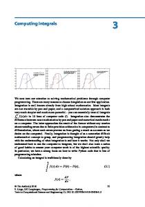
Figure 1: An Annulus

3

Regions and Volumes

We will assume that the regions and volumes can be described by a finite number of polynomials. This well cover many problems from vector calculus, but not regions that are described by logarithms, exponentials, trigonometric, or more general functions. More precisely, we will assume that our sets are semi-algebraic, that is, a region R is defined by R = {(x, y) : F (x, y) is true } , where F (x, y) is a finite logical formula that involves only real polynomials in the real variables x and y. We will assume that a volume Ω is defined by Ω = {(x, y, z) : F (x, y, z) is true } , where F (x, y, z) is a finite logical formula that involves only real polynomials in the real variables x, y and z. The logical formulas can use any of ≤, ≥, and = to connect two polynomials and not (¬), and (∧), and or (∨) in the construction of the logical formulas. For example, x2 + y 2 ≥ 1 ∧ x2 + y 2 ≤ 2 defines the annulus shown in Figure 1. A basic theorem in logic says that we can write any formula as the ∨ of a finite number of terms that are an ∧ of a finite number of terms, that is, the set is a union of intersections of sets where each set is given by a polynomial equality or inequality. 7

Figure 2: A Diamond The powerful cylindrical algebraic decomposition (CAD) algorithm [3, 4] decomposes general semi-algebraic sets into unions of simpler sets that are called cylinders in the computational algebraic geometry literature. However, we are not interested in general semi-algebraic sets, but only sets that are the closure of their interior. Mathematica provides two CAD functions: CylindricalDecomposition, which we abbreviate CD; GenericCylindricalDecomposition, which we abbreviate GCD. Neither of these do exactly what we want, as the following two examples illustrate. Consider the region D defined by the formula D(x, y) = x + y ≥ −1 ∧ x − y ≥ −1 ∧ x − y ≤ 1 ∧ x + y ≤ 1 ,

(3.1)

which describes a closed set that is the diamond in Figure 2. The integral of a function f over this region is Z 0 Z x+1 Z 1 Z −x+1 f (x, y) dy dx + f (x, y) dy dx . (3.2) −1

0

−x−1

x−1

If we apply CD to the formula (3.1) for D, we get (x = −1 ∧ y = 0) ∨ (−1 < x ≤ 0 ∧ −x − 1 ≤ y ≤ x + 1) ∨ (0 < x < 1 ∧ x − 1 ≤ y ≤ 1 − x) ∨ (x = 1 ∧ y = 0) ,

(3.3)

which lists two of the corner points as separate cylinders. We can eliminate the terms containing = as planar integrals over points are zero. Note that 8

Figure 3: An Unbounded Region the vertical line segment that is part of x = 0 is listed as part of one of the triangles, but not the other. If we apply the rules ≥→> and ≤→< to the formula (3.1) for D and then apply CD to the result, we get (−1 < x ≤ 0 ∧ −x − 1 < y < x + 1) ∨ (0 < x < 1 ∧ x − 1 < y < 1 − x) , which is what we got by eliminating the equalities from (3.3). Alternatively, if we apply GCD and then take the the first part of the answer, we get (−1 < x < 0 ∧ −x − 1 < y < x + 1) ∨ (0 < x < 1 ∧ x − 1 < y < 1 − x) . This is a subset of the interior of D with the property that its closure is again D. Any of these results can easily translated into the integrals in (3.2), but we prefer this last form because of its symmetry, that is, no part of x = 0 is included in the answer. Cylinders for unbounded regions have a different algebraic form than those for bounded regions. Integrals over such regions are called improper. Consider the closed unbounded region xy ≤ 1 ∧ x ≥ 0 ∧ y ≥ 0 shown in Figure 3. From CD, we get   1 (x = 0 ∧ y ≥ 0) ∨ x > 0 ∧ 0 ≤ y ≤ , x 9

(3.4)

while from the other two methods we get x> 0∧0 1 .

It’s closure is given by

F (x, y) = x2 + y 2 ≥ 1 . The complement of the square is more interesting. It is an open set described by the formula ¬(x ≥ −1 ∧ x ≤ 1 ∧ y ≥ −1 ∧ y ≤ 1) , which can be expanded to x < −1 ∨ x > 1 ∨ y < −1 ∨ y > 1 . The formula for the closure of this region is: F (x, y) = x ≤ −1 ∨ x ≥ 1 ∨ y ≤ −1 ∨ y ≥ 1 . The closed boxes for the complement of the disk are B1 (x, y) B2 (x, y) B3 (x, y) B4 (x, y)

= −∞ < x ≤ −1 = −1 ≤ x ≤ 1 = −1 ≤ x ≤ 1 = 1≤x 0 is given by  R = (x, y) : x2 + y 2 ≤ a2 . 27

Find the area of this circle. The CAD for this region, using the variables a, x, y, is a single box √ √ a > 0 ∧ −a ≤ x ≤ a ∧ − a2 − x2 ≤ y ≤ a2 − x2 .

If we eliminate the first term, then this is in the correct form for our boxes. The area is given by Z a Z √a2 −x2 dy dx . √ −a

− a2 −x2

Mathematica can easily evaluate this integral to get π a2 . 6.5.2

The Witch of Agnesi

The Witch of Agnesi is a curve given by 8 a3 , −∞ < x < ∞ . x2 + 4 a2 Find the area between this curve and the x-axis. The region is given by  R = (x, y) : y ≥ 0 ∧ y (x2 + 4 a2 ) ≤ 8 a3 ∧ a > 0 . y=

The CAD for this region, using the variables a, x, y, is the infinite box

8a3 . 4a2 + x2 If we remove the first term and note that x missing, then we get a box in standard form: 8a3 −∞ < x < ∞ ∧ 0 ≤ y ≤ 2 . 4a + x2 This is easily converted into an area integral that Mathematica can evaluate, yielding 4 πa2 . a>0∧0≤y ≤

7

Three-Dimensional Integration

In this section, we will discuss integrals over generic three-dimensional cylinders, but not regions, because we have not implemented how to convert cylinders with a non-standard descriptions to a uniform description and we have not worked out all of the needed boundary simplification rules. For volumes, the ideas for planar cylinders apply to three dimensional cylinders with only straightforward changes. Computing the boundary of a cylinder is more complex. 28

2 1 0 -1 -2 2

1

0

-1

-2 -2 -1 0 1 2

Figure 11: The Intersection of a Circular Cylinder and a Sphere.

7.1

3D Cylinders

A 3D cylinder has the form a ≤ x ≤ b ∧ c(x) ≤ y ≤ d(x) ∧ g(x, y) ≤ z ≤ h(x, y) ,

(7.1)

where a and b are real constants, c and d are real valued functions of a single real variable, and g and h are real valued function of two variables. The integral of f = f (x, y, z) over the cylinder (7.1) is Z b Z d(x) Z h(x,y) f (x, y, z) dz dy dx . a

c(x)

g(x,y)

As in two dimensions, this can now be used with the CAD algorithm to reduce integrals over three dimensional regions to iterated integrals. A simple example is given by a circular cylinder cut out of a sphere, x2 + y 2 + z 2 ≤ 4 ∧ x2 + y 2 ≤ 1 , shown in Figure 11. The integral of f over the region is given by Z √ Z Z √ 1

1−x2

−1

√ − 1−x2

4−x2 −y 2

−

√

4−x2 −y 2

29

f (x, y, z) dz dy dx .

(7.2)

Mathematica √
can be used to compute that the volume of the region is 8 4π 3 − 3 .

7.2

The Boundary of a Cylinder

The boundary of the cylinder (7.1) is given by {x, y} , a ≤ x ≤ b , c(x) ≤ y ≤ d(x) , {x, y} , a ≤ x ≤ b , c(x) ≤ y ≤ d(x) , {x, z} , a ≤ x ≤ b , {x, z} , a ≤ x ≤ b , {y, z} , {y, z} ,

x = b, x = a,

z = g(x, y) , z = h(x, y) ,

~1 +N ~2 −N

~3 g(x, c(x)) ≤ z ≤ h(x, c(x)) , +N ~4 g(x, d(x)) ≤ z ≤ h(x, d(x)) , −N

y = c(x) , y = d(x) , c(x) ≤ y ≤ d(x) , c(x) ≤ y ≤ d(x) ,

g(x, y) ≤ z ≤ h(x, y) , g(x, y) ≤ z ≤ h(x, y) ,

~5 +N ~6 −N

where   ~ 1 = g (1,0) (x, y), g (0,1) (x, y), −1 , N ~ 2 = h(1,0) (x, y), h(0,1) (x, y), −1 , N ~ 3 = {c′ (x), −1, 0} , ~ 4 = {d′ (x), −1, 0} , N N ~ 5 = {1, 0, 0} . ~ 6 = {1, 0, 0} . N N and the superscripts indicate derivatives. Each piece of the boundary contains 5 entries. The first entry is the two variables used to parameterize the piece. The next 3 entries give the equation for the piece and the limits on the variables. The final entry is an outward normal to the piece. The surface integral of the normal component of V~ is R b R d(x) ~ 1 (x, y) · V ~ (x, y, g(x, y)) dy dx N a c(x) R b R d(x) ~ 2 (x, y) · V~ (x, y, h(x, y)) dy dx − a c(x) N R b R h(x,c(x)) ~ 3 (x) · V ~ (x, c(x), z) dz dx + a g(x,c(x)) N R b R h(x,d(x)) ~ 4 (x) · V ~ (x, d(x), z) dz dx − a g(x,d(x)) N R d(b) R h(b,y) ~5 · V ~ (b, y, z) dz dy + c(b) g(b,y) N R d(a) R h(a,y) ~ 6 · V~ (a, y, z) dz dy − c(a) g(a,y) N The integral of the normal component of a vector field over the boundary of the circular cylinder intersected with a sphere (7.2) is too lengthy to print 30

here, but the formula is given in a notebook. We can compute the area of ~ ·V ~ with the square root of N ~ ·N ~ in the previthe surface by replacing N ous formulas. The surface area of the intersection of the √ circular cylinder intersected with the sphere shown in Figure 11 is 4 (4 − 3)π.

7.3

The Divergence Theorem

The divergence theorem is Z

Ω

~ · V~ = ∇

Z

∂Ω

~, V~ · N

~ = (∂/∂x , ∂/∂y , ∂/∂z) is the where Ω is simply connected 3D region, ∇ ~ divergence operator, V~ is a vector field, ∂Ω is the boundary of Ω, and N ~ is the outward normal to the surface. If we choose V = (x/3, y/3, z/3), ~ ·V ~ = 1 and consequently the surface integral gives the volume of the then ∇ region. This fact was used to to check our surface integration formulas.

7.4

General Curves and Surfaces in 3D

In 3D, algebraic surfaces are be given by P (x, y, z) = 0, while algebraic curves are given by P (x, y, z) = 0 ∧ Q(x, y, z) = 0. However simple this seems, there are several problems. First, the objects can be degenerate. For example, if P (x, y, z) = x2 + y 2 + z 2 + 1, then the surface will be the empty set. If P can be factorized, then the zero set can be the union of two or more simpler curves. Another problem is that such curves and surfaces have two possible orientations and we do not see a nice way to specify their orientation. If the curve or surface is given parametrically, which is the case in many applications, then an orientation is induced by the parameterization. If a curve C is oriented and starts at a point P1 and ends at the point P2 and f is a smooth function, then the Potential Theorem (Fundamental Theorem of Calculus) can be applied: Z ~ = f (P2 ) − f (P1 ) . ∇f C

~ the right-hand rule In the case of an oriented surface S with normal N, ~ ~ is a smooth vector orients the boundary ∂S with a tangent vector T . If V 31

field, then one can apply Stokes’ Theorem, Z Z ~ ~ ~ ~ · T~ , ∇×V ·N = V S

∂S

to evaluate integrals. Some examples are given in a notebook.

8

Summary

We have shown that combining the Mathematica cylindrical algebraic decomposition (CAD) routines with some computer algebra tools that we developed that put the CADs into a standard form allows us to break up complex two dimensional regions into cylinders and then reduce integrals over the regions to sums of iterated integrals. If the iterated integrals are not too complicated, they can be evaluated analytically by most computer algebra systems. In the two dimensional case, we can also find the length of the boundary curve of the region and two types of boundary integrals. We can also use the two dimensional versions of the Divergence and Stokes’ Theorems to evaluate integrals and check our codes. Our 3D results only apply to regions that are cylinders. We can find the volume and the area of the surface area of the cylinder. In 3D, there is only one integration theorem for volumes and their boundaries: the divergence theorem. We use the divergence theorem to check our surface and volume integral formulas. Extending these results to more general regions is in progress. Importantly, the computation of the length of a curve and the area of a surface rely on a “boundary simplification” algorithm. We have implemented a general simplification heuristic in two dimensions and a partial heuristic in three dimensions. It is an important problem to convert these heuristics to algorithms that are proven correct. It is also important that we do not use the full power of the CAD algorithm. Because integrals over “small” sets are zero, we can restrict our attention to regions that are closures of their interiors. A CAD restricted to such sets should be much faster and produce more appropriate answers than the general CAD. We have also included some simple examples where the description of the integration region contains a parameter. Here, the CAD is applied simultaneously to the integration variables and the parameter.

32

We have implemented some ideas for general curves and surfaces—surfaces that are not boundaries of regions—in 3D. Extending these results and implementing Stokes’ Theorem is also in progress. The algebraic methods developed here can be used as a basis for numerically estimating the volume of a region in a multi-dimensional space [7]. It should also be possible to extend our results to regions defined by simple transcendental functions.

33

References [1] D. S. Arnon, G. E. Collins, and S. McCallum. Cylindrical algebraic decomposition I: The basic algorithm. SIAM Journal on Computing, 13(4):865–877, 1984. [2] C. W. Brown. Simple CAD construction and its applications. J. Symbolic Comput., 31:521–547, 2001. [3] B. F. Caviness and J. R. Johnson, editors. Quantifier Elimination and Cylindrical Algebraic Decomposition, Texts and Monographs in Symbolic Computation, New York, 1998. Springer-Verlag. [4] G.E. Collins and H.Hong. Partial cylindrical algebraic decomposition for quantifier elimination. Journal of Symbolic Computation, 12(3):299–328, Sep 1991. [5] H. F. Davis and A. D. Snider. Introduction to Vector Analysis. William C Brown Pub., 1995. [6] Andreas Dolzmann and Volker Weispfenning. Local quantifier elimination. In ISSAC ’00: Proceedings of the 2000 international symposium on Symbolic and algebraic computation, pages 86–94, New York, NY, USA, 2000. ACM. [7] D. Henrion, J. B. Lasserre, and C. Savorgnan. Approximate volume and integration for basic semialgebraic sets. SIAM Rev., 51(4):722–743, 2009. [8] Hoon Hong, Richard Liska, and Stanly Steinberg. Testing stability by quantifier elimination. J. Symb. Comput., 24(2):161–187, 1997. [9] S. McCallum. Solving polynomial strict inequalities using cylindrical algebraic decomposition. Comput. J., 36:432–438, 1993. [10] Hiroyuki Sawada and Xiu-Tian Yan. Application of Gr¨obner bases and quantifier elimination for insightful engineering design. Math. Comput. Simul., 67(1-2):135–148, 2004. [11] Adam Strzebo´ nski. Solving systems of strict polynomial inequalities. J. Symb. Comput., 29(3):471–480, 2000. 34

[12] Adam Strzebo´ nski. Applications of algorithms for solving equations and inequalities in mathematica. In A. Seidl A. Dolzmann and T. Sturm, editors, Proceedings of the A3L 2005, pages 243–248, Passau, Germany, 2005. Conference in Honor of the 60th Birthday of Volker Weispfenning. [13] Yuzita Yaacob. Interactive Learning—Mathematica Enhanced Vector calculus (ILMEV). PhD thesis, International Islamic University Malaysia, Gombak, Selangor Darul Ehsan, Malaysia, 2007. [14] Yuzita Yaacob, Michael Wester, and Stanly Steinberg. ILMEV: An automated learning assistant for vector calculus. submitted, 2009.

35

A

Parameterization of Boundary Curves

Here we justify the formulas used in (5.6) by using a standard parameterization that moves points in a counter clockwise direction on the boundary curve: C1 C2 C3 C4

: : : :

x1 (ξ) x2 (ξ) x3 (ξ) x4 (ξ)

= = = =

a + (b − a)ξ , b, b + (a − b)ξ , a,

y1 (ξ) y2 (ξ) y3 (ξ) y4 (ξ)

= = = =

l(a + (b − a)ξ) , l(b) + (u(b) − l(b))ξ , u(b + (a − b)ξ) , u(a) + (l(a) − u(a))ξ .

where a and b are finite and 0 ≤ ξ ≤ 1. If a or b are infinite, then a special parameterization is needed. The work and flux integrals are given by Z 1 Z 1 ~ ~ ~ (x(ξ), y(ξ))·N(x(ξ), ~ W = V (x(ξ), y(ξ))·T (x(ξ), y(ξ)) dξ , F = V y(ξ)) dξ . 0

0

For curves 1 and 3, we make a change of variables from ξ to x, while for curves 2 and 4, we change from ξ to y. The work and flux integrals transform in the same manner, so for simplicity we will only transform the work integrals. For the first curve, ξ = (x−a)/(b−a), dξ = dx/(b−a), x(0) = a, x(1) = b and T~1 = (x′ (ξ), y ′(ξ)) = (b − a, l′ (x)(b − a)) = (b − a)(1, l′ (x)) . Consequently, W =

Z

a

b

~ (x, l(x)) · (1, l′ (x)) dx . V

For the third curve, ξ = (x − b)/(a − b), dξ = dx/(a − b), x(0) = b, x(1) = a and T~3 = (x′ (ξ), y ′(ξ)) = (a − b, u′ (x)(a − b)) = (a − b)(1, u′ (x)) . Consequently, Z a Z b ′ ~ (x, u(x)) · (−1, −u′ (x)) dx . W = V~ (x, u(x)) · (1, u (x)) dx = V b

a

For the second curve, ξ = (y − l(b))/(u(b) − l(b)), dξ = dy/((u(b) − l(b)), y(0) = l(b), y(1) = u(b), and T~2 = (x′ (ξ), y ′(ξ)) = (0, u(b) − l(b)) = (u(b) − l(b))(0, 1) . 36

Consequently, W =

Z

u(b)

l(b)

V~ (b, y) · (0, 1) dy .

For the fourth curve, ξ = (y − u(a))/(l(a) − u(a)), dξ = dy/((l(a) − u(a)), y(0) = u(a), y(1) = l(a), and T~4 = (x′ (ξ), y ′(ξ)) = (0, l(a) − u(a)) = (l(a) − u(a))(0, 1) . Consequently, W =

Z

l(a)

u(a)

V~ (a, y) · (0, 1) dy =

37

Z

u(a)

l(a)

~ (a, y) · (0, −1) dy . V