Communicated by Richard Andersen. Computing Optical Flow in the Primate .... H. Taichi Wang, Bimal Mathur, Christof Koch. 1985). We also require a set of n ...
Communicated by Richard Andersen
Computing Optical Flow in the Primate Visual System H. Taichi Wang Bimal Mathur Science Center, Rockwell International, Thousand Oaks, CA 91360, USA
Christof Koch Computation and Neural Systems Program, Divisions of Biology and Engineering and Applied Sciences, 216-76, California Institute of Technology, Pasadena, CA 91125, USA
Computing motion on the basis of the time-varying image intensity is a difficult problem for both artificial and biological vision systems. We show how gradient models, a well known class of motion algorithms, can be implemented within the magnocellular pathway of the primate’s visual system. Our cooperative algorithm computes optical flow in two steps. In the first stage, assumed to be located in primary visual cortex, local motion is measured while spatial integration occurs in the second stage, assumed to be located in the middle temporal area (MT). The final optical flow is extracted in this second stage using population coding, such that the velocity is represented by the vector sum of neurons coding for motion in different directions. Our theory, relating the single-cell to the perceptual level, accounts for a number of psychophysical and electrophysiological observations and illusions. 1 Introduction
In recent years, a number of theories have been advanced at both the computational and the psychophysical level, explaining aspects of biological motion perception (for a review see Ullman 1981; Nakayama 1985; Hildreth and Koch 1987). One class of motion algorithms exploit the relation between the spatial and the temporal intensity change at a particular point (Fenneman and Thompson 1979; Horn and Schunck 1981; Marr and Ullman 1981; Hildreth 1984). In this article we address in detail how these algorithms can be mapped onto neurons in striate and extrastriate primate cortex (Ballard et al. 1983). Our neuronal implementation is derived from the most common version of the gradient algorithm, proposed within the framework of machine vision (Horn and Schunck 1981). Due to the ”aperture” problem inherent in their definition of optical flow, only the component of Neural Cornputation 1, 92-103 (1989) @ 1989 Massachusetts Institute of Technology
Computing Optical Flow in the Primate Visual System
93
motion along the local spatial brightness gradient can be recovered. In their formulation, optical flow is then computed by minimizing a twopart quadratic variational functional. The first term forces the final optical flow to be compatible with the locally measured motion component ("constraint line term"), while the second term imposes the constraint that the final flow field should be as smooth as possible. Such as "smoothness" or "continuity" constraint is common to most early vision algorithms. 2 A Neural Network Implementation
Commensurate with this method, and in agreement with psychophysical results (e.g. Welch 19891, our network extracts the optical flow in two stages (Fig. 1). In a preliminary stage, the time-varying image Z ( i , j ) is projected onto the retina and relayed to cortex via two neuronal pathways providing information as to the spatial location of image features ( S neurons) and temporal changes in these features (T neurons): S ( i , j ) = V 2 G * I ( i , j and ) T ( i , j )= a ( V * G * I ( i ,j) ) /&where , * is the convolution operator and G the 2-D Gaussian filter (Enroth-Cugell and Robson 1966; Marr and Hildreth 1980; Marr and Ullman 1981). In the first processing stage, the local motion information is represented using a set of n ON-OFF orientation- and direction-selective cells U , each with preferred direction indicated by the unit vector o k :
where t is a constant and Vk is the spatial derivative along the direction Ok. This derivative is approximated by projecting the convolved image S ( i , j ) onto a "simple" type receptive field, consisting of a 1 by 7 pixel positive (ON) subfield adjacent to a 1 by 7 pixel negative (OFF) subfield. The cell U responds optimally if a bar or grating oriented at right angles to Ok moves in direction Ok.Note that U is proportional to the product of a transient cell ( T )with a sustained simple cell with an odd-symmetric receptive field, with an output proportional to the magnitude of local component velocity (as long as \V&'(z,j)l > t). At each location i , j , n such neurons code for motion in n directions. Equation (2.1) differs from the standard gradient model in which U = - T / V k S , by including a gain control term, t, such that U does not diverge if the stimulus contrast decreases to zero. t is set to a fixed fraction of the square of the maximal magnitude of the gradient V S for all values of z,j. Our gradient-like scheme can be approximated for small enough values of the local contrast (i.e. if lVS(i,j)12< e), by -T(z,j)VkS(z,j). Under this condition, our model can be considered a second-order model, similar to the correlation or spatio-temporal energy models (Hassenstein and Reichardt 1956; Poggio and Reichardt 1973; Adelson and Bergen 1985; Watson and Ahumada
94
H. Taichi Wang, Bimal Mathur, Christof Koch
1985). We also require a set of n ON-OFF orientation- but not directionselective neurons E , with E ( i , j ,k ) = IVkS(i,j ) ] ,where the absolute value ensures that these neurons only respond to the magnitude of the spatial gradient, but not to its sign. We assume that the final optical flow field is computed in a second stage, using a population coding scheme such that the velocity is represented within a set of n‘ neurons V at location i , j , each with preferred direction Ok with V(i, j) = ETLl V ( i ,j , k)@k. Note that the response of any individual cell V ( i ,j , k ) is not the projection of the velocity field V(i,j) onto Ok. For any given visual stimulus, the state of the V neurons is determined by minimizing the neuronal equivalent of the above mentioned variational functional. The first term, enforcing the constraint that the final optical flow should be compatible with the measured data, has the form: k)-
(2.2)
where cos(k’- k ) is a shorthand for the cos of the angle between @k’ and @k. The term E2(i,j , k ) ensures that the local motion components U ( i ,j , k ) only have an influence when there is an appropriate oriented local pattern; thus E2 prevents velocity terms incompatible with the measured data from contributing significantly to Lo. In order to sharpen the orientation tuning of E , we square the output of E (the orientation tuning curve of E has a half-width of about 60”). The smoothness term, minimizing the square of the first derivative of the optical flow (Horn and Schunck 1981) takes the following form:
Our algorithm computes the state of the V neurons that minimizes Lo + XLI (A is a free parameter, usually set at 10). We can always find this state by evolving V ( i ,j , k ) on the basis of the steepest descent rule: dV/at = -a(& + XLI)/dV. Since the variational functional is quadratic in V, the right hand side in the above differential equation is linear in V. Conceptually, we can think of the coefficients of this linear equation as synaptic weights, while the left hand side can be interpreted as a capacitive term, determining the dynamics of our model neurons. In other words, the state of the V neurons evolve by summating the synaptic contribution from E , U and neighboring V neurons and updating its state accordingly. Thus, the system ”relaxes” into its final and unique state. To mimic neuronal responses more accurately, the output of our model neurons S, T , E , U , and V is set to zero if the net input is negative.
Computing Optical Flow in the Primate Visual System
lir Kil
... ...
K
95
K-1
.... .... ........
1i.j)
u. E
i
b
V
90"
I
270"
MT NEURON
Figure 1: Computing motion in neuronal networks. (a) Schematic representation of our model. The image Z is projected onto the rectangular 64 by 64 retina and sent to the first processing stage via the S and T channels. A set of n = 16 ON-OFF orientation- ( E ) and direction-selective (U)cells code local motion in 16 different directions @k. These cells are most likely located in layers 4Ca and 48 of V1. Neurons with overlapping receptive field positions i, j but different preferred directions @k are arranged here in 16 parallel planes. The ON subfield of one such U cell is shown in Fig. 4a. The output of both E and U cells is relayed to a second set of 64 by 64 by 16 V cells where the final optical flow is represented via population coding V(i, j) = J& V ( i ,j , k ) @ k , with n' = 16. Each cell V ( i ,j , k ) in this second stage receives input from cells E and U at location i , j as well as from neighboring neurons at different spatial locations. We assume that the V units correspond to a subpopulation of MT cells. (b) Polar plot of the median neuron (solid line) in MT of the owl monkey in response to a field of random dots moving in different directions (Baker et al. 1981). The tuning curve of one of our model V cells in response to a moving bar is superimposed (dashed line). Figure courtesy of J. Allman and S. Petersen.
96
H. Taichi Wang, Bimal Mathur, Christof Koch
3 Physiology and Psychophysics
Since the magnocellular pathway in primates is the one processing motion information (Livingstone and Hubel 1988; DeYoe and Van Essen 1988) we assume that the U and E neurons would be located in layers 4Ca and 4B of V1 (see also Hawken et al. 1988) and the V neurons in area MT, which contains a very high fraction of direction- and speed-tuned neurons (Allman and Kass 1971; Maunsell and Van Essen 1983). All 2n neurons U and E with receptive field centers at location i, j then project to the n’ MT cells V in an excitatory or inhibitory (via interneurons) manner, depending on whether the angle between the preferred direction of motion of the pre- and post-synaptic neuron is smaller or larger than 190”1.’ Anatomically, we then predict that each MT cell receives input from V1 (or V2) cells located in all different orientation-columns. The smoothness constraint of equation (3)results in massive interconnections among neighboring V cells (Fig. la). Our model can explain a number of perceptual phenomena. When two identical square gratings, oriented at a fixed angle to each other, are moved perpendicular to their orientation (Fig. 2a), human observers see the resulting plaid pattern move coherently in the direction given by the intersection of their local constraint lines (“velocity constraint combination rule”; in the case of two gratings moving at right angle at the same velocity, the resultant is the diagonal; Adelson and Movshon 1982). The response of our network to such an experiment is illustrated in figure 2: the U cells only respond to the local component of motion (component selectivity; Fig. 2b), while the V cells respond to the global motion (Fig. 2c), as can be seen by computing the vector sum over all V cells at every location (pattern selectivity; Fig. 2d). About 30%of all MT cells do respond in this manner, signaling the motion of the coherently moving plaid pattern (Movshon et al. 1985). In fact, under the conditions of rigid motion in the plane observed in Adelson and Movshon’s experiments, both their “velocity space combination rule” and the “smoothness” constraint converge to the solution perceived by human observers (for more results see Wang et al. 1989). Given the way the response of the U neurons vary with visual contrast (equation 2.1), our model predicts that if the two gratings making up the plaid pattern differ in contrast, the final pattern velocity will be biased in the direction of the component velocity of the grating with the larger contrast. Recent psychophysical experiments support this conjecture (Stone et al. 1988). It should be noted that the optical flow field is not represented explicitly within neurons in the second stage, but only implicitly, via vector addition. Our algorithm reproduces both “motion capture” (Ramachandran and ‘The app;opriate weight of the synaptic connection between U and V is codk k’)U(k’)E ( k ). Various biophysical mechanisms can implement the required multiplicative interaction as well as the synaptic power law (Koch and Poggio 1987).
Computing Optical Flow in the Primate Visual System
97
Figure 2: (a) Two gratings moving towards the lower right (one at -26" and one at -64"), the first moving at twice the speed of the latter. The amplitude of the composite is the sum of the amplitude of the individual bars. The neuronal responses of a 12 by 12 pixel patch (outlined in (a)) is shown in the next three sub-panels. (b) Response of the U neurons to this stimulus. The half wave rectified output of all 16 cells at each location is plotted in a radial coordinate system at each location as long as the response is significantly different from zero. (c) The output of the V cells using the same needle diagram representation after the network converged. (d) The resulting optical flow field, extracted from (c) via population coding, corresponding to a coherent plaid moving towards the right, similar to the perception of human observers (Adelson and Movshon 1982) as well as to the response of a subset of MT neurons in the macaque (Movshon et al. 1985). The final optical flow is within 5% of the correct flow field.
98
H. Taichi Wang, Bimal Mathur, Christof Koch
Anstis 1983; see Wang et al. 1989) and “motion coherence” (Williams and Sekuler 19841, as illustrated in figure 3. As demonstrated previously, these phenomena can be explained, at least qualitatively, by a smoothness or local rigidity constraint (Yuille and Grzywacz 1988; Biilthoff et al. 1989). Finally, y motion, a visual illusion first reported by the Gestalt psychologists (Lindemann 1922; Kofka 1931; for a related illusion in man and fly see Bulthoff and Gotz 1979), is also mimicked by our algorithm. This illusion arises from the initial velocity measurement stage and does not rely on the smoothness constraint. Cells in area MT respond well not only to motion of a bar or grating but also to a moving random dot pattern (Albright 1984; Allman et al. 1985). Similarly, our algorithm detects a random-dot figure moving over a stationary random-dot background, as long as the spatial displacement between two consecutive frames is not too large (Fig. 4). An interesting distinction arises between direction-selective cells in V1 and MT. While the optimal orientation in V1 cells is always perpendicular to their optimal direction, this is only true for about 60% of MT cells (type I cells; Albright 1984; Rodman and Albright 1988). 30% of MT cells respond strongly to flashed bars oriented parallel to the cells’ preferred direction of motion (type I1 cells). If we identify our V cells with this MT subpopulation, we predict that type I1 cells should respond to an extended bar (or grating) moving parallel to its edge (Fig. 4). 4 Discontinuities in the Optical Flow
The major drawback of all motion algorithms is the degree of smoothness required, smearing out any discontinuities in the optical flow field, such as those arising along occluding objects or along a figure-ground boundary. It has been shown previously how this can be dealt with by introducing the concept of line processes which explicitly code for the presence of discontinuities in the motion field (Hutchinson et al. 1988; see also Poggio et al. 1988). If the spatial gradient of the optical flow between two neighboring points is larger than some threshold, the flow field “is broken”; that is the process or ”neuron” coding for a motion discontinuity at that location is switched on and no smoothing occurs. If little spatial variation exists, the discontinuity remains off. The performance of the original version of the Horn and Schunck version is greatly improved using this idea (Hutchinson et al. 1988). Perceptually, it is known that the visual system uses motion to segment different parts of visual scenes (Baker and Braddick 1982; van Doorn and Koenderink 1983; Hildreth 1984). But what about the possible cellular correlate of line processes? Allman and colleagues (Allman et al. 1985)first described cells in area MT in the owl monkey whose “true” receptive field extended well beyond the classical receptive field as mapped with bar or spot stimuli. About half of all MT cells have an antagonistic direction-selective
Computing Optical Flow in the Primate Visual System
99
SC47304
. . . . . . . . . . . . .
I
. . . . . . . . . . . . . . . . . .
...................
...................
I
.................... .................. .. *
t
ICCCe..rr.*cCI... e