Marble Block 1 or Yosemite sequences. In these examples, N is equal to three, and the size of the window is 5 Ã 5,. The algorithms extracted the flow vectors ...
Zooming Optical Flow Computation Naoya Ohnishi1 , Atsushi Imiya2 , Leo Dorst3 , and Reinhard Klette4 1
2
School of Science and Technology, Chiba University, Japan Institute of Media and Information Technology, Chiba University, Japan 3 The University of Amsterdam, The Netherlands 4 The University of Auckland, New Zealand
Abstract. This paper introduces a new algorithm for computing multiresolution optical flow, and compares this new hierarchical method with the traditional combination of the Lucas-Kanade method with a pyramid transform. The paper shows that the new method promises convergent optical flow computation. Aiming at accurate and stable computation of optical flow, the new method propagates results of computations from low resolution images to those of higher resolution. The resolution of images increases this way for the sequence of images used in those calculations. The given input sequence of images defines the maximum of possible resolution.
1
Introduction
We introduce in this paper a new class of algorithms for multi-resolution optical flow computation; see [4, 6, 8, 9] for further examples. The basic concept of these algorithms was specified by Reinhard Klette, Leo Dorst, and Atsushi Imiya during a 2006 Dagstuhl seminar on Human Motion (in their working group). An initial draft of an algorithm was mathematically defined for answering the question Assume that the resolution of an image sequence is increasing; does this allow to compute optical flow accurately (i.e., observing a convergence to the true local displacement)? raised by Reinhard Klette during these meetings. The question is motivated by the general assumption: Starting with low resolution images, and increasing the resolution, an algorithm should allow us to compute both small or large displacements of an object in a region of interest, and this even in a time-efficient way. Beyond engineering applications, the answer to this question might clarify a relationship between motion cognition and focusing on a field of attention. For instance, humans see a moving object in a scene as part of a general observation of the environment around us. If we realize that a moving object is important for the cognition of the environment, we try to direct our attention to the object, and start to watch it closer “by increasing the resolution locally”.
The Lucas-Kanade method, see [5], combined with a pyramid transform (abbreviated by LKP in the following), is a promising method for optical flow computation. This algorithm is a combination of variational methods and of a multiresolution analysis of images. The initial step of the LKP is to use optical-flow computation in a low resolution layer for an initial estimation of flow vectors, to be used at higher resolution layers. For the LKP, we assume (very) high resolution images as input sequence, and the pyramid transform is applied to each pair of successive images in this sequence to derive low resolution images. With the decrease in image sizes we simplify the computation of optical flow. The result of a computation at one level of the pyramid is, however, an approximate solution only. This approximate solution is used as initial data for the next level, to refine optical flow using a slightly higher resolution image pair. We use an implementation of the LKP as available on OpenCV. There are possible extensions to the LKP. The first one is to adopt different optical computation methods at these layers. For instance, we can apply the Horn-Schunck method, the Nagel-Enkelmann method, correlation method, or block-matching method, and they have particular drawbacks or benefits [1, 3]. A second possible extension is to compute optical flow from pairs of images having different resolutions. In this paper, we address the second extension, and call it the zooming optical flow algorithm (ZOFA).
2
Multi-Resolution Optical Flow Computation
Lucas-Kanade Method. Let f (x − u, t + 1) and f (x, t) be the images at time t + 1 and t, respectively, with local displacements u of points x. For a spatio-temporal image f (x, t), with x = (x, y)> , the total derivative is given as follows: ∂f dx ∂f dy ∂f dt d f= + + (1) dt ∂x dt ∂y dt ∂t dt dy > We identify u with the velocity x˙ = (x, ˙ y) ˙ > = ( dx dt , dt ) , and call it the optical > flow of the image f at point x = (x, y) . Optical flow consistency [1, 2, 7]
d f =0 dt
(2)
implies now that the optical flow u = (x, ˙ y) ˙ > is a solution of the singular equation fx x˙ + fy y˙ + ft = 0
(3)
(which actually defines a straight line in velocity space). Sm,n Let R2 = i,j=1 D(xij ) be a decomposition of R2 into closed regions having pairwise disjoint interiors (such as, for example, a Voronoi tesselation); all points xij are the seeds of the decomposition. Assuming piecewise-constant flow vectors, and let Z Z Lij (u) = |∇f > u + ft |2 dx, (4) D(xij )
then we have the minimization problem Lij (u) → min, for 1 ≤ i ≤ m, j ≤ j ≤ n
(5)
For each Lij (u), we have the relation L(u) =
m,n X
v> ij S ij v ij , S ij =
i,j=1
Z Z D(xij )
∇t f ∇t f > dx
(6)
for ∇t f = (fx , fy , ft )> . Therefore, the optical flow uij in the domain D(xij ) is in the direction of the eigenvector of S ij associated to the smallest eigenvalue, where S ij is the local mean of S ij values. Gaussian Pyramid. For a sampled function fij = f (i, j), a Gaussian-pyramid transform is expressed as 1 X
R2 fmn =
wi wj f2m−i, 2n−j
(7)
m,n=−1
where w±1 =
1 4
and w0 = 12 . The discrete version of the dual transform is 2 X
E2 fmn = 4
wi wj f m−i , n−j 2
(8)
2
m,n=−2
where the summation is for integers (m − i) and (n − j). These two operations (7) and (8) involve a reduction or expansion of images by a factor of 2. Gaussian Pyramid Optical Flow Computation. Let f (x, y, 0), f (x, y, 1), f (x, y, 2), · · · , f (x, y, k), · · · be an image sequence; we define fn (x, y, t) = R2n f (x, y, t). k 2
(9) k 2
Since the operator R2 shrinks a k × k image into a × image, the maximum number of layers for the transform is nmax = dlog2 N e for N × N images. Let un = (un , vn )> be the optical flow of the n-th layer image. The optical flow of the (n − 1)-th layer is computed from an image pair fn−1 (x, y, k), fn−1 (x − u1n , y − vn1 , k + 1) where u1n = E2 (un ) = (E2 (un ), E2 (vn ))> = (u1n , vn1 )>
(10)
This operation assumes the relation un−1 = E2 (un ) + dn−1
(11)
where d is the local displacement. If the value |un−1 − E2 (un−1 )| is small, then Equation (11) provides a “good” update operation for the computation of optical flow of the finer grid, propagated from the coarse grid. These operations are described in Algorithm 1.
Data: fkN · · · fk0 N 0 Data: fk+1 · · · fk+1
Result: optical flow u0k n := N ; while n 6= 0 do n n un k := u(fk , fk+1 ) ; n un k := E2 (uk ) ; n−1 n−1 fk+1 := W (fk+1 , un k) ; n−1 dn−1 := u(fkn−1 , fk+1 ); k n−1 un−1 := un ; k + dk k
n := n − 1 end Algorithm 1: The common LKP algorithm, combining the Lukas-Kanade algorithm with a Gaussian pyramid.
3
Spatio-Temporal Multi-Resolution Optical Flow
If we use a Gaussian pyramid transform based optical flow computation, then we have to provide an algorithm for computing the optical flow un−1 (k) of the (n − 1)-th layer from fn (x, y, k), fn−1 (x − u1n , y − vn1 , k + 1)
N −1 0 Data: fkN fk+1 · · · fk+N
Result: optical flow
(12)
0≤k≤N
uO N
n := N ; k := 0 ; while n 6= 0 do n−1 n−1 fk+1 := W (fk+1 , un k) ; n−1 dn−1 := u(fkn−1 , fk+1 ), ukn := E2 (ukn ) ; k n−1 un−1 := un ; k + dk k
n := n − 1 ; k := k + 1 end Algorithm 2: The new combination of the Lucas-Kanade algorithm with a Gaussian pyramid, defining the new zooming optical flow algorithm (ZOFA).
(a)
(c)
(b)
(d)
Fig. 1. Two ways of spatio-temporal resolution conversions for optical flow computations [(a) and (c) versus (b) and (d)]: (a) The resolution of images increases with respect to time. This configuration is required to solve the problem posed by Reinhard Klette. (b) In traditional pyramid transform-based optical flow computations, the algorithm requires at each time many layers of images. (c) This is the signal flow graph of the Gaussian pyramid transform-based ZOFA. (d) This is the signal flow graph of traditional (LKP) Gaussian pyramid transform based optical flow computations.
observing the sequence fn (x, y, 0), fn−1 (x, y, 1), fn−2 (x, y, 2), · · · , f1 (x, y, n − 1), f0 (x, y, n), · · · . Following Algorithm 1, the LKP method is now detailed in Algorithm 2 (this was called above the Dagstuhl algorithm). This dynamic algorithm computes n−1 the optical flow un−1 (k) using fkn and fk+1 . Figure 1 shows a time-chart for this algorithm. ZOFA propagates the flow vectors to the next successive pair of images as shown in (a) and (c). Traditional pyramid-based algorithms compute optical flow from all resolution images, at successive times, as shown in (b) and (d).
4
Numerical Examples
Since the Gaussian pyramid transform provides an image sequence with downsampling and smoothing operations, the image sequence produced by the Gaussian pyramid transform is acceptable as a sequence of de-focused images.
(a) (b)
(c)
(d)
Fig. 2. Image sequence of Marble Block 1.
Therefore, we evaluate the performance of the new algorithm using image sequences produced by the Gaussian pyramid transform. Furthermore, we apply the Lucas-Kanade method for optical flow computation at each level of focusing. The performance is tested for the image sequences Marble Block 1 and Yosemite (as in common use since [1]). See sequences in Figures 2 and 3. Figures 4 and 5 illustrate some results for calculating optical flow for the Marble Block 1 or Yosemite sequences. In these examples, N is equal to three, and the size of the window is 5 × 5, The algorithms extracted the flow vectors whose lengths were longer than 0.03. At a first glance, results of both applied methods are almost identical. However, a closer look reveals some interesting differences. For the Marble Block sequence 1, the LKP method failed to compute optical flow in the background region. The obvious reason is that in this region there is no texture pattern. The rank of the 3 × 3 spatio-temporal structure tensor is 1. Therefore, it is impossible to compute optical flow vectors in this region using the LKP method. However, the algorithm detected optical flow in textured
(a)
(b)
(c)
(d)
Fig. 3. Image sequence of Yosemite.
(a)
(b)
(c)
Fig. 4. Results for the (a) traditional (LKP) pyramid method, (b) ZOFA, and the (c) difference between both.
(a)
(b)
(c)
Fig. 5. Results for the (a) traditional (LKP) pyramid method, (b) ZOFA, and the (c) difference between both.
regions, since the rank of the 3 × 3 spatio-temporal structure tensor is three in these region. For a more comprehensive comparison of LKP algorithm and ZOFA, and an in-depth mathematical analysis of zooming optical flow calculation, see a forthcoming paper by the authors. For a brief comparative evaluation, let rn = ˆ n −un | |u be the residual of two vectors, either for flow vectors D = {ˆ un }N i=1 un N computed by ZOFA or for flow vectors P = {un }i=1 computed by the traditional
Sequence block1 yosemite
Maximum 29.36 3.83
Mean 0.13 0.03
Variance 0.73 0.04
Table 1. Basic statistics for residuals of flow vectors calculated either by LKP algorithm or ZOFA.
(LKP) pyramid algorithm. This simple statistical analysis (see Table 1) already indicates that the Dagstuhl Algorithm derives numerically acceptable results.
5
Conclusions
We have introduced a spatio-temporal multi-resolution optical flow computation algorithm which combines the Lucas-Kanade method with a pyramid transform in a way different to the LKP method. We briefly indicated that this new algorithm is a promising method or optical flow computation (for an in-depth discussion see a forthcoming paper by the authors).
References 1. Barron, J. L., D. J. Fleet, and S. S. Beauchemin: Performance of optical flow techniques. Int. J. Comput. Vision, 12:43–77, 1995. 2. Horn, B. K. P. and B. G. Schunck: Determining optical flow. Artificial Intelligence, 17:185–204, 1981. 3. Handschack, P., and R. Klette: Quantitative comparisons of differential methods for measuring image velocity. In Proc. Aspects of Visual Form Processing, Capri, pages 241 - 250, 1994, . 4. Hwang, S.-H. and U. K. Lee: A hierarchical optical flow estimation algorithm based on the interlevel motion smoothness constraint. Pattern Recognition, 26:939–952, 1993. 5. Lucas, B. D., and T. Kanade: An iterative image registration technique with an application to stereo vision. In Proc. Imaging Understanding Workshop, pages 121– 130, 1981. 6. Mahzoun, M. R., J. Kim, S. Sawazaki, K. Okazaki, and S. Tamura: A scaled multigrid optical flow algorithm based on the least RMS error between real and estimated second images. Pattern Recognition, 32:657–670, 1999. 7. Nagel, H.-H.: On the estimation of optical flow: Relations between different approaches and some new results. Artificial Intelligence, 33:299–324, 1987. 8. Ruhnau, P., T. Kohlberger, C. Schnoerr, and H. Nobach: Variational optical flow estimation for particle image velocimetry. Experiments in Fluids, 38:21–32, 2005. 9. Weber, J., and J. Malik: Robust computation of optical flow in a multi-scale differential framework. Int. J. Comput. Vision, 14:67–81, 1995.