[26] M. Rivera, O. Ocegueda, and J. L. Marroquin,. âEntropy controlled Gauss-Markov random measure fields for early vision,â in VLSM, LNCS 3752, 2005, pp.
Computing the α–Channel with Probabilistic Segmentation for Image Colorization Oscar Dalmau-Cede˜no, Mariano Rivera and Pedro P. Mayorga Centro de Investigacion en Matematicas A.C. Apdo Postal 402, Guanajuato, Gto. 36000 Mexico {dalmau,mrivera,mayorga}@cimat.mx
Figure 1. Interactive colorization using multimaps for defining regions: a) original gray scale image (luminance channel) , b) Multimap and c) Colored image in which the chrominance channels are provided by the user. The colorization was achieved with the method presented in this paper.
Abstract We propose a gray scale image colorization method based on a Bayesian segmentation framework in which the classes are established from scribbles made by a user on the image. These scribbles can be considered as a multimap (multilabels map) that defines the boundary conditions of a probability measure field to be computed in each pixel. The components of such a probability measure field express the degree of belonging of each pixel to spatially smooth classes. In a first step we obtain the probability measure field by computing the global minima of a positive definite quadratic cost function with linear constraints. Then color is introduced in a second step through a pixelwise operation. The computed probabilities (memberships) are used for defining the weights of a simple linear combination of user provided colors associated to each class. An advantage of our method is that it allows us to re–colorize part or the whole image in an easy way, without need of recomputing the memberships (or α–channels).
1. Introduction Colorization is a technique of transferring color to grayscale, sepia or monochromatic images. This technique dates from the beginning of the last century when color was partially transferred to black and white films. However, it was in the 1970’s when Markle and Hunt introduced, for the first time, a colorization technique aided by computers [1]. The principal shortcoming of colorization is the hard intensive human labor and the consuming time. Because of that, at the very beginning of the 1990’s the film colorization industry practically stopped until the DVD age when there has been a renaissance of this technique. Conceptually, the colorization begins with the segmentation of the image, or a sequence of images, in regions with an assumed same color. Afterwards, it comes the process of assigning color to each detected region. This approach requires achieving a robust segmentation that is in itself a challenging problem. In spite of the fact that many colorization algorithms have been developed in recent years [2, 3, 4, 5, 6, 7, 8, 9, 10, 11, 12, 13], only a few of them [6, 14, 15] use the
idea of segmentation. The reason seems to be, for coloring purposes, that regions to be segmented come from different groups: faces, coats, hair, forest, landscapes and, up to now, there is no proficient method that automatically discerns among this huge range of features. In the absence of an automatic general purpose segmentation algorithm, other alternatives have appeared in recent years. Techniques that use human interaction (semi-automatic algorithms) have been introduced as part of vision algorithms. These interactive techniques have been largely used in segmentation [16, 17, 18, 19, 20] and many other computer vision tasks; for instance in matting [13, 21, 22], in colorization [3, 12, 13, 15] and others. Until recent time, the computer based image segmentation methods were limited to expensive hardware and therefore, only available for a few specialists and scientific or medical applications. Nowadays, with the explosion of digital imaging devices and the computational power of personal computers, the use of sophisticated methods in commercial processing software has become popular. In interactive colorization procedures, one uses a gray scale image as the luminance channel and computes the chrominance for each pixel by propagating the colors from user labeled pixels. The process is illustrated in Fig. 1. In this paper, we propose an interactive colorization method based on a Bayessian framework for image segmentation in regions with similar color. Also, our method can successfully be used either for recolorization or for colorization of isolated objects. This paper is organized as follows: in section 2 we give some principal ideas used for solving the colorization task. Section 3 is devoted to theoretical aspects from which the proposed method is based. In section 4 we explain the details of the proposed colorization method. Section 5 shows some experimental results and finally, in the last section, we present our conclusions.
2. Previous work Many colorization algorithms have been proposed in the last 6 years [2, 3, 4, 5, 6, 7, 8, 9, 10, 11, 12, 13, 14, 15]. One can find two main groups in colorization methods. In the first group one can set those methods in which the color is transferred from an image source to a greyscale using some corresponding criterion. In the second group, one can set semiautomatic algorithms that propagate the color information provided by a user in some regions of the image. Reinhard et al. stated the basis for transferring color between digital images [2]. Afterwards, Welsh et al. extended the previous method for colorizing greyscale images using a scan–line matching procedure [3]. In that technique, the chromaticity channels are transferred from the source image to the target image by finding regions that best match their local mean and variance of the luminance channel, al-
though the method accepts other statistics. In this work, both images, target and source, are transformed to the lαβ color space. This space was created for minimizing the correlation between color components: l represents the luminance component and α, β represent the chrominance components, see Ref. [23]. In order to improve the last method, Blasi and Recupero proposed a sophisticated data structure for accelerating the matching process: the antipole tree [3]. Chen et al., in Ref. [6], proposed a combination of composition [24] and colorization [3] methods. First, they extract objects from the image to be colorized by applying a matting algorithm, then each object is colorized using the method proposed by Welsh et al., and in the last step, they make a composition of all objects to obtain the final colorized image. Tai et al. treat the problem of transferring color among regions of two natural images [14]. The first step of this approach is to make a probabilistic segmentation of the two images (source and target) in regions with soft boundaries using a modified EM algorithm for segmentation, thereafter they construct a color mapping function from the source image to the target image. Automatic color transfer methods will equally transfer color between regions with similar luminance features (gray mean level, standard deviation or higher–level pixel context features, as in [25]). This may not work in many cases. For instance, consider the simple case in which the gray mean is the used feature, then a grass field and a sky region may have similar gray scale values, but different colors. Therefore, in general, colorization requires high–level knowledge that can only be provided by the final user: a human. On the other hand, Levin et al. presented a novel interactive method for colorization based on an optimization procedure [8]. Their proposal consists of the minimization of a free-parameter cost functional. The algorithm propagates the color information from pixels colored by hand to the rest of the image by using an anisotropic diffusion process. They assume that neighboring pixels with similar gray levels should have similar colors. The solution is achieved in the color space Y uv. Assuming g a gray scale image they set the luminance channel of the colored image as Y = g and the chrominance components u and v are computed with a diffusion scheme by minimizing J(u, v)
=
��
u(x) −
x∈Ω
+
��
x∈Ω
� y∈Nx
v(x) −
�
�2 ωxy u(y) �2 ωxy v(y) ;
(1)
y∈Nx
where x ∈ Ω ⊂ L denotes a pixel position: x = [x1 , x2 ] for a static image and x = [x1 , x2 , t] for the case of video colorization, Ω is the region to colorize in the volumetric regular lattice L and Nx denotes the set of the first neighbors of x: Nx = {y ∈ Ω : |x − y| = 1}. The procedure propagates
the color information from a set of pixels colored by hand, ¯ ⊂ L, with Ω ¯ ∩ Ω = ∅. The gray scale image ωxy are Ω weights close to zero if the pixels x and y lay at different sides of an intensity edge. They � as the � use, for instance, 2 weight function: ωxy ∝ exp −γ (g(x) − g(y)) , where � the weights satisfy the relation: y∈Nx ωxy = 1, see [15]. In this paper we present an interactive colorization technique based on an optimal efficient segmentation. Differently from the segmentation procedures proposed in Refs. [4, 11, 13, 14], we used a segmentation procedure based on the minimization of a quadratic cost function with wellknown convergence and numerical stability properties.
3. Coloring based on Multiclass Image Segmentation Now we consider the segmentation case in which some pixels in the region of interest, Ω, are labeled by hand in an interactive process. Assuming K = {1, 2, . . . , K} the class label set, we define the pixels set (region) that belongs to the class k as Rk = {x : R(x) = k}, and R(x) ∈ {0} ∪ K, ∀x ∈ Ω,
(2)
is the label field (class map or multimap) where R(x) = k > 0 indicates that the pixel x is assigned to the class k and R(x) = 0 if the class pixel is unknown and needs to be estimated. Let g be an intensity image such that g(x) ∈ t, where t = {t1 , t2 , . . . , tT } are discrete intensity values, then the density distribution for the intensity classes are empirically estimated by using a histogram technique. ˆ k (t) be the smoothed normalized histograms That is, let h � ˆ ( t hk (t) = 1) of the intensity values, then the likelihood of the pixel x to a given class k is computed with:
based on MRF models and the spatial smoothness is controlled by the positive parameter λ in the potential � � λ � wxy |α(x) − α(y)|2 ; 2 y∈Nx
where the weight wxy ≈ 0 if an intensity edge is detected between the pixels x and y, otherwise wxy ≈ 1. In this work we investigate the weight function:
p γ . (7) wxy = γ + |g(x) − g(y)|2 According to our experiments p = 1/2 produces good results, see section 4. Following [26, 27, 28], the soft image multiclass segmentation is formulated in the Bayessian regularization framework, the maximization of the posterior distribution takes the form P (α|R, g) ∝ exp [−U (α, θ)] and the maximum at posteriori (MAP) estimator is computed by minimizing the cost function: U (α)
=
K �� � x
αk2 (x) [− log vk (x)] [1 − δ(R(x))]
k=1
� λ � 2 + wxy |α(x) − α(y)| , 2
(8)
y∈Nx
subject to the constraints (4) and (5). We initially set: � δ(R(x) − k) if R(x) > 0 αk (x) = if R(x) = 0 vk (x)
(9)
(5) (6)
for ∀k ∈ K, ∀x ∈ Ω; where δ is the Kronecker delta. The convex quadratic programming problem in (8) can efficiently be solved by using the Lagrange multiplier procedure for the equality constraint (4). Differently from the proposal in [26], we are not penalizing the α(x)’s entropy and thus we keep the energy (8) convex. Therefore we guarantee convergence to the global minima see [26, 27, 28]. Once the measure field, α, is computed, we assign a user selected color Ck = [Rk , Gk , Bk ]T , in the RGB space, to each class. Then, the color Ck is converted into a color space in which the intensity and the color information are independent. For example, the color spaces: Lαβ, Y IQ, Y uv, I1 I2 I3 , HSV , CIE-Lab and CIE-Luv [29]. In general, we denote the transformed color space by LC1 C2 : Lk Rk C1k = T Gk ; (10) C2k Bk
Note that (4) and (5) constraint α to be a probability measure field and (6) to be spatially smooth. The soft constraint (6) is enforced by introducing a Gibbsian prior distribution
where Lk is the luminance component, C1k , C2k are the chrominance components for the class k; T is the applied transformation. Such a transformation is linear for the
ˆ k (x) + � h , ∀k > 0; vk (x) = � ˆ j (hj (x) + �)
(3)
with � = 1 × 10⁻⁴ . Then the task is to compute the probability measure field α at each pixel such that αk (x) is the probability of the pixel x to be assigned to the class k. Such a probability vector field α must satisfy: K �
αk (x)
=
1,
∀x ∈ Ω;
αk (x) α(x)
≥ 0, ∀k ∈ K, ∀x ∈ Ω; ≈ α(y), ∀x ∈ Ω, ∀y ∈ Nx .
(4)
k=1
Y IQ, Y uv, I1 I2 I3 spaces. In the Y uv–space, for instance, T is defined by the matrix:
0.299 T = −0.147 0.615
(a)
0.587 −0.289 −0.515
0.114 0.437 . 0.100
(b)
(11)
(c)
Figure 2. Result of colorization using 6 classes. a) Grayscale image b) Scribbled image c) Colorized image.
Figure 3. Colorization using 6 classes. Each image represents a component of the vector measure of the probability of each class.
For the CIE, lαβ and HSV spaces, the transformation T is non–linear, see details of the transformations for the other spaces used in this paper in Refs. [23, 29, 30, 31]. Then, for each x ∈ Ω we obtain the components l(x), c1 (x) and c2 (x) in the LC1 C2 space by a linear combination of the chrominance components C1k and C2k , keeping the luminance component of the original image unchanged. We compute the luminance component, I, by transforming the RGB image (in grays) G = [g, g, g]T , and taking the first component: I(x) = [T (G(x))]1 .
(12)
(a)
(b)
(c)
Figure 4. a) Gray scale image b) Multimap c ) Colored image.
Note that for linear spaces Y IQ, Y U V and I1 I2 I3 , we have I(x) = g(x). Now, the color components at each pixel x ∈ Ω are computed with: l(x)
= I(x),
c1 (x) =
K �
(13)
α ˆ k (x)C1k ,
(14)
α ˆ k (x)C2k ;
(15)
k=1
c2 (x) =
K � k=1
where α ˆ k (x) can be understood as the contribution (matting factor) of the class color Ck to the pixel x. The matting factors are computed with: α ˆ k (x) Figure 5. Flexibility for assigning and reassigning colors to images.
(a)
αkn (x) . �K n k=1 αk (x)
(16)
According to our experiments, n ∈ [0.5, 1] produces good results. Note that, because (4), for n = 1, one has α ˆ k (x) = αk (x). Finally, the colored image g˜ is computed in the RGB– space by applying the corresponding inverse transformation: l(x) (17) g˜(x) = T −1 c1 (x) . c2 (x)
(b)
Figure 6. a) Mask obtained from vector measure field b) Extracted colorized object.
(a) Y U V
=
(b) Y IQ
(c) I1 I2 I3
Observe that the step of assigning color to each region Rk is completely independent of the segmentation stage. It means that, once we have computed the vector measure field, α, for the whole image, we can reassign over and over the colors to one or more regions by just recomputing the color components with Eqs. (14) and (15), and transforming the image with (17) . Also note that it may be possible to assign the same color to different regions. This makes the proposed method very versatile.
4. Experiments
(d) lαβ
(e) Lab
(f) Luv
(g) HSV
Figure 7. Colorization results using different color models, a)–c) linear color models and d)–g) non linear color models.
In this section we describe the colorization process using an experiment. Additionally, we show some other results of colorization and recolorization that demonstrate the method capabilities. Most of the images presented here were taken from Berkeley Image Database [32, 33]. First, they were converted into greyscale images and then the process of colorization was applied. The process of colorization begins by making a “hard” pixel labeling from the user marked regions (multimap): for every x ∈ Rk with k > 0, we set αk (x) = 1 and αl (x) = 0 for l = k. The remainder pixels are “soft” segmented by minimizing the functional (8). Fig. 2 illustrates the colorization process. Panel 2–a shows the original gray scale
image, the scribbles for 6 classes are shown in panel 2–b and the colored image in panel 2–c. The computed class memberships (probabilities) are shown in Fig. 3. The last step consists of assigning color to every region, this is done by applying equations (13)–(15) in LC1 C2 color space and the inverse transformation into RGB color space. Note that smooth inter–region probability transitions produce smooth color transitions (as in the face regions) and, conversely, sharp intensity edges produce sharp color transitions. In Figs. 1 and 4 we show additional experiments that demonstrate the method capability. An advantage of this method is that it allows us to recolorize part or the whole image without spending more computational time. Once we have computed the probability measure field, α, of probability we can reassign colors to some labels by just reapplying equations (13)–(15). In Fig. 5 we present experimental results that illustrate the method flexibility by changing colors and keeping the memberships fixed. Additionally, we can select some particular classes for segmenting and colorizing a particular object, see Fig. 6. Experiments with different color models demonstrates that the final results do not depend on the chosen model but on the user ability for selecting the appropriate color palette, see Fig. 7.
5. Conclusions We have presented a two steps interactive colorization procedure. The first step consists of computing a probabilistic segmentation and in the second stage the color properties are specified. The here proposed interactive colorization method is constructed on the multiclass segmentation algorithm recently reported in [26, 27, 28]. The segmentation process consists of the minimization of a linearly constrained positive definite quadratic cost function and thus the convergence to the global minima is guaranteed. We associate a color to each class and then the pixel chrominance is a linear combination of the chrominance associated to the classes. The color component values depend on the computed probability of belonging to the respective class of each pixel. We have demonstrated the algorithm flexibility by extending the colorization procedure for recolorization and multicomponent object segmentation.
References [1] W. Markle and B. Hunt, “Coloring a black and white signal using motion detection,” Canadian patent no. 1291260, December 1987.
[2] E. Reinhard, M. Ashikhmin, B. Gooch, and P. Shirley, “Color transfer between images,” IEEE Computer Graphics and Applications, vol. 21, pp. 34–41, 2001. [3] T. Welsh, M. Ashikhmin, and K. Mueller, “Transferring color to greyscale images,” in Proceedings of the 29th Annual Conference on Computer Graphics and Interactive Techniques, 2002, pp. 277–280. [4] T. Horiuchi, “Estimation of color for gray-level image by probabilistic relaxation,” in Proc. IEEE Int. Conf. Pattern Recognition, 2002, pp. 867–870. [5] D. Blasi and R. Recupero, “Fast colorization of gray images,” in Eurographics Italian Chapter, 2003. [6] T. Chen, Y. Wang, V. Schillings, and C. Meinel, “Grayscale image matting and colorization,” in Proceedings of ACCV2004, Jan. 27–30, 2004, pp. 1164– 1169. [7] C. M. Wang and Y. H. Huang, “A novel color transfer algorithm for image sequences,” Journal of Information Science and Engineering, vol. 20, pp. 1039–1056, 2004. [8] A. Levin, D. Lischinski, and Y. Weiss, “Colorization using optimization,” ACM Transactios on Graphics, vol. 23, pp. 289–694, 2004. [9] D. S´ykora, J. Buri´anek, and J. Z´ara, “Unsupervised colorization of blackand- white cartoons,” in Proc. 3rd Int. Symp. NPAR, 2004, pp. 121–127. [10] G. Qiu and J. Guan, “Color by linear neighborhood embedding,” in IEEE International Conference on Image Processing (ICIP’05), Sept. 11–14, 2005, pp. III – 988–91. [11] L. Yatziv and G. Sapiro, “Fast image and video colorization using chrominance blending,” IEEE Trans. Image Processing, pp. 1120–1129, 2006. [12] L. Qing, F. Wen, D. Cohen-Or, L. Liang, Y. Q. Xu, and H. Shum, “Natural image colorization,” in Eurographics Symposium on Rendering (EGSR), 2007. [13] A. Levin, A. Rav-Acha, and D. Lischinski, “Spectral matting,” in IEEE Conf. on Computer Vision and Pattern Recognition (CVPR’07), 2007. [14] Y. W. Tai, J. Jia, and C. K. Tang, “Local color transfer via probabilistic segmentation by expectationmaximization,” in IEEE Computer Society Conference on Computer Vision and Pattern Recognition (CVPR’05), vol. 1, 2005, pp. 747–754.
[15] V. Konushi and V. Vezhnevets, “Interactive image colorization and recoloring based on coupled map lattices,” in Graphicon’2006 conference proceedings, Novosibirsk Akademgorodok, Russia, 2006, pp. 231– 234. [16] Y. Boykov and M. P. Jolly, “Interactive organ segmentation using graph cuts,” in MICCAI, LNCS 1935, 2000, pp. 276–286. [17] ——, “Interactive graph cut for optimal boundary & region segmentation of objects in N–D images,” in ICIP (1), 2001, pp. 105–112. [18] A. Blake, C. Rother, M. Brown, P. Perez, and P. Torr, “Interactive image segmentation using an adaptive GMMRF model,” in ECCV, vol. 1, 2004, pp. 414–427. [19] L. Grady, T. Schiwietz, S. Aharon, and R. Westermann, “Random Walks for interactive organ segmentation in two and three dimensions: Implementation and validation,” in MICCAI (2), LNCS 3750, 2005, pp. 773–780. [20] L. Grady, Y. Sun, and J. Williams, “Interactive graphbased segmentation methods in cardiovascular imaging,” in Handbook of Mathematical Models in Computer Vision, N. P. et al., Ed. Springer, 2006, pp. 453–469. [21] C. Rother, V. Kolmogorov, and A. Blake, “Interactive foreground extraction using iterated graph cuts,” in ACM Transactions on Graphics, no. 23 (3), 2004, pp. 309–314. [22] J. Wang and M. Cohen, “An interactive optimization approach for unified image segmentation and matting,” in ICCV, no. 3, 2005, pp. 936–943. [23] D. L. Ruderman, T. W. Cronin, and C. C. Chiao, “Statistics of cone responses to natural images: Implications for visual coding,” J. Optical Soc. of America A, vol. 15, no. 8, pp. 2036–2045, 1998.
[24] T. Porter and T. Duff, “Compositing digital images,” Computer Graphics, vol. 18, no. 3, 1984. [25] R. Irony, D. Cohen-Or, and D. Lischinski, “Colorization by example,” in Eurographics Symposium on Rendering 2005 (EGSR’05), 2005, pp. 201–210. [26] M. Rivera, O. Ocegueda, and J. L. Marroquin, “Entropy controlled Gauss-Markov random measure fields for early vision,” in VLSM, LNCS 3752, 2005, pp. 137–148. [27] ——, “Entropy controlled quadratic markov measure field models for efficient image segmentation,” submiited to IEEE Trans. Image Process., 2007. [28] M. Rivera and P. Mayorga, “Quadratic Markovian probability fields for image binary segmentation,” in Interactive Computer Vision (ICV’07), 2007. [29] G. Wyszecki and W. Stiles, Color Science: Concepts and methods, quantitative data and formulae, 2nd ed., Wiley, Ed. Wiley, 1982. [30] Y. Otha, T. Kanade, and T. Sakai, “Color information for region segmentation,” Comput. Graphics Image Processing, vol. 13, pp. 22–241, 1980. [31] R. C. Gonzalez and R. E. Woods, Digital Image Processing. Boston, MA, USA: Addison-Wesley Longman Publishing Co., Inc., 2001. [32] “The Berkeley segmentation dataset and benchmark.” [Online]. Available: www.eecs.berkeley.edu/Research/Projects/CS/vision/bsds/ [33] D. Martin, C. Fowlkes, D. Tal, and J. Malik, “A database of human segmented natural images and its application to evaluating segmentation algorithms and measuring ecological statistics,” in Proc. 8th Int’l Conf. Computer Vision, vol. 2, July 2001, pp. 416–423.