produce a flat energy histogram and simultaneously make the density of ... plays a critical role because it controls the tradeoff between the convergence rate.
Computing the Density of States of Boolean Formulas Stefano Ermon, Carla P. Gomes, and Bart Selman Cornell University, Ithaca NY 14850, USA {ermonste,gomes,selman}@cs.cornell.edu
Abstract. In this paper we consider the problem of computing the density of states of a Boolean formula in CNF, a generalization of both MAX-SAT and model counting. Given a Boolean formula F , its density of states counts the number of configurations that violate exactly E clauses, for all values of E. We propose a novel Markov Chain Monte Carlo algorithm based on flat histogram methods that, despite the hardness of the problem, converges quickly to a very accurate solution. Using this method, we show the first known results on the density of states of several widely used formulas and we provide novel insights about the behavior of random 3-SAT formulas around the phase transition.
1
Introduction
Boolean satisfiability (SAT) solvers have been successfully applied to a wide range of problems, ranging from automated planning to hardware and software verification. In all these applications, the original problem is encoded into a Boolean formula and the task is that of deciding whether it is satisfiable or not. Given the tremendous success of SAT solvers, a lot of attention has been directed toward extending this technology to the model counting problem ([1–3]), that is the problem of computing the number of distinct satisfying assignments for a given propositional formula. This task is also very important because of its wide range of applications. For example, several probabilistic inference problems in graphical models such as Bayesian inference can be effectively translated into model counting ([4, 5]). Moreover, when a SAT encoding is used to solve hard combinatorial problems arising in other domains, knowledge of the number of solutions can usually provide useful insights into the original problem. Another very active line of research is devoted to the study of the optimization version of SAT, namely the maximum satisfiability problem (MAX-SAT). In MAX-SAT the goal is to find a truth assignment that satisfies the maximum possible number of clauses of a given Boolean formula in conjunctive normal form (CNF). This problem is important because many fundamental graph theoretic problem such as MAX-CUT, MAX-CLIQUE, Minimum Vertex Cover have linear time encodings as MAX-SAT. Moreover MAX-SAT has direct applications in a wide range of domains such as routing problems and expert-systems (see e.g. [6])
In this paper we consider the problem of computing the density of states of a Boolean formula in CNF, which is a generalization of both MAX-SAT and model counting. The density of states (DOS) counts the number of truth assignments or configurations that violate exactly E clauses, for all values of E. In other words, the problem is to compute the number n(E) of configurations that leave exactly E clauses unsatisfied, for all possible values of E. The density of states is a very detailed characterization of the configuration space associated to a formula. In particular, n(0) is the number of satisfying assignments or models of the formula. The lowest value of E with a non-zero density (i.e. minE {E|n(E) > 0}) is the solution of the corresponding MAX-SAT problem. Given that computing n(0) is equivalent to model counting, the problem of computing the entire density of states is at least as hard as model counting and therefore it is #P -hard. The name density of states is borrowed from statistical and condensed matter physics, where the density of states (DOS) of a system describes the number of states at each energy level that are available to be occupied. For SAT instances, we simply define the energy E(σ) of a configuration σ to be the number of clauses that are not satisfied by σ. In physics the density of states represents a deep characterization of the system, that is used to investigate various physical properties of matter and to explain a number of quantum mechanical phenomena. Analogously, in SAT the density of states gives a fine characterization of the search space which can provide further insights into the development of new algorithms. We propose MCMC-FlatSat, a novel Markov Chain Monte Carlo sampling technique to estimate the DOS for Boolean formulas, that is inspired by recent methods introduced to estimate the DOS for statistical physics models [7]. Our technique outperforms standard Metropolis sampling by overcoming the the often impractical mixing times. Moreover our method is especially suitable to deal with rough energy landscapes with multiple local minima in the free energy that are typical of combinatorial problems. We empirically demonstrate that MCMC-FlatSat converges quickly to a very accurate solution. Using this new method, we obtain novel insights about the behavior of random 3-SAT formulas around the phase transition. Moreover, we are able to show the first known results on the shape of the density of states for several widely used formulas from the SATLib benchmark. Our results are very promising and we expect that this new approach will find many other applications both to counting and inference problems.
2
Density of states: problem definition
In this paper we consider the problem of computing the density of states of a given Boolean formula F in conjunctive normal form (CNF). A clause C is a logical disjunction of a set of (possibly negated) variables. A formula F is said to be in CNF form if it is a logical conjunction of a set of clauses C.
We define V to be the set of propositional variables in the formula, where |V | = n. A variable assignment σ : V → {0, 1} is a function that assigns a value in {0, 1} to each variable in V . As usual, the value 0 is interpreted as FALSE and the value 1 as TRUE. A variable assignment σ will also be interchangeably called a configuration, a term that refers to an element of {0, 1}n , a set isomorphic to the set of all possible variable assignments. Let F be a formula in CNF over the set V of variables with m = |C| clauses and let σ be a variable assignment. We say that σ satisfies a clause C if at least one signed variable of C is TRUE. We define the energy of a configuration E(σ) to be the number of clauses that are unsatisfied when F is evaluated under σ. If E(σ) = 0, then σ satisfies F and σ is called a model, solution, a ground state or satisfying assignment for F . Given a Boolean formula F , the density of states (DOS) n(·) is the function n : [0, . . . , m] → N that maps energy levels to the number of configurations with that energy level: E 7→ |{σ ∈ {0, 1}n |E(σ) = E}|.
It is clear from the definition that the DOS of any formula F satisfies the norPm malization constraint E=0 n(E) = 2n .
3
Prior work
Despite the rich literature devoted to the study of model counting and MAXSAT, there is little prior work on the more general problem of the computation of the density of states. In [8] the authors propose sampling uniformly at random N configurations σ1 , . . . , σN and then estimating the DOS with an energy histogram h(E) based on the samples. This approach is clearly unpractical because it requires an enormous number of samples to get an accurate description of the DOS. In particular, any attempt to sample at least a constant fraction of the whole configuration space is doomed to have exponential complexity. A more sophisticated sampling scheme is proposed in [9]. The authors propose the use of a Monte Carlo simulation with standard Metropolis transition Ei −Ej probabilities between configurations σi and σj given by pi→j = min{1, e T }, where Ej is the number of unsatisfied clauses by σj and T is a temperature parameter. Upon convergence, it is well known that the steady state distribution P (i) is Boltzmann distributed with the correct energy function E(·) (that measures the number of unsatisfied clauses). The density of states can then be E obtained from the canonical ensemble rule n(E) = P (E)e− T . It is well known that the Metropolis algorithm can have very slow mixing times, especially when dealing with rough energy landscapes with multiple local minima in the free energy ([7, 10]). Unfortunately combinatorial energy landscapes, such as the one corresponding to the energy used here, are known to have many free energy minima and a similar problem of long tunneling times between local minima arises. These reasons intuitively explain why the use of the Metropolis algorithm is unpractical to deal with Boolean formulas. In the experiments we conducted, we
observed convergence only on very small instances and only for certain temperature ranges.
4
A novel sampling strategy: the flat histogram method
We propose a Markov Chain Monte Carlo method to compute the density of states based on the flat histogram idea that is inspired by recent work developed by the statistical physics community [7] to avoid Metropolis sampling. The central idea of this method is that if we perform a random walk in the configuration space {0, 1}n such that the probability of visiting a given energy level E is inversely proportional to the density of states n(E), then a flat histogram is generated for the energy distribution of the states visited. Suppose we define a random walk with the following transition probability � � n(E) ′ (1) pσ→σ = min 1, n(E ′ ) of going from a configuration σ with energy E to a configuration σ ′ with energy E ′ . The detailed balance equation P (σ)pE→E ′ = P (σ ′ )pE ′ →E is satisfied when P (σ) ∝ 1/n(E). This Pleads to a flat histogram of the energies of the states visited because P (E) = σ:E(σ)=E P (σ) = const. Since the density of states is unknown a priori, and computing it is precisely the goal of the algorithm, it is not possible to construct a random walk with transition probability (1). However it is possible to start from an initial guess of the DOS and keep changing the current estimate g(E) in a systematic way to produce a flat energy histogram and simultaneously make the density of states converge to the true value n(E). MCMC-FlatSat(φ) 1 Start with g(E) = 1 for all E 2 Start with a modification factor F = F0 3 repeat 4 repeat 5 Generate a new state and accept with prob. given by eq. (1) 6 Adjust g(E) : g(E) = g(E) × F 7 Increase visit histogram H(E) ← H(E) + 1 8 until until H is flat 9 Reduce F 10 Reset the visit histogram H 11 until F is close enough to 1 12 Normalize g 13 return g To generate a new configuration we randomly flip a variable with uniform probability, but other strategies are possible as well. The modification factor F
plays a critical role because it controls the tradeoff between the convergence rate of the algorithm and its accuracy. Large initial values of F imply a substantial diffusion rate and therefore fast convergence to a rather inaccurate solution. This rough initial estimate is subsequently refined as the value of F decreases until F ≈ 1, at which point when a flat histogram is produced g(E) has converged to the true density n(E). Due to statistical fluctuations, a perfectly flat histogram occurs with an extremely low probability. Therefore in our implementation we use a flatness parameter; in our experiments it is set so that an histogram is considered flat when all the values are between 90% and 100% of√the maximum value. The value of F is reduced according to the schedule F ← F , with an initial value F0 = 1.5; the impact of the schedule on the convergence rate is an open research question. By construction the DOSPis obtained only up to constant factors: the normalization of g ensures that E g(E) = 2n , where n is the number of variables in the formula.
5
Effectiveness and validation of MCMC-FlatSat
The goal of this section is to verify the convergence of MCMC-FlatSat and to empirically evaluate the accuracy of the solution obtained. To accomplish these results, we first empirically check the accuracy of the results obtained for small structured formulas, for which we can compute the true density by exact enumeration of the entire (exponentially large) state space. We also test MCMC-FlatSat on larger synthetic formulas for which we derive an analytical expression for the true density of states, as well as on random 3-SAT formulas. For larger structured instances, for which no known method can be used to compute the true DOS, we make use of partial consistency checks to validate the results. When the true DOS is known, we employ two metrics to evaluate the accuracy of the results: the relative error for each data point and a global measure represented by the Kullback-Leibler divergence between the true and the estimated densities. The Kullback-Leibler divergence between the true density n(·) and the estimated one g(·) is defined as: � � m X n(E) n(E) log DKL (n||g) = Z g(E) E=0
n
where Z = 2 is used to normalize the DOS to probability distributions. In fact, the KL divergence is a standard information theoretic non-symmetric measure of the difference between two probability distributions P and Q. In information theoretic terms, the KL divergence measures the expected number of extra bits required to code samples from P when using a code based on Q, rather than using a code based on P . 5.1
Structured problems: exact counts
In figure 5.1, we compare the true and estimated log-densities for several small instances (all with less than 28 variables) from the MAXSAT-2007 competition
benchmark. The true density is computed by exact enumeration. We chose instances that are encodings of three different class of problems (Ramsey Theorem, Spin Glass, Max Clique) and we plotted log-densities because of the large range of values involved. Although by the effect of the logarithmic scale the two densities in the plots are overlapping to the eye and therefore are not distinguishable, the corresponding relative error plots show that there is small error, that is never greater than 5%. The impressive degree of accuracy obtained is confirmed by the KullbackLeibler divergences presented in table 1. Instance variables clauses KL-divergence DKL (n||g) ram k3 n7.ra0.cnf 21 70 0.00003956 ram k3 n8.ra0.cnf 28 126 0.0000119634 johnson8-2-4.clq.cnf 28 420 0.0000458743 t3pm3-5555.spn.cnf 27 162 0.0000130045 Synth. formula (3) 50 100 0.0000118838 Synth. formula (6) 200 750 0.000000125958 Table 1. Comparison with exact enumerator. Kullback-Leibler divergence between the true density of states and the estimated one.
We also notice that even though the shape of the DOS is a distinctive characteristic of the original problem class, in all cases the distribution concentrates almost all the probability weight on a small energy range. 5.2
Synthetic formulas: exact analytic counts
The simplest analytical results can be obtained for a k-SAT formula with m clauses such that each variable appears in exactly one clause (so there are n = km variables). In this case the density of states is n(E) =
� � � � � �E � �m−E m E m 1 1 p (1 − p)m−E 2km = 1 − 2n , E E 2k 2k
(2)
where p = 1/2k is the probability that a clause is unsatisfied by an assignment chosen uniformly at random. A more interesting class of instances with a closed form solution can be constructed in the following way: x1 ∧ x2 ∧ (x1 ∨ x2 ) ∧ (x1 ∨ x2 ) ∧ x3 ∧ x4 ∧ (x3 ∨ x4 ) ∧ (x3 ∨ x4 ) ∧ . . . ∧xℓ−1 ∧ xℓ ∧ (xℓ−1 ∨ xℓ ) ∧ (xℓ−1 ∨ xℓ )
(3)
Each subformula of the form x1 ∧ x2 ∧ (x1 ∨ x2 ) ∧ (x1 ∨ x2 ) has a density of satisfied clauses that is uniform in the interval [1, 4]. Using the fact that the
Rel. error H%L 3
Log HnHELL
15
2
10
1
E 10
5
20
30
40
50
60
70
-1 E Hunsat clausesL 10
20
30
40
50
60
70
(a) Exact and estimated log-densities: curves are overlapping to the eye.
(b) Relative errors. Rel. error H%L 3
Log HnHELL 2
15
1 10 E 30 5
40
50
60
-1
-2 E Hunsat clausesL 10
20
30
40
50
60
(c) Exact and estimated log-densities: curves are overlapping to the eye.
(d) Relative errors. Rel. error H%L
Log HnHELL 4
15
2
10
E
5
100 E Hunsat clausesL 50
100
150
200
(e) Exact and estimated log-densities: curves are overlapping to the eye.
120
140
160
180
200
-2
(f) Relative errors.
Fig. 1. The density of states of a Boolean formula counts the number of configurations that violate exactly E clauses, for all values of E. We present a comparison of the estimated density (g(E)) and the exact one (n(E)) computed by explicit enumeration for several small instances from the MaxSAT-2007 benchmark. Figures 1(a),1(b) are relative to the Ramsey Theorem instance ram k3 n8.ra0.cnf (28 variables, 126 clauses). Figures 1(c),1(d) are relative to the Spin Glass instance t3pm3-5555.spn.cnf (27 variables, 162 clauses, unsat). Figures 1(e),1(f) are relative to the Clique instance johnson82-4.clq.cnf (28 variables, 420 clauses, unsat). A comparison in terms of Kullback-Leibler divergence is presented in table (1).
probability that the sum of n s-sided dices is k can be written as � �� � ⌊ k−n s ⌋ n k − si − 1 1 X (−1)i , k > n. F [s, n, k] = n s i=0 i n−1 We therefore have that the number of configurations satisfying k clauses of a formula constructed as in equation (3) is F [4, 2ℓ , k]2ℓ and from that the density of states is ℓ (4) n(E) = F [4, , 2ℓ − E]2ℓ 2 More generally, consider a (small) formula φ for which we know the density of states nφ (E). We can construct a larger formula F by taking the conjunction of ℓ copies of φ, each one involving a different set of variables x1 , . . . , xℓ : F (x1 , . . . , xℓ ) = φ(x1 ) ∧ φ(x2 ) ∧ . . . ∧ φ(xℓ ). Given the independence assumption implied by the fact that by construction the subformulas do not share variables, the DOS nF (·) of the larger formula F can be obtained in closed form using a multinomial distribution. Moreover, by noticing that the subformulas in F do not share variables, it is easy to see that nF (E) can be computed as a multiple convolution of nφ (·): nF (E) = (nφ ∗ . . . ∗ nφ )(E),
(5)
where ∗ is the convolution operator. This result is analogous to the fact that the probability density function (PDF) of the sum of independent random variables is equal to the convolution of the PDFs of the addends (concentrating the measure on the mean). In particular, let Pn (x) be the standard CNF encoding of a Pigeon Hole problem with n holes and n + 1 pigeons, with n + 1 clauses which say that a pigeon has to be placed in some hole and a set of clauses ensuring that only one single pigeon is placed into each hole. This encoding leads to n(n + 1) variables and to (n + 1) + n(n(n + 1)/2) clauses. Now we consider the following CNF formula: Pnℓ (x1 , . . . , xℓ ) = Pn (x1 ) ∧ Pn (x2 ) ∧ . . . ∧ Pn (xℓ ) (6) where xi ∩ xj = ∅ whenever i 6= j. Using (5), the DOS of formula (6) can be obtained as the convolution of the DOS of a single Pn (x) with itself ℓ − 1 times. We test the effectiveness of MCMC-FlatSat on large synthetic instances, for which exact enumeration would not be possible, by comparing the estimated DOS with the analytical results we just derived. In figure 2(c) and 2(d) we compare the results of MCMC-FlatSat on a formula constructed as in equation (3) with the theoretical density of states given by (4). In the experiment presented in figure 2(a) and 2(b) we evaluate the DOS of a single P4 (x) by explicit enumeration, and then we compute the exact DOS of P410 (x1 , . . . , x10 ) by carrying over the convolutions. This is compared with the approximate result given by MCMC-FlatSat when used directly on the large formula (6). Even in this case,
LogHnHELL Rel. error H%L 120
3
100
2
80
1
60 E 100
40
200
300
400
500
600
700
-1 20 E 100
200
300
400
500
600
-2
700
(a) Exact and estimated log-densities: curves are overlapping to the eye.
(b) Relative errors.
LogHnHELL Rel. error H%L 30 2 25 1
20 15
E 10
20
30
40
50
60
70
10 -1 5 -2 E 10
20
30
40
50
60
70
(c) Exact and estimated log-densities: curves are overlapping to the eye.
(d) Relative errors.
Fig. 2. Comparison of the estimated DOS and the exact analytical results obtained in section 5.2. In figure 2(a) and 2(b) we used a formula constructed as in equation (6) with n = 4, ℓ = 10, resulting in 200 variables, 750 clauses. In figure 2(c) and 2(d) we used a formula constructed as in equation (3) with 50 variables and 100 clauses.
the log-densities in the plots are overlapping and therefore are not distinguishable to the eye, and the corresponding relative error is never greater than 3%, as confirmed by the small Kullback-Leibler divergences reported in table 1. 5.3
Random formulas
In this section we present a detailed study of the behavior of the DOS for random 3-SAT formulas as a function of the ratio clauses to variables α. In particular, we compute the average DOS over 1000 random instances for each value of α in the range considered. By studying the behavior of g(0) (the number of estimated models) in figure 3(a) and 3(b), we recover the well known phase transition between the SAT and UNSAT phase, occurring at the critical ratio αc = 4.27. Notice that we have E[g(0)] > 0 for α > αc because even if it is true that in that region most of the formulas are not satisfiable, the ones that are contributing to the average with large numbers of solutions (see [11]). We discovered a similar phase transition behavior for g(i), i > 0 as reported in figures 3(a) and 3(b). To the best of our knowledge, this is the first time
these phase transition phenomena have been discovered experimentally 1 . Notice however that the average DOS (E[g(i)]) for random k-SAT formulas can be obtained using equation (2). This is because given a truth assignment σ, the probability of having a clause that is violated by σ is 1/2k when the k-SAT formula is chosen uniformly at random. The comparison with the analytic result (2) in figure 3(a) confirms the good accuracy of the DOS estimation algorithm. Moreover, by using a Markov bound P [g(i) > 0] ≤ E[g(i)] we can get upper bounds on the phase transition thresholds we see in figure 3(b). For instance, we obtain that P [g(i) > 0] ≤ 0.001 for α greater than 6.22, 6.80, 7.30 for i = 0, 1, 2 respectively. Interestingly, using the same Markov bound one can also show that P [g(i) > 0] → 0 for α > log8/7 2 = 5.19 . . . for n → ∞ and i ∈ o(n/log(n)). With the density of states we can use canonical average formulas to calculate exactly macroscopic properties such function Z(T ) � �Pas the log-partition − T1 E . This property is of at temperature T , defined as Z(T ) = log E g(E)e considerable theoretical and practical interest because its zero temperature limit limT →0 Z(T ) counts the number of models. Several analytical and algorithmic attempts ([13, 14]) have been made to estimate its value in the low temperature range. Our findings reported in figure 4(a) suggest that small but non-zero temperature approximations of Z(T ) can indeed provide accurate information on the number of models for random 3-SAT formulas. Of practical interest is also the study of the running time of the algorithm presented in figure 4(b). We find an increased complexity as we approach the critical threshold αc that is typical of local search methods. However, given the peculiar nature of this local search method, we can study its behavior even for α > αc . In that range, the runtime increases with a smaller slope, that we believe is caused by the additional effort required to estimate an histogram with an increasing number of energy levels.
5.4
Large structured instances
In this section we present the results obtained on large structured formulas for which the exact DOS is unknown and direct enumeration is not feasible. Given that we are not aware of any complete solver that is able to compute the exact DOS, we need to resort to partial consistency checks to assess the accuracy of MCMC-FlatSat. In particular, when it is possible, one can compare g(0) with the exact model count given by a complete solver such as Cachet ([15]). A further consistency check can be obtained by looking at the moments of the DOS. Intuitively, the moments represent a quantitative measure of the shape of a set of points and therefore they can be used to check that the probability mass 1
After our submission, it had come to our attention that in [12] the authors found a similar phase transition behavior for the “no more than i unsatisfied clauses” problem. Its location appears to be the same as for the “exactly i unsatisfied clauses” case considered here.
LogHE@gH×LDL 30ó æ á ò 25 ç
ó æ á ò ç
ó æ á ò ç
ó æ á ò ç
ó æ á ò ç
ó æ á ò ç
ó æ á ò ç
ó æ á ò ç
ó à æ ó ó 20 à à á æ æ ó ó á à ò á æ æ ó à ò 15 á à á æ ò ç à á ò ç à ò ç à 10 ç ç ò à à ç à à 5 à
3
4
gH0L gH1L gH2L gH3L gH4L gH5L Analytic
à ç ò á æ ó ó æ ó ó æ á æ ó ó á á æ æ ó ó ò æ ò á á ò æ ç ò ò á á ç ç ò à ç ç à ò ç à 5 6 à à à ç
ó æ ó ó ó æ á æ æ ó á ó ó ò á á æ 7 æ æ ó 8 ò ó ç ò ò á ó æ à ò
-5
Α
(a) Average DOS. Fraction 1.0
0.8 gH0L>0 0.6
gH1L>0 gH2L>0
0.4
0.2
Α 3
4
5
6
7
8
(b) Phase transitions.
Fig. 3. Average DOS and fraction of instances that have g(i) > 0 for random 3-SAT formulas as functions of the ratio clauses to variables α. The number of variables is n = 50 (see pdf for color version of figures).
is concentrated in the right regions. The k-th order moment is defined as M (k) =
X
Ek
E
g(E) Z
n
where Z = 2 is again used to normalize to a probability distribution. For example, M (1) is the average number of violated clauses by a random assignment. This value is compared with the sample k-th moment ℓ
Ms (k) =
1X E(Xi )k ℓ i=1
where X1 , X2 , ..., Xℓ are samples drawn uniformly from all possible assignments. Given that the space of all possible assignments is exponentially large, the sam-
LogHZHTLL
Runtime HflipsL
30
1.6 ´ 108
25 20
Α=2 Α=4.2
15
1.4 ´ 10
8
1.2 ´ 10
8
Α=5.4
1. ´ 10
8
10
8. ´ 107 5
6. ´ 107 T 0.5
1.0
1.5
2.0
2.5
3.0
(a) Log partition function log Z(T ).
Α 3
4
5
6
7
8
(b) Runtime.
Fig. 4. Log partition function and runtime for random 3-SAT formulas as functions of the ratio clauses to variables and temperature. Notice that the value of Z(0) corresponds to the model count given by g(0) in figure 3(a).
ples X1 , X2 , ..., Xℓ will be representative only of high probability regions of that space. While this is precisely the reason why the method of uniform sampling cannot be used to estimate an entire DOS, it can still be used to check that the probability mass is concentrated in the right regions. In figure 5, we present the estimated DOS for several instances from the MaxSAT-2009 benchmark and SATLib ([16]). These kind of results are, to the best of our knowledge, novel. Even though we cannot provide a formal guarantee that our results are accurate, the experimental validation in the previous sections suggests that they should be accurate. Moreover we have a perfect correspondence both with Model Counters and in terms of sample k-th moments, as confirmed by the results presented in table 2. In all these instances, we see
Instance brock400 2.clq.cnf spinglass5 10.pm3.cnf MANN a27.clq.cnf bw large.a.cnf hole10.cnf sw100-1.cnf
var 40 125 42 459 110 500
clauses g(0) # models Ms (1) M (1) Ms (2) M (2) 1188 0 0 297.014 297.024 88365.9 88372.3 750 0 0 187.498 187.492 35249.2 35247 1690 0 0 422.49 422.483 178709 178703 4675 1 1 995.298 995.322 996349 996634 561 0 0 137.482 137.562 19621.7 19643.8 3100 8.04 × 1027 753.072 753.06 571718 571863
Table 2. Comparison of the moments. Sample moments estimated with ℓ = 106 uniformly sampled truth assignments. Exact model counting is done with Cachet.
that the shape of the DOS appears to be a characteristic property of the class of problems that was translated into SAT, and that the probability weight is again concentrated in a small energy range. We believe this type of information can be used to improve local search strategies targeted to a particular class of encodings.
Log HnHELL 25
Log HnHELL 80
20 60 15 40 10 20
5
E 100
200
300
400
500
E
600
50
100
150
200
250
300
(a) Log-Density for a Clique problem (b) Log-Density for a Spin Glass probbrock400 2.clq.cnf from MaxSAT-2009. lem spinglass5 10.pm3.cnf from MaxSAT2009. Notice there are no configurations with an even number of unsatisfied clauses. Log HnHELL
Log HnHELL 300
25
250
20
200 15 150 10 100 5
50 E 200
400
600
E
800
500
1000
1500
2000
2500
3000
(c) Log-Density for a Clique problem (d) Log-Density for the Logistic problem MANN a27.clq.cnf from MaxSAT-2009. bw large.a.cnf from SATLib. No solver presented at MAXSAT09 could solve this instance (within 30 minutes). Log HnHELL
Log HnHELL 70
300
60
250
50
200
40 30
150
20
100 50
10 E 100
200
300
400
500
E 500
1000
1500
2000
2500
3000
(e) Log-Density for the Pigeon Hole prob- (f) Log-Density for the Morphed Graph lem instance hole10.cnf from SATLib. Colouring problem sw100-1.cnf from SATLib. .
Fig. 5. DOS for several large formulas from MaxSAT-2009 and SATLib ([16]).
5.5
Model counting
Even if computing the DOS is a more general and more difficult problem than model counting, comparing MCMC-FlatSat with model counters still provides some useful insights. In particular, we can show that when the number of clauses in the formula is not too big, that is the overhead derived from computing the entire DOS is not overwhelming, MCMC-FlatSat competes against state of the art model counters, both in terms of accuracy and running times. We compared the Instance
n
m
2bitmax 6 wff-3-3.5 wff-3.1.5 wff-4-5.0 ls8-norm
252 150 100 100 301
766 525 150 500 1603
Exact #
SampleCount SampleMiniSAT Models Time Models Time
2.10 × 1029 ≥ 2.40 × 1028 1.40 × 10¹⁴ ≥ 1.60 × 10¹³ 1.80 × 10²¹ ≥ 1.00 × 10²⁰ ≥ 8.00 × 10¹⁵ 5.40 × 10¹¹ ≥ 3.10 × 10¹⁰
29 240 240 120 1140
2.08 × 1029 1.60 × 10¹³ 1.58 × 10²¹ 1.09 × 10¹⁷ 2.22 × 10¹¹
345 145 128 191 168
MCMC-FlatSat Models Time 1.96 × 1029 1.34 × 10¹⁴ 1.83 × 10²¹ 8.64 × 10¹⁶ 5.93 × 10¹¹
1863 393 21 189 2693
Table 3. Comparison with model counters on formulas from the benchmark in [2] with a small number of clauses. Timings for SampleCount and SampleMiniSATExact are taken from the respective papers [1, 2]. MCMC-FlatSat timings are obtained on a comparable 3Ghz machine.
performance of MCMC-FlatSat with two approximate model counters: SampleCount ([2]) and SampleMiniSATExact ([1]). The instances used are taken from the benchmark used in [1, 2]. The results in table 3 show that MCMC-FlatSat generally achieves a greater accuracy, even though it does not provide any guarantee on the results (as [1, 2] do). When the ratio of clauses to variables is not too high, it has comparable if not favorable running times. However, when the number of clauses is too large, the overhead caused by the computation of the entire DOS becomes too large and the comparison in terms of running times becomes unfair, even though it still wins in terms of accuracy. A more detailed comparison is beyond the scope of this paper, but we believe that a fairly straightforward implementation that forces the random walk to stay inside low energy regions, without wasting time exploring the high energy space, could have dramatic impact on model counting. The reason is that the random walk used by estimating DOS is explicitly designed to count, while other sampling-based strategies are built on top of systems that might be too biased towards greedy heuristics when they perform random walks in the configuration space. Moreover, the information collected on how many configurations are not models (that is g(i), i > 0) used to infer about g(0), given the Pcan be effectively normalization constraint g(i) = 2n .
6
Conclusions and Future Work
We described MCMC-FlatSat, a Markov Chain Monte Carlo technique based on the flat histogram method to estimate the density of states of Boolean formulas.
We demonstrated the effectiveness of MCMC-FlatSat, both in terms of convergence and accuracy, on a broad range of structured and synthetic instances. Using our method, we also provided new insights about the phase transition phenomena of random 3-SAT formulas. We believe that the results presented in this paper are very promising and that the very detailed characterization of the configuration space provided by MCMC-FlatSat will open the way for a new set of heuristics for local search methods, and will provide further insights about random k-SAT formulas as well. Moreover, considered the generality of the flat histogram idea, we expect that this new approach will find many other applications both to counting and inference problems.
7
Acknowledgments
This research is funded by NSF Expeditions in Computing grant 0832782.
References 1. Gogate, V., Dechter, R.: Approximate counting by sampling the backtrack-free search space. In: Proc. of AAAI-07. (2007) 198–203 2. Gomes, C., Hoffmann, J., Sabharwal, A., Selman, B.: From sampling to model counting. In: Proceedings of the 20th International Joint Conference on Artificial Intelligence (IJCAI-07). (2007) 3. Gomes, C., Sabharwal, A., Selman, B.: Model counting: a new strategy for obtaining good bounds. In: Proceedings of AAAI-06, AAAI Press (2006) 54–61 4. Littman, M., Majercik, S., Pitassi, T.: Stochastic boolean satisfiability. Journal of Automated Reasoning 27(3) (2001) 251–296 5. Sang, T., Beame, P., Kautz, H.: Solving Bayesian networks by weighted model counting. In: Proc. of AAAI-05. (2005) 475–481 6. Hansen, P., Jaumard, B.: Algorithms for the maximum satisfiability problem. Computing 44(4) (1990) 279–303 7. Wang, F., Landau, D.: Efficient, multiple-range random walk algorithm to calculate the density of states. Physical Review Letters 86(10) (2001) 2050–2053 8. Belaidouni, M., Hao, J.K.: Sat, local search dynamics and density of states. In: Selected Papers from the 5th European Conference on Artificial Evolution, Springer (2002) 192–204 9. Ros´e, H., Ebeling, W., Asselmeyer, T.: The density of states - a measure of the difficulty of optimisation problems. In: Proceedings of the 4th International Conference on Parallel Problem Solving from Nature, Springer (1996) 208–217 10. Wei, W., Erenrich, J., Selman, B.: Towards efficient sampling: Exploiting random walk strategies. In: Proceedings of the 19th national conference on Artifical intelligence, AAAI Press (2004) 670–676 11. Kamath, A., Motwani, R., Palem, K., Spirakis, P.: Tail bounds for occupancy and the satisfiability threshold conjecture. In: Proc. of the 35th Annual Symposium on the Foundations of Computer Science. (1994) 592–603 12. Zhang, W.: Phase transitions and backbones of 3-SAT and maximum 3-SAT. In: Principles and Practice of Constraint ProgrammingCP 2001, Springer (2001) 153–167
13. Monasson, R., Zecchina, R.: Entropy of the K-satisfiability problem. Physical review letters 76(21) (1996) 3881–3885 14. Montanari, A., Shah, D.: Counting good truth assignments of random k-SAT formulae. In: Proc. of the 18th ACM Symposium on Discrete algorithms. (2007) 15. Sang, T., Bacchus, F., Beame, P., Kautz, H., Pitassi, T.: Combining component caching and clause learning for effective model counting. In: Proc. of SAT. (2004) 16. Hoos, H., Stiitzle, T.: SATLlB: An Online Resource for Research on SAT. Sat2000: highlights of satisfiability research in the year 2000 (2000) 283