Algorithms for Quantified Boolean Formulas Ryan Williams∗ Abstract
quantified Boolean formulas (QBF). QBF is a generalization of the satisfiability problem. For this problem we inquire: given a prefix normal form first-order sentence in propositional logic, is the sentence true?
We present algorithms for solving quantified Boolean formulas (QBF, or sometimes QSAT) with worst case runtime asymptotically less than O(2n ) when the clause-to-variable ratio is smaller or larger than some constant. We solve QBFs in conjunctive normal form (CNF) in O(1.709m ) time and space, where m is the number of clauses. Extending the technique to a quantified version of constraint satisfaction problems (QCSP), we solve QCSP with domain size d = 3 in O(1.953m ) time, and QCSPs with d ≥ 4 in O(dm/2+² ) time and space for ² > 0, where m is the number of constraints. For 3-CNF QBF, we describe an polynomial space algorithm with time complexity O(1.619n ) when the number of 3-CNF clauses is equal to n; the bound approaches 2n as the clause-to-variable ratio approaches 2. For 3-CNF Π2 -SAT (3-CNF QBFs of the form ∀u1 · · · uj ∃xj+1 · · · xn F ), an improved polyspace algorithm has runtime varying from O(1.840m ) to O(1.415m ), as a particular clause-to-variable ratio increases from 1.
1
In this paper, we will give algorithms for determining the truth of sentences where the corresponding formula is in conjunctive normal form (CNF). The first algorithm solves arbitrary CNF QBF and executes in O(1.709m ) time and space, where m is the number of clauses. This outperforms brute-force search when the clause-to-variable ratio is less than 1.294. Generalizing, we solve quantified constraint satisfaction problems efficiently as well. The other algorithms require only polynomial space, solving 3-CNF QBF and 3-CNF Π2 -SAT. Our interest in these special cases stems from the wide interest in 3-SAT algorithms, and the role of 3-CNF Π2 -SAT as a canonical problem studied in experimental QBF algorithms [16, 3, 8]. It has been proposed that an “easy-hard-easy” phase transition for 3-CNF Π2 -SAT occurs at a smaller clause-to-variable ratio than that for 3-SAT: either when m/n ≈ 1.4, or m/n ≈ 2, depending on the procedure used to select random 3-CNF formulas [8]. These small threshold values add significance to our bounds stated in terms of m.
Introduction
The recent past has seen the rise of an entire subfield of improved exponential time algorithms for N P -complete problems such as 3-coloring, satisfiability (SAT), and vertex cover (cf. [7], [18, 19, 5, 14, 10, 15], [4], respectively, to name a few). By “improved”, we mean that the base of the exponent in the runtime is smaller than that of a brute-force search. For example, the deterministic local search method of [5], building upon the work of Sch¨oning [19], solves 3-CNF SAT in O(1.481n ) time, where n is the number of variables. This is a significant advance over O(2n ); for example, instances with 60 variables can be solved in approximately 1010 steps, instead of 1018 (which may not be tractable). The study of improved algorithms is a practical way to work around the difficulty of solving N P -hard problems by solving small to medium-sized instances provably quickly.
2
Obstacles
All non-trivial algorithms we could find for P SP ACEcomplete subsets of QBF have only been verified experimentally in the literature [16, 3, 9]. Our research program was to study improved algorithms for SAT, and extract components of these algorithms that work for universally quantified variables. Several obstacles arose.
• Lack of locality. The technique of “local search” for a satisfying assignment, given a candidate assignment, has been very successful for finding improved SAT Our work is an initial step in exploring improved algorithms [18, 19, 5]. However, considering QBF as a algorithms for P SP ACE-complete problems, such as two-player game, where competitors take turns setting variables of the formula, it appears difficult to model the ∗ Department of Computer Science, Cornell University, Ithaca, NY, 14850. Email:
[email protected]. Supported by a NSF opposing strategies of the players using a greedy local Graduate Research Fellowship. search method. 1
2 • Fixed ordering on variables. Quantifying the variables of a formula forces some variables to be dependent on others. E.g. the value of an existential xi that makes a formula true may depend directly on the value of a universal uj quantified prior to xi . In an algorithm solving this QBF, we would intuitively need to try values for uj before we try those for xi .
3
• No autarkies. The concept of autarkness has fueled much research in SAT algorithms, beginning with Monien and Speckenmeyer [12]. An assignment of some variables V = {vi1 , . . . , vik } of F is autark if every clause containing a vij is satisfied by the assignment. Autarkness is nice because if an assignment of V is autark, then we may remove all of the clauses containing the vij , yet preserve satisfiability. While this has been beneficial for SAT, it does not seem to help with QBF. We found generalizations of autarkness for use with QBF to be very messy.
other. To optimize the running time, we find a value for δ such that the two stages require approximately the same amount of time.
Notation
We indicate universally (resp. existentially) quantified variables over the true/false symbols {>, ⊥} by ui (resp. xi ), for integers i. We require that for all i = 1, . . . , n, either ui or xi is a variable in a formula, but not both. This permits us to assume a linear ordering on the variables in general. vi refers to the On the other hand, SAT algorithms such as those of ith variable (be it universal or existential). A literal of Paturi, Pudlak, and Zane [13] (with Saks in [14]) work vi (positive vi or negative vi ) is denoted by li . A literal well because one can randomly choose which variable is called existential (resp. universal) if it represents an should be given a value next. In fact, most SAT existentially (resp. universally) quantified variable. algorithms we studied have improved running times Let F be a Boolean formula in conjunctive normal because the “next variable” to try is chosen carefully. form over the variables v1 , . . . , vn . We represent F Our situation is somewhat alleviated by considering 3as a family of subsets over {v1 , v1 , . . . , vn , vn }, where CNF Π2 -SAT, because then we can choose among any v and v never appear in the same subset, for all i. i i of the universal variables. As is standard, the sets of F are called clauses. The • Resolution versus Q-resolution. Q-resolution number of clauses in a formula is denoted by m, and [2] is a sound and complete proof system for QBF, the number of 3-CNF clauses is t. We designate the and a simple extension of the well-known resolution order of quantification by the index of the variable, i.e. proof system. Several improved algorithms for SAT, the outermost quantified variable is either x1 or u1 , and especially those with bounds in terms of the number if 1 ≤ i < j ≤ n, then vi is quantified before vj in of clauses [10, 11], depend crucially on resolution to the formula. This representation of QBFs is convenient ensure (among other things) that there are at least two because with it we can eliminate the quantification positive and at least two negative occurrences of each prefix that normally precedes a QBF. variable in the formula. However, Q-resolution cannot provide such guarantees. Rintanen [17] demonstrates 4 Algorithm for CNF QBF that the set of QBFs where each universal variable appears at most twice is still PSPACE-complete. Even Our first algorithm has two stages. In the first, for with existential variables, Q-resolution does not enjoy δ > 1 , a rule-based polyspace search over all possible 2 the Davis-Putnam property [6]: replacing all clauses assignments of the first δm variables occurs. The containing an existential variable xi with all of the “q- second stage is a dynamic programming method used on resolvents” of these clauses can change the truth value resulting formulas over the remaining n − δm variables. of a QBF. The two phases can be performed independently of each
We start by describing the data structure of stage 2. Let F be a QBF over n variables, and C ⊆ F , where v1 , . . . , vj are monotone in C; that is, the first j variables appear either only negatively in C, only positively, or they do not appear in any clause of C. The Stage 2 solves “subformulas” of F with the form (C, j) ∈ {>, ⊥}. (C, j) represents the value of the formula after the first j variables have been assigned values, and the clauses C ⊆ F have not yet been What remains of the above? We employ two basic satisfied as a result. Therefore, if (monotone) v1 , . . . , vj strategies in our work. One is to break the QBF into appear in C, we can set these variables such that their many small subformulas, and use dynamic programming literals are false (i.e. ⊥), without loss of generality. to solve the subformulas efficiently. The second is to search over all possible satisfying assignments, but do For simplicity, we will define the predicate so in conservative ways. The second is possible when M (C, V ) := (∀vi ∈ V )[vi is monotone in C], considering k-CNF formulas.
3 where V ⊆ {v1 , . . . , vn }. We state the above rule for the sake of formality:
Repeat: F := {C ⊆ F : (|C| ≤ m − i) ∧ M (C, v1 , . . . , vi )}.
Rule 4.1. (Subformula rule)
For all C ∈ F,
For all (C, i), if a literal lj appears in C, and j < i, then set lj := ⊥ in C.
Apply rules 4.1 − 4.3 to (C, i) if possible. If they do not yield a value for (C, i), then:
Along with this rule, we provide additional simplification rules to be performed in stages 1 and 2. We apply them repeatedly, in the order that they are presented, until they are no longer applicable, or until (C, i) is set to a value. (They are being formulated in the notation of stage 2, but may also be used in stage 1 as well.)
If vi is existential (resp. universal), then by referencing D, set (C, i) := [(C − {c ∈ C : vi ∈ c}, i + 1) ∨ (resp. ∧) (C − {c ∈ C : vi ∈ c}, i + 1)].
Rule 4.2. (Contradiction and truth rules)
End for
If some c ∈ C is such that all lj ∈ c have lj := ⊥, then (C, i) := ⊥. If C = ∅ then (C, i) := >.
D := {(C, i) : C ∈ F}; i := i − 1.
Rule 4.3. (Monotone literal rule)
Until i ≤ δm. 4.2
Analysis
For all (C, i), if i ≤ j and M (C, xj ), then set (C, i) := (C − {c ∈ C : xj or xj ∈ c}, i). If M (C, uj ), then remove all occurrences of uj from C while the rest of the rules are being applied.
The proof of correctness follows from the validity of the rules and the fact that for any subformula C resulting from stage 1, there is a corresponding pair (C, δm) ∈ D in stage 2 that contains the correct truth value for C. This is true since every subset of F that I.e. if xj occurs only positively (resp. negatively), is a subformula after i variables have been set has at then satisfy all clauses it occurs in by xj := > (resp. ⊥). most m − i clauses. (Each variable that is given a If uj occurs only positively (resp. negatively), then in value removes at least one clause, because we do not the worst case uj := ⊥ (resp. >). The monotone literal set variables unless they appear both positively and rule has been around since Davis-Putnam [6]. negatively.) In the algorithm, every subformula C with size at most m − i is considered as a pair (C, i). 4.1
Algorithm
Let be a QBF formula F in CNF, and δ > parameter to be fixed later.
1 2
be a
Let h be the entropy function; that is, h(²) = 1 . The following describes an upper ² log 1² +(1−²) log 1−² bound on the runtime of the algorithm.
Stage 1. Applying rules 4.1-4.3, perform the usual polyspace algorithm for QBF on the first dδme variables of F that are not automatically set by the rules. For each assignment of dδme variables, and resulting subformula C, find (C, δm) ∈ D from Stage 2 and return its value.
Theorem 4.1. For 12 < δ < n/m, the above algorithm runs in O(2δm + 2h(δ)m ) time and O(2h(δ)m + δm) space within a polynomial factor.
Stage 2. (Construct initial subformulas for dynamic programming.) For all C ⊆ F with |C| ≤ m − (n − 1) and M (C, v1 , . . . , vn−1 ), substitute into C the appropriate values for v1 , . . . , vn−1 , and try vn := ⊥ in C, then try vn := > in C. If vn is universal (existential), and C is true for both trials (one of them), then (C, n − 1) := >. Otherwise, (C, n − 1) := ⊥.
i, the second stage considers at most ¡ ma fixed ¢ Pm For different subformulas of type (C, i). Each j=i m−j (C, i) can be evaluated in polynomial time, using the rules and previously stored subformulas. Thus the total time of the second stage is bounded from above by a polynomial factor times
(Build table for the last n − dδme variables.) Initialize D to contain all (C, n) pairs formed above; i := n−1.
Proof. In the worst case, the first stage takes 2δm steps and δm space.
n−1 X i=δm
¶ m µ X m m−j j=i
≤
n−1 X i=δm
· µ ¶¸ m (m − i) m−i
4 ≤
µ ¶ m (n − δm)(m − δm) , m − δm
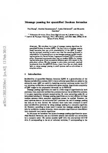
Domain size d=2 d=3 d≥4
δ value .7729 .6091 .5 + ²
Time bound 1.709m 1.953m dm/2+²m
when n > δm > 12 . The space complexity of the¡ second ¢ m stage is upper bounded by |F |·(n−δm)(m−δm) m−δm , since at any given time we only save the subformulas Table 1: Worst case upper bounds for quantified CSPs (C, i) for the current i. in terms of number of constraints. A well known result from ¡coding ¢theory says that m when δ > 12 , 2h(1−δ)m ≥ p(n) · (1−δ)m , where p(n) is a For Stage 2, we store subproblems here exactly how polynomial. From this and the fact that h(1−δ) = h(δ), we stored subformulas in the original algorithm. It the result follows. ¤ is not hard to see that for the subproblem (C, j), if some constraint c ∈ C contains the pair (vi , dk ), and The time is minimized when δ = h(δ), or δ ≈ .7729. i < j, then it must be that a(vi ) = dk in the (partial) Then, the time is O(1.709m ) and it is an improvement assignment a that led to C. This is an analogue of the subformula rule, and it means that by specifying (C, j), when m/n < 1.294. we may quickly determine the values of any variables vi Since h(δ) > δ for δ ≤ .7729, the above bound is (with i < j) that appear in C. optimal (for both time and space) when δ ≥ .7729. Notice that the previous running time bound of In this case, a tradeoff between time and space usage occurs. For example, when δ = .85, the algorithm runs Stage 2 works here. When δm variables have been set in O(1.906m ) time (the time for stage 1) and O(1.289m ) to values, it is still true that at least δm constraints have been already been satisfied, so we still only need space. to choose subsets of size at most m − δm. While we are achieving a better runtime, the exThus the running time is O(dδm + 2h(δ)m ), within ponential space bound can be somewhat costly. Later, we will discuss polynomial space algorithms for 3-CNF a polynomial factor. The following table gives times for several values of d, in comparison to brute-force search. quantified Boolean formulas. For d ≥ 4, our algorithm does not work optimally; this is because the optimal value for δ in this case is less than or equal to 1/2, and our results only hold for The dynamic programming technique does not rely δ < 1/2. Thus, for d ≥ 4, the bound is O(d(.5+²)m ), for heavily on specific properties of CNF Boolean formulas. ² > 0. It not surprising, then, that it can be used with quantified constraint satisfaction problems (QCSPs) in which the variables are quantified over a domain D of size d. 5 Algorithm for 3-CNF QBF 4.3
Generalization
Our constraint notation follows that of [7, 19]. A constraint is a set of pairs of the form (variable, value), and a CSP is a collection of constraints. A constraint c = {(vi1 , d1 ), . . . , (vik , dk )} is satisfied by an assignment a (a function from variables to domain D) if there is a pair (vij , dj ) ∈ c such that a(vij ) 6= dj . A QCSP of domain d and constraint size k is defined as a first-order sentence in prefix normal form, where the predicate of the sentence is a CSP of domain d with k variables per constraint. QCSPs may be thought of as two-player versions of the usual CSPs, where one player tries to satisfy the constraints, and an adversary tries to foil his attempt by setting “bad” values to variables.
By restricting ourselves to 3-CNF formulas, we find an improved time bound for QBF that requires only polynomial space. It is well known that 2-CNF QBF is polynomial time solvable [1]. Our idea is to branch in a such way that either two 3-CNF clauses are “reduced” to 2-CNF (or removed entirely), or more than just one variable is removed in one of the branches. A crucial observation we use has its origins with Monien and Speckenmeyer [12], and is essentially a reformulation of unit clause elimination. That is, given the QBF F ∧{li , lj }, with vi as the outermost quantified variable, if vi is existential/universal then F ∧ {li , lj } is true if and only if F [li := >] is true, or/and F [li := ⊥, lj := >] is true.
Stage 1 of our revised algorithm consists of dδm steps of trying possible solutions for the first δm variAdditionally, we use another rule in this algorithm: ables that are not trivially set by the rules, and removing constraints that are satisfied by these variable setRule 5.1. (Unit clause rule) tings.
5 For {lj } ∈ F , if li is universal, then F := ⊥. If li is existential, then set F := F − {c ∈ C : la ∈ c}. Like the monotone literal rule, unit clause was introduced with Davis-Putnam [6]. If a literal is universal and is the only literal of a clause, then any F containing this clause is false. If the literal is existential, it must be that li is true, if F is to be a true formula. 5.1
(3.2) If clauses of form {li , lj }, {li , lk }, {lj , lk , la } (or lj ,lk appear in separate 3-CNF clauses), then call the algorithm on: F with li := ⊥, lj := >, and F with li := >, lk := >. For each of these cases, if vi is universal (resp. existential), then return > iff both (resp. one of the) calls return >.
Algorithm
Given a QBF F ,
5.2
Apply monotone literal rule (4.3) and unit clause (5.1). If some clause is false, return ⊥. If all clauses are true, return >.
The proof of correctness is straightforward; cases 3.1 and 3.2 are sufficient since (C) takes care of the case where {lj , lk } is in F . Note that in cases 2.1 and 3.1, it is true that three distinct variables are set: if i = a or i = b, then these cases would already been eliminated by either rules (A), (B), or (C), a contradiction. It is obvious that the above algorithm requires only polynomial space.
Base cases: If there are no 3-CNF clauses in F , then solve the 2-CNF QBF and return its value. If n = 1, then try both values for the variable and return the value of F . (A) If there are clauses of the form {li , lj }, {li , lj }, and i < j, then replace vj (and vj ) with vi (vi ) in F . (B) If there are clauses of the form {li , lj }, {li , lj }, and i < j, then if vj is universal, return ⊥. Otherwise, set lj := >. (C) If clauses of form {li , lj }, {li , lk }, {lj , lk }, then replace vj (vj ) and vk (vk ) with vi (vi ). Let vi be the variable with the smallest index in F . There are five cases: (1) If there are clauses of the form {li , lj1 , lk1 } and {li , lj2 , lk2 }, then recursively call the algorithm on both: F with li := ⊥, and F with li := >. (2.1) If clauses of the form {li , lj1 , lk }, {li , lj2 }, and {lj2 , la }, call the algorithm on: F with li := ⊥, and F with li := lj2 := la := >. (2.2) If clauses of the form {li , lj1 , lk }, {li , lj2 }, and {lj2 , la , lb }, call the algorithm on: F with li := ⊥, and F with li := lj2 := >. (3.1) If clauses of form {li , lj }, {li , lk }, {lj , la }, {lk , lb }, then call the algorithm on: F with li := ⊥, lj := la := > and F with li := >, lk := lb := >.
Analysis
Let T (n, t) be the worst case running time of the algorithm for F when the number of 3-CNF clauses is t, and the number of variables is n. When case (1) is taken, the recurrence is bounded by 2T (n − 1, t − 2); one 3-CNF clause is reduced to 2-CNF, the other is removed entirely. For case (2.1), the time is less than T (n − 1, t − 1) + T (n − 3, t − 1). In case (2.2), it is T (n − 1, t − 1) + T (n − 2, t − 2), and for cases (3.1) and (3.2), it is 2T (n − 3, t) and 2T (n − 2, t − 1), respectively. Then we have the following double recurrence representing an upper bound on T : T (n, 0) = O(n2 ). T (1, t) = O(1). T (n, t) = max
2T (n − 1, t − 2), T (n − 1, t − 1)+ T (n − 3, t − 1), T (n − 1, t − 1)+ T (n − 2, t − 2), 2T (n − 3, t), 2T (n − 2, t − 1)
+ p(n),
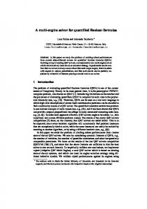
where p(n) is a polynomial representing the runtime of rule applications, (A)-(C), and case identification. We solved for values of the recurrence assuming t = cn, for some interesting values of c; the results are shown in Table 2. Notice that as the ratio of 3-CNF clauses to variables approaches 2, the running time approaches 2n . Due to space considerations, we only prove the t = n case. To disregard distracting polynomial factors in the analysis, we work with a simplified recurrence T 0 . Note that here we set T 0 (n, 1) as running in polynomial time,
6 t/n ratio c=1 c = 1.294 c = 1.4 c = 1.8 c=2
which is true in the algorithm (if a formula has one 3CNF clause, cases (1)-(3.2) are only considered once in the execution). This observation simplifies the proof. T 0 (n, i) = 1 for i ≤ 1, T 0 (j, t) = 1 for j ≤ 1. 2T 0 (n − 1, t − 2), T 0 (n − 1, t − 1) + T 0 (n − 3, t − 1), 0 T 0 (n − 1, t − 1) + T 0 (n − 2, t − 2), T (n, t) = max 2T 0 (n − 3, t), 2T 0 (n − 2, t − 1)
Theorem 5.1. T (n, n) = O(1.619n ). Proof. It will help us to prove the facts (1) If n < t, T 0 (n − 1, t) ≤ T 0 (n, t − 1), and (2) For n ≥ 5, T 0 (n, n − 1) = T 0 (n − 1, n − 2) + T 0 (n − 2, n − 3), simultaneously with (3) For n ≥ 3, T 0 (n, n) = T 0 (n − 1, n − 1) + T 0 (n − 2, n − 2), the Fibonacci reccurrence; this will imply the theorem since T 0 (n, n) = p(n) · T (n, n) for some sufficiently large polynomial p(n). First, fact (1) follows by induction on n + t. For the first four values of n + t, we observe that T (1, 2) = 1 ≤ 1 = T (2, 1), T (1, 3) = 1 ≤ 2 = T (2, 2), T (1, 4) = 1 ≤ 2 = T (2, 3). T (1, 5) = 1 ≤ 2 = T (2, 4) ≤ 3 = T (3, 3). Assume that (1) holds for n0 , t0 with 6 ≤ n0 + t0 < n + t. Then by induction: • 2T 0 (n − 2, t − 2) ≤ 2T 0 (n − 1, t − 3), • T 0 (n − 2, t − 1) + T 0 (n − 4, t − 1) ≤ T 0 (n − 1, t − 2) + T 0 (n − 3, t − 2), • T 0 (n − 2, t − 1) + T 0 (n − 3, t − 2) ≤ T 0 (n − 1, t − 2) + T 0 (n − 2, t − 3), • 2T 0 (n − 4, t) ≤ 2T 0 (n − 3, t − 1), and • 2T 0 (n − 3, t − 1) ≤ 2T 0 (n − 2, t − 2), which imply all together that T 0 (n − 1, t) ≤ T 0 (n, t − 1), by definition of T 0.
Time bound 3 · 1.619n = O(1.619n ) 2 · 1.524t = O(1.725n ) 2 · 1.4983t = O(1.762n ) 3 · 1.436t = O(1.919n ) 2 · 1.415t = O(2n )
. Table 2: Calculated bounds for the 3-CNF QBF algorithm. Now we simultaneously prove (2) and (3) by induction. For n = 5, T 0 (5, 4) = T 0 (4, 3) + T 0 (3, 2), and for n = 3, T 0 (2, 2) + T 0 (1, 1) = T (3, 3). For the inductive step, suppose facts (2) and (3) for any k < n. By induction, T 0 (n − 1, n − 2) = T 0 (n − 2, n − 3) + T 0 (n − 3, n − 4) by (2), so T 0 (n, n) = ½ max
2T 0 (n − 2, n − 3) + 2T 0 (n − 3, n − 4), T 0 (n − 1, n − 1) + T 0 (n − 2, n − 2)
¾ .
By definition of T 0 , 2T 0 (n−2, n−3) ≤ T 0 (n−1, n−1) and 2T 0 (n − 3, n − 4) ≤ T 0 (n − 2, n − 2), therefore T 0 (n, n) ≤ T 0 (n − 1, n − 1) + T 0 (n − 2, n − 2), and (3) holds. To (2), T (n − 1, n) = ¾ ½ prove 2T 0 (n − 2, n − 2), , max T 0 (n − 1, n − 2) + T 0 (n − 2, n − 3) and by induction on fact (3), 2T 0 (n − 2, n − 2) = 2T (n − 3, n − 3) + 2T 0 (n − 4, n − 4). 0
Again, by definition of T 0 , T 0 (n−1, n−2) ≥ 2T 0 (n− 3, n − 3) and T 0 (n − 2, n − 3) ≥ 2T 0 (n − 4, n − 4), so we conclude T (n − 1, n) ≤ T 0 (n − 1, n − 2) + T 0 (n − 2, n − 3). ¤
6
Solving 3-CNF Π2 -SAT
By considering more restrictive quantifications of variables, we obtain a better bound. The formulas in 3CNF Π2 -SAT consist of 3-CNF formulas F of the form: ∀u1 · · · ∀uj ∃xj+1 · · · ∃xn F . More formally, for some j, if i ≤ j then ui is a variable in F , and if i > j then xi is a variable.
We will say that a clause is i-universal if it contains exactly i universal literals. In solving 3-CNF Π2 -SAT, we may choose the order of what kind of clauses we Applying fact (1) to the terms in T 0 (n, n), T 0 (n − remove: 0, 1, or 2-universal. Since the quantification 3, n − 1) ≤ T 0 (n − 2, n − 2) and T 0 (n − 3, n) ≤ T 0 (n − consists of one set of universal variables followed by 2, n − 1) ≤ T 0 (n − 1, n − 2), so we find that existential variables, the strategy is clear: we efficiently ½ ¾ 0 eliminate the clauses containing universal variables, 2T (n − 1, n − 2), T 0 (n, n) = max . then solve the remaining 3-SAT instance. T 0 (n − 1, n − 1) + T 0 (n − 2, n − 2)
7 This algorithm uses another new rule: Rule 6.1. (Trivial falsity rule) If there is a clause c ∈ F containing only universal variables, then set F := ⊥. I.e. if a clause has no existential literals, this clause cannot possibly be satisfied in every case, so the subformula is false. This rule appears in Cadoli, et. al. [3] and in B¨ uning, et. al. [2]. 6.1
Algorithm
Given a 3-CNF Π2 -SAT instance F ,
We use the concept of branching tuples [11] (also called work factor) [7] to aid analysis. Let (t1 , . . . , tk ) be a tuple of integers, and define λ(t1 , . . . , tk ) as the Pk smallest positive root to the equation 1 − i=1 x1ti = 0. Suppose an algorithm has k separate recursive calls or “branches” within it (a la our algorithm above), and for the ith recursive call (i = 1, . . . , k), a measure µ of the input (e.g. µ = m or µ = n) is reduced to µ − ti . Assume these reductions take polynomial time each. From the work of Kullmann and Lockhardt [11], we find that the running time of this algorithm is at most T (µ) ≤
k X
[T (µ − ti ) + p(n)] ≤ q(n)λ(t1 , . . . , tk )µ ,
i=1
(0) If some clause is false, return ⊥. If all clauses are true, return >. Aply trivial falsity (rule 6.1), unit clause elimination (rule 5.1), and monotone literal (rule 4.3).
where p(n), q(n) are polynomials. This bound is O((λ(t1 , . . . , tk ) + ²)µ ), for any ² > 0. For example, an algorithm consisting of only case (1) above reduces n to (1) For each 2-universal 3-CNF clause {li , lj , lk } n − 1 for its first recursive call, n − 2 for its second, and with li and lj as universal, recursively call the algo- n − 3 for its third. Thus, this algorithm runs in time n rithm three separate times, with the following values bounded by (λ(1, 2, 3) + ²) . substituted in F for each call: Using branching tuples, we obtain the following li := >, and li := ⊥, lj := >, and li := lj := ⊥, lk := >. Return true iff all three calls return true.
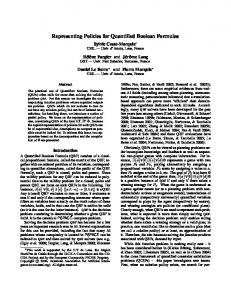
result: Theorem 6.1. Suppose m2 /n2 ≈ r, where m2 is the number of 2-universal 3-CNF clauses and n2 is the number of variables in these clauses. Then the above algorithm runs in time O(1.415m+(1.757/r−1)m2 ).
(2) [No 2-universal 3-CNF clauses for the rest of the computation.] For each 1-universal 2-CNF clause {li , lj } Proof. First, we remark that the cases of the algorithm with li as universal, call the algorithm twice separately, can be considered independently, in a sense. Once all with the following values substituted in F : 2-universal 3-CNF clauses have been considered and eliminated, case (1) no longer holds for the remainder of li := >, and the algorithm’s execution. The same holds for case (2) li := ⊥, lj := >. with respect to (3) and (4), and case (3) with respect to (4). Based on these observations, let ni represent Return true iff both calls return true. the number of variables of F considered during case (3) [No 2-universal clauses, and all 1-universal i of the algorithm, and mi be the number of 3-CNF clauses are 3-CNF.] For each 1-universal clause clauses eliminated (by being satisfied, or by becoming {li , lj , lk } with li as universal, try both possible values 2-CNF) in case i (so for example, m1 = m2 , m2 = 0). for li in the algorithm, and return true iff both values By considered, we mean that the variable appears in a lead to true. clause where the algorithm sets values to some or all of (4) Using Eppstein’s O(1.365t ) 3-SAT algorithm [7] the variables, depending on the branch. and return true iff the remaining 3-SAT instance is Due to this case independence, multiplying the time satisfiable. for (1) given above (in terms of n1 instead of n) with the time for (2), (3) and (4) gives a bound on the total 6.2 Analysis time. Independently of the others, case (2) requires time (λ(1, 2) + ²)n2 = O(1.619n2 ). The correctness of the above algorithm is easy to Let m0 be the number of 3-CNF clauses that have see, and so is the proof that it only uses polynomial been satisfied in a branch after cases (1) and (2) are space.
8 m2 /n2 r ≥ 1.757 r ≥ 1.4 r ≥ 1.294 r≥1
Time bound 1.415m 1.546m 1.603m 1.840m
Table 3: Bounds for 3-CNF Π2 -SAT algorithm. done, and n0 be the number of variables considered in these clauses. Clearly n0 = n1 + n2 , but also we claim that m0 ≥ m1 = m2 : if some 2-universal 3-CNF clause c is not satisfied after the execution of case (1), then a literal in c was falsified before our algorithm considered c. Either its existential literal was falsified (and trivial falsity would imply that F is false), or two universal literals were falsified (and unit clause elimination would satisfy the clause), or one universal literal was falsified. In that case, c becomes 1-universal 2-CNF, so it is then satisfied by case (2).
We now consider our results in relation to the fraction of QBFs that are conjectured to be the hardest, as claimed by Gent and Walsh [8]. They give two models for choosing random QBFs. Model A consists of choosing a 3-CNF Π2 -SAT instance at random, then discarding all 3-universal and 2-universal clauses. With this model, Gent and Walsh observe a phase transition of the “easy-hard-easy” type at m/n ≈ 2. That is, random instances generated by this model are true with high probability when either m/n < 2 and false with high probability when m/n > 2. The second model, Model B, constructs random 3CNF Π2 -SAT instances with m clauses and n variables by choosing two existential literals at random, then a universal variable, for each clause. The resulting formulas are of the same type as Model A, but the random choice produces an easy-hard-easy phase transition at a different point, m/n ≈ 1.4.
Our algorithm for 3-CNF Π2 -SAT works well in the absence of 2-universal clauses: if the only 3-CNF clauses Therefore, when considered independently of case m−m0 are 0 and 1-universal (so only cases (3) and (4) are (1) and (2), case (3) takes at most (λ(2, 2) + ²) ≤ m−m2 considered), the running time is O(2m1 /2 ·1.365m−m1 /2 ), (λ(2, 2)+²) time; with either recursive step of case (3), two 3-CNF clauses are eliminated. Consequently, where m1 is the number of 1-universal clauses. In the case (4) requires O(1.365m−m2 −m3 ) time, due to Epp- worst case, m = m1 and the bound is 1.415m . This stein’s 3-SAT algorithm based on the number of 3-CNF implies that the algorithm runs in time better than 2n when m/n < 2, for all formulas that may be chosen out clauses [7]. of Model A or Model B. Hence the “easily true” instances In the worst situation, case (4) is never considered, from both models can be solved in time less than 2n , and all of the clauses are removed by cases (1), (2), and using our Π -SAT algorithm. Notably, for m/n ≈ 1.4 2 (3), because 1.365 < 1.415 ≈ λ(2, 2) + ², for sufficiently (the phase transition point for Model A), the algorithm small ² > 0. Initially, every clause of F is 3-CNF, runs in time O(1.625n ). so each 1-universal 2-CNF clause {lj , lk } considered by case (2) was originally some 2-universal 3-CNF clause {li , lj , lk } reduced by case (1). This implies that the 7 Conclusions number of variables in 2-universal 3-CNF clauses is at least the number considered in case (1) and (2), i.e. We have seen various ways in which QBF algorithms can be devised: using dynamic programming, transforn2 ≥ n1 + n2 , for all branches of the algorithm. mation rules, and pieces of existing SAT algorithms. Then, the running time is bounded by 1.840n2 · The algorithms presented are simple yet effective, as to 1.619n1 · 1.415m−m2 = O(1.840n2 · 1.415m−m2 ). provide a solid starting point in research towards imWhen m2 /n2 ≈ r, then the time is at most proved algorithms for QBF. Here are a few suggestions 1.415log(1.840)/ log(1.415)m2 /r+m−m2 , or more compactly, for further study. O(1.415(1.757/r−1)m2 +m ). ¤ • Recall that the proof for the time bound on the arbitrary CNF QBF algorithm only uses the first As the clause-to-variable ratio for the 2-universal three transformation rules given (subformula, contraclauses increases, the running time decreases. Note diction/truth, and monotone literal). This bound can that this is an opposite effect from the 3-CNF QBF probably be significantly improved by using more of algorithm. Table 3 quantitatively demonstrates the these rules in our reasoning. tradeoff between clause-to-variable ratio and running • It is interesting that in practice, 2-universal time. clauses in 3-CNF Π2 -SAT were not considered in evaluating “hard” formulas [8], yet the time bound for our algorithm is hampered by their presence. Perhaps an 6.3 Relation with the QBF phase transition
9 interleaving of this algorithm with one closer to the experimental algorithms (which do well with 2-universal clauses) would give a solid O(1.414m ) bound, or better. • Our algorithms set the values for variables according to their order, except when a variable is forced to be a value (due to the rules). However, it is possible that some QBF solvers need not preserve the order of quantification when they set variables. For example, consider ∀y1 · · · yk ∃z F . We could set z := >, keeping a record of those yi -values with which z := > works. Then when z := ⊥ is considered, we ensure that if some value of y does not work in this case, then it worked when z := >. Rintanen [16] describes a similar procedure he calls quantifier inversion. However, his randomized strategy for changing the order of the variables appears difficult to analyze rigorously. • It seems plausible that a variation on local search could be implemented for Π2 -SAT. The search could have two phases: one in which a search for a “bad” assignment of universal variables ensues, and one in which a satisfying assignment of the existential variables is found, given the candidate universal assignment. One heuristic for local change towards a “bad” assignment is: if there exists a clause c such that exactly one of its literals li is true and li is universal, flip the variable value of ui . (Such a clause and literal exist, otherwise the formula is true if it is satisfied by the current existential assignment.) 8
[6]
[7]
[8] [9]
[10]
[11]
[12]
[13]
[14]
[15]
Acknowledgements
I am indebted to Dieter van Melkebeek and Eva Tardos for their generous comments and suggestions on drafts of this paper. References [1] B. Apswall, M. F. Plass and R. E. Tarjan, A lineartime algorithm for testing the truth of certain quantified Boolean formulas, Information Processing Letters, 8:121-123, 1979. [2] H. K. Buning, M. Karpinski, and A. Flogel, Resolution for quantified Boolean formulas, Information and Computation, 117(1):12-18, 1995. [3] M. Cadoli, A. Giovanardi, and M. Schaerf, An algorithm to evaluate quantified Boolean formulae, Proceedings of AAAI-98, pp. 262-267, 1998. [4] J. Chen, I. A. Kanj, and W. Jia, Vertex cover: Further observation and further improvements, Lecture Notes in Computer Science 1665 (WG’99), Springer-Verlag, Berlin, pp. 313-324, 1999. [5] E. Dantsin, A. Goerdt, E. A. Hirsch, R. Kannan, J. Kleinberg, C. Papadimitriou, P. Raghavan, U. 2 )n algorithm for Sch¨ oning, A deterministic (2 − k+1
[16]
[17]
[18]
[19]
k-SAT based on local search, Accepted in Theoretical Computer Science, 2001. M. Davis and H. Putnam, A computing procedure for quantification theory, Journal of the ACM, 7(1):201215, 1960. D. Eppstein, Improved Algorithms for 3-Coloring, 3Edge-Coloring, and Constraint Satisfaction, Proceedings of 12th ACM-SIAM Symposium on Discrete Algorithms, pp. 329-337, 2001. I. Gent and T. Walsh, Beyond NP: the QSAT phase transition, Proceedings of AAAI-99, 1999. E. Giunchiglia, M. Narizzano, and A. Tacchella. QUBE: A system for deciding quantified Boolean formulas satisfiability, Proceedings of the Int. Joint Conference on Automated Reasoning, 2001. E. A. Hirsch. New worst-case upper bounds for SAT, Journal of Automated Reasoning, 24(4): 397-420, 2000. O. Kullmann and H. Luckhardt, Deciding propositional tautologies: algorithms and their complexity, http://www.cs.toronto.edu/~kullmann. B. Monien and E. Speckenmeyer, Solving satisfiability in less than 2n steps, Discrete Applied Mathematics, 10:287-295, 1985. R. Paturi, P. Pudlak, and F. Zane, Satisfiability coding lemma, Proceedings of 38th IEEE Symposium on Foundations of Comp. Sci., pp. 566-574, 1997. R. Paturi, P. Pudlak, M. E. Saks, and F. Zane. An improved exponential-time algorithm for k-SAT, Proceedings of 39th IEEE Symposium on Foundations of Comp. Sci., pp. 628-637, 1998. R. Rodosek, A new approach on solving 3-satisfiability, Proceedings of 3rd Int. Conference on AI and Symbolic Mathematical Computing, Springer-Verlag, LNCS 1138, pp. 197-212, 1996. J. Rintanen, Improvements to the evaluation of quantified Boolean formulae, 16th Int. Joint Conference on AI, pp. 1192-1197, 1999. J. Rintanen, Partial implicit unfolding in the DavisPutnam procedure for quantified Boolean formulas, Workshop on Theory and Applications of QBF, Int. Joint Conference on Automated Reasoning, 2001. R. Schuler, U. Sch¨ oning, and O. Watanabe, An improved randomized algorithm for 3-SAT, Technical Report TR-C146, Dept. of Mathematical and Computing Sci., Tokyo Inst. of Tech., 2001. U. Sch¨ oning, A probabilistic algorithm for k-SAT and constraint satisfaction problems, Proceedings of 40th IEEE Symposoum on Foundations of Comp. Sci., pp. 410-414, 1999.