berg, a generalisation of finite state automata suitable for general non- deterministic computation. Such machines complement an automaton, seen as its control ...
Computing with Relational Machines G´erard Huet and Benoˆıt Razet INRIA Paris-Rocquencourt ICON’2008 Tutorial, Pune, December 2008
Abstract. We give a quick presentation of the X-machines of Eilenberg, a generalisation of finite state automata suitable for general nondeterministic computation. Such machines complement an automaton, seen as its control component, with a computation component over a data domain specified as an action algebra. Actions are interpreted as binary relations over the data domain, structured by regular expression operations. We show various strategies for the sequential simulation of our relational machines, using variants of the reaction engine. In a particular case of finite machines, we show that bottom-up search yields an efficient complete simulator. Relational machines may be composed in a modular fashion, since atomic actions of one machine may be mapped to the characteristic relation of other relational machines acting as its parameters. The control components of machines is compiled from regular expressions. Several such translations have been proposed in the literature, that we briefly survey. Our view of machines is completely applicative. They may be defined constructively in type theory, where the correctness of their simulation may be formally checked. From formal proofs in the Coq proof assistant, efficient functional programs in the Objective Caml programming language may be mechanically extracted. Most of this material is extracted from the (forthcoming) Ph.D. thesis of Benoˆıt Razet.
1 1.1
Machines Relational machines
We shall define a notion of abstract machine inspired from the work of Eilenberg (X-machines, presented in [8]). Our machines are non-deterministic in nature. They comprise a control component, similar to the transitions state diagram of a (non-deterministic) automaton. These transitions are labeled by action generators. Action expressions over free generators, generalizing regular expressions from the theory of languages, provide a specification language for the control component of machines. A program, or action expression, compiles into control components according to various translations. Control components in their turn may compile further into transition matrices or other representations.
2
Our machines also comprise a data component, endowed with a relational semantics. That is, we interpret action generators by semantic attachments to binary relations over the data domain. These relations are themselves represented as functions from data elements to streams of data elements. This applicative apparatus replaces by clear mathematical notions the imperative components of traditional automata (tapes, reading head, counters, stacks, etc). We shall now formalise these notions in a way which will exhibit the symmetry between control and data. First of all, we postulate a finite set Σ of parameters standing for the names of the primitive operations of the machine, called generators. For the control component, we postulate a finite set S of states and a transition relation map interpreting each generator as a (binary) relation over S. This transition relation interpretation is usually presented currified as a transition function δ mapping each state in S to a finite set of pairs (a, q) with a a generator and q a state. This set is implemented as a finite list of such pairs. Finally, we select in S a set of initial states and a set of accepting states. For the data component, we postulate a set D of data values and a computation relation map interpreting each generator as a (binary) relation over D. Similarly as for the control component, we shall currify this relation map as a computation function mapping each generator a in Σ to a function ρ(a) in D → ℘(D). Now the situation is not like for control, since D and thus ℘(D) may be infinite. In order to have a constructive characterization, we shall assume that D is recursively enumerable, and that each ρ(a) maps d ∈ D to a recursively enumerable subset of ℘(D). We shall represent such subsets as progressively computed streams of values, as we shall explain in due time. 1.2
Progressive relations as streams
We recall that a recursively enumerable subset of ω is the range of a partial recursive function in ω ⇀ ω, or equivalently it is either empty or the range of a (total) recursive function in ω → ω. None of these two definitions is totally satisfying, since in the first definition we may loop on some values of the parameter, obliging us to dovetail the computations in order to obtain a sequence of elements which enumerates completely the set, and in the second we may stutter enumerating the same element in multiple ways. This stuttering cannot be totally eliminated without looping, for instance for finite sets. Furthermore, demanding total functions is a bit illusory. It means either we restrict ourserves to a non Turing-complete algorithmic description language (such as primitive recursive programs), or else we cannot decide the totality of algorithms demanded by the definition. We shall here assume that our algorithmic description language is ML, i.e. typed lambda-calculus evaluated in call by value with a recursion operator, inductive types and parametric modules. More precisely, we shall present all our algorithms in the Objective Caml implementation. In this framework we may define computable streams over a parametric datatype data as follows:
3
type stream ’data = [ Void | Stream of ’data and delay ’data ] and delay ’data = unit → stream ’data; This expresses that a stream of data values is either Void, representing the empty set, or else a pair Stream(d,f) with d of type data, and f a frozen stream value, representing the set {d}∪F , where F may be computed as the stream f (), where () is syntax for the canonical element in type unit. Using this inductive parametric datatype, we may now define progressive relations by the following type: type relation ’data = ’data → stream ’data;
1.3
Kernel machines
We now have all the ingredients to define the module signature of kernel machines: module type EMK = sig type generator; type data; type state; value transition: state → list (generator × state); value initial: list state; value accept: state → bool; value semantics : generator → relation data; end; In the following, we shall continue to use Σ (resp. D, S, δ, ρ) as shorthand for generator (resp. date, state, transition, semantics). We also write I for initial and T for the set of accepting states (for which the predicate accept is true). A machine is like a blackbox, which evolves through series of non-deterministic computation steps. At any point of the computation, its status is characterized by the pair (s, d) of its current state s ∈ S and its current data value d ∈ D. Such a pair is called a cell. A computation step issued from cell (s, d) consists in choosing a transition (a, s′ ) ∈ δ(s) and a value d′ ∈ ρ(a)(d). If any of these choices fails, because the corresponding set is empty, the machine is said to be blocked; otherwise, the computation step succeeds, and the machine has as status the new cell (s′ , d′ ). a We write (s, d) → (s′ , d′ ). A computation path consists of such computations steps: a
a
a
n (sn , dn ) (s0 , d0 ) →1 (s1 , d1 ) →2 (s2 , d2 )... →
4
The computation is said to be accepting whenever s0 ∈ I and sn ∈ T , in which case we say that the machine accepts input d0 and computes output dn . Remark that (d0 , dn ) belongs to the graph of the composition of relations labeling the path: ρ(a1 ) ◦ ρ(a2 ) ◦ ...ρ(an ). We have thus a very general model of relational calculus. Our machines compute relations over the data domain D, and we shall thus speak of D-machines. The “machine language” has for instructions the action generators. Actions compose by computation. Furthermore, a high level programming language for relational calculus may be designed as an action calculus. The obvious point of departure for this calculus is to consider regular expressions, in other words the free Kleene algebra generated by the set of generators. We know from automata theory various translations from regular expressions to finite-state automata. Every such translation gives us a compiler of our action algebra into the control components of our machines: S, δ, I and T . The data components, D and ρ, offer a clean mathematical abstraction over the imperative paraphernalia of classical automata: reading heads, tapes, etc. And we get immediately a programming language enriching the machine language of primitive actions by composition, iteration, and choice. Indeed, a finite automaton over alphabet Σ is readily emulated by the machine with generator set Σ having its state transition graph as its control component, and having for data domain the free monoid of actions Σ ∗ . Each generator a is interpreted in the semantics as the (functional) relation ρ(a) = L−1 a =def {(a · w, w) | w ∈ Σ ∗ } which “reads the input tape”. And indeed the language recognized by the automaton is retrieved as the composition of actions along all accepting computations. Here the data computation is merely a trace of the different states of the “input tape”. This example is a simple one, and data computation is deterministic, since ρ(a) is a partial function. We may say that such a machine is “data driven”. Control will be deterministic too, provided the underlying automaton is deterministic, since every δ(s) will then have a unique non-blocking transition. But remark that the same control component may be associated with different semantics. For instance, with ρ(a) = Ra =def {(w, w · a) | w ∈ Γ ∗ }, the machine will enumerate with its accepting computations the regular language recognized by the automaton. Let us now turn towards the action calculus.
2
Actions
Actions may be composed. We write A · B for the composition of actions A and B. This corresponds to the composition of the underlying relations. Actions may be iterated. We write A+ for the iteration of action A. This corresponds to the transitive closure of the underlying relation. We postulate an identity action 1 corresponding to the underlying identity relation.
5
Actions may be summed. We write A + B for the sum of actions A and B. This corresponds to the union of the underlying relations. We note A∗ for 1+A+ . We also postulate an empty action 0. The algebraic structure of actions is that of a composition monoid: (A · B) · C = A · (B · C) A·1= 1·A =A and for union, an idempotent abelian monoid: (A + B) + C = A + (B + C) A+B =B+A A+0=0+A=A A+A =A verifying distributivity: A · (B + C) = A · B + A · C (A + B) · C = A · C + B · C A·0 =0·A= 0 and thus, so far actions form an idempotent semiring. Defining A ≤ B =def A + B = B, the partial ordering ≤ makes the algebra of actions an upper semilattice. As for iteration (which will be interpreted over relations by transitive-reflexive closure), we follow Pratt [15] in adding implications between actions, in order to get an algebraic variety (as opposed to Kleene algebras, which only form a quasi variety, i.e. need conditional identities for their complete axiomatisation). Thus we postulate ← and →, corresponding to relational semi-complements: ρ → σ = {(v, w) | ∀u uρv ⇒ uσw} σ ← ρ = {(u, w) | ∀v wρv ⇒ uσv} and we axiomatise actions as residuation algebras, following Kozen [14]: A·C ≤B ⇔C ≤A→B C ·A≤B ⇔C ≤B ←A or alternatively we may replace these two equivalences by the following equational axioms: A · (A → B) ≤ B (B ← A) · A ≤ B A → B ≤ A → (B + C)
6
B ← A ≤ (B + C) ← A A ≤ B → (B · A) A ≤ (A · B) ← B We may now get Pratt’s action algebras by axiomatizing iteration as pure induction: 1 + A + A∗ · A∗ ≤ A∗ (A → A)∗ = A → A (A ← A)∗ = A ← A The residuation/implication operations may be seen as the right interpolants to extend conservatively Kleene algebras to the variety of action algebras. Regular expressions and their compilation extend gracefully to action expressions, and the residuation operations correspond to Brzozowki’s derivatives. Furthermore, following Kozen [14], we may wish to enrich our actions with a multiplicative operation ∩, corresponding to relation intersection, verifying lower semilattice axioms: (A ∩ B) ∩ C = A ∩ (B ∩ C) A∩B =B ∩A A∩A=A and completing to a lattice structure with: A + (A ∩ B) = A A ∩ (A + B) = A obtaining thus Kozen’s action lattices, the right structure for matrix computation. We remark that such structures go in the direction of logical languages, since union, intersection and residuation laws are valid Heyting algebras axioms. We are still far from the complete Boolean algebra structure of relations, though.
3
Behaviour and interfaces
We recall that we defined above the accepting computations of a machine, and for each such computation its compound action, obtained by composing the generating relations of each computation step. Let us call behaviour of a machine M the set of all such compound actions, noted |M|. Now we define the characteristic relation of a machine M as the union of the semantics of its behaviour: [ ρ(a) ||M|| = a∈|M|
Characteristic relations are the relational interpretation over the data domain D of the action langage recognized by the underlying automaton. They allow us to compose our machines in modular fashion.
7
3.1
Modular construction of machines
Now that we understand that a D-machine implements a relation over D, we may compose machines vertically, as follows. Let A be a (non-deterministic) automaton over alphabet Σ, and for every a ∈ Σ let Na be a D-machine over some generator set Σa . We may now turn A into a D-machine over generator set Σ by taking A as its control component, and extending it by a data component having as semantics the function mapping a ∈ Σ to ||Na ||. We may thus construct large machines from smaller ones computing on the same data domain. A typical example of application for computational linguistics is to do morphological treatment (such as segmentation and tagging of some corpus) in a lexicon-directed way. The alphabet Σ defines the lexical categories or parts of speech, each machine Na implements access to the lexicon of category a, the automaton A defines the morphological geometry, and the composite machine M implements a lexicon-directed parts-of-speech tagger. By appropriate extension of the lexicon machines Na , morpho-phonemic treatment at the junction of the words may be effected, such as complete sandhi analysis for Sanskrit [11, 12]. 3.2
Interfaces
What we described so far is the Eilenberg machine kernel, consisting of its control and data elements. We may complete this description by an interface, composed of an input domain D− , an output domain D+ , an input relation φ− and an output relation φ+ . A machine M completed by this interface I defines a relation φ(M, I) : D− → D+ by composition: φ(M, I) = φ− ◦ ||M|| ◦ φ+
4
Finite machines
We shall now present an important special case of machines which exhibit a finite behaviour. The relation ρ : D → D′ is said to be locally finite if for every d ∈ D the set ρ(d) is finite. The machine M is said locally finite if every relation ρ(a) is locally finite [9]. The machine M is said nœtherian if all its computations are finite in length. We remark that a machine is nœtherian when its data domain D is a wellfounded ordering for the order relation > generated by: d > d′ ⇐ ∃a ∈ Σ d′ ∈ ρ(a)(d) Indeed, if there existed an infinite computation, there would exist an infinite sub-sequence going through the same state. But the converse is not true, since a machine may terminate for a reason depending of its control. Finally, we say that a machine is finite if it is locally finite and nœtherian.
8
We say that a machine is sequential [8] iff for each cell value (s, d) occurring in a computation there exists at most one computation transition issued from it, i.e. if δ(s) is a set of pairs {(ρ1 , s1 ), (ρ2 , s2 ), ...(ρn , sn )} such that for at most one 1 ≤ k ≤ n the set ρk (d) is non empty, and if such k exists then ρk (d) is a singleton. This condition demands that on one hand the transition relation of the underlying automaton is a partial function, that is the automaton must be deterministic, and on the other hand that the relations leading out of a state s be partial functions over the subset of D which is reachable by computation leading to s. We remark that a sequential machine may nevertheless generate several solutions, since a terminal cell is not necessarily blocking further computation. 4.1
Examples
Non deterministic finite automata Let us consider a non-deterministic automaton A with parameters (S, I, T, δ). We construct an Eilenberg machine M solving the word problem for the rational language |A| recognized by the automaton. M has Σ for generating set, and it takes A for its control component. For the data component, we take D = Σ ∗ , and the semantics is ρ(a) = L−1 a =def {(a · w, w) | w ∈ Σ ∗ }, as explained above. We may check that ρ(w) = 1 iff w ∈ |A|. It is easy to check that M is finite, since data decreases in length, and semantics is a partial function. When A is a deterministic automaton, M is a sequential machine. Another machine with the same control component may be defined to enumerate all the words in set |A|. In general it will neither be finite, nor sequential. Rational transducers Let Σ and Γ be two finite alphabets. A transducer A : Σ ⇒ Γ is similar to a (non-deterministic) automaton, whose transitions are labeled with pairs of words in D = Σ ∗ × Γ ∗ . Let Ω be the (finite) set of labels occurring as labels of the transitions of A. The transition graph of A may thus be considered as an ordinary non-deterministic automaton over generator alphabet Ω, and constitutes the control component of the machines we shall define to solve various transductions tasks. We recall that a transducer “reads its input” on an input tape representing a word in Σ ∗ and “prints its output” on an output tape representing a word in Γ ∗ . On transition (w, w′ ) it reads off w on the input tape, and if successful appends w′ to its output tape. If by a succession of transitions starting from an initial state with input i and empty output it reaches an accepting state with empty input and output o, we say that (i, o) belongs to the rational relation in Σ ⇒ Γ recognized by the transducer A, which we shall write |A|. We shall now solve various decision problems on |A| using machines which use A for control and D for data, but replace the tapes by various semantic functions: 1. Recognition. Given (w, w′ ) ∈ D, decide whether (w, w′ ) ∈ |A|. 2. Synthesis. Given w ∈ Σ ∗ , compute its image |A|(w) ⊂ Γ ∗ . 3. Analysis. Given w ∈ Γ ∗ , compute the inverse image |A−1 |(w) ⊂ Σ ∗ .
9 −1 Recognition. The semantics ρ is defined by ρ(σ, γ) = L−1 σ × Lγ . Like for ordinary automata we obtain a finite machine, provided the transducer has no transition labeled (ǫ, ǫ), since at least one of the two lengths decreases. We choose as interface D− = Σ ∗ × Γ ∗ , φ− = IdΣ ∗ ×Γ ∗ , D+ = 0, 1, φ+ (w, w′ ) = 1 iff w = w′ = ǫ. Synthesis. The semantics ρ is defined by ρ(σ, γ) = L−1 σ × Rγ , with Rγ =def {(w, w · γ) | w ∈ Γ ∗ }. We choose as interface D− = Σ ∗ , φ− = {(w, (w, ǫ)) | w ∈ Σ ∗ }, D+ = Γ ∗ , φ+ = {(ǫ, w′ ), w′ ) | w′ ∈ Γ ∗ }. We get |A| = φ− ◦ ||M|| ◦ φ+ . Such a machine is locally finite, since relations L−1 σ and Rγ are partial functions. However, it may not be nœtherian, since there may exist transitions labeled with actions (ǫ, w). Actually the machine is nœtherian iff cycles of such transitions do not occur, iff the set |A|(w) is finite for every w ∈ Σ ∗ [16]. −1 Analysis. Symmetric to synthesis, replacing L−1 σ by Rσ and Rγ by Lγ .
Oracle machines Let D be an arbitrary set, and P an arbitarry predicate over D. We consider the relation ρ over D defined as the restriction of identity to the data elements verifying P : ρ(d) = {d} if P (d), ρ(d) = ∅ otherwise. We define in a canonical way the machine whose control component is the automaton A with two states S = {0, 1}, I = {0} and T = {1}, and transition function δ defined by δ(0) = {(ρ, 1)} and δ(1) = ∅. This machine is a sequential finite machine, that decides in one computational step whether its input verifies P . Our restriction of Eilenberg machines to computable relations limits such oracles to recursive predicates, but of arbitrary complexity. More generally, our machines recursively enumerate arbitrary recursively enumerable sets, and are therefore Turing complete.
5
Reactive engine
We may simulate the computations of a finite Eilenberg machine by adapting the notion de reactive engine of the Zen library [10–12, 16]. 5.1
The depth-first search reactive engine
module Engine (Machine: EMK) = struct open Machine; type choice = list (generator × state); (* We stack backtrack choice points in a resumption *) type backtrack = [ React of data and state | Choose of data and choice and delay data and state ] and resumption = list backtrack;
10
(* The 3 internal loops of the reactive engine *) (* react: data → state → resumption → stream data *) value rec react d q res = let ch = transition q in (* we need to compute [choose d ch res] but first we deliver data [d] to the stream of solutions when [q] is accepting *) if accept q then Stream d (fun () → choose d ch res) (* Solution d found *) else choose d ch res (* choose: data → choice → resumption → stream data *) and choose d ch res = match ch with [ [] → resume res | [ (g, q’) :: rest ] → match semantics g d with [ Void → choose d rest res | Stream d’ del → react d’ q’ [ Choose d rest del q’ :: res ] ] ] (* The scheduler which backtracks in depth-first exploration *) (* resume: resumption → stream data *) and resume res = match res with [ [] → Void | [ React d q :: rest ] → react d q rest | [ Choose d ch del q’ :: rest ] → match del () with (* we unfreeze the delayed stream of solutions *) [ Void → choose d ch rest (* finally we look for next pending choice *) | Stream d’ del’ → react d’ q’ [ Choose d ch del’ q’ :: rest ] ] ] ; (* Note that these are just loops, since the recursive calls are terminal *) (* Simulating the characteristic relation: relation data *) value simulation d = let rec init_res l acc = match l with [ [] → acc | [ q :: rest ] → init_res rest [ React d q :: acc ] ] in
11
resume (init_res initial []) ; end; (* module Engine *) 5.2
Correctness, completeness, certification
Benoˆıt Razet showed in [17] a formal proof of correctness and completeness of the simulation of a finite machine by the above reactive engine. Furthermore, it is possible to extract mechanically from this proof ML algorithms identical to the ones we showed above. 5.3
A General reactive engine, driven by a strategy
When a machine is not finite, and in particular when there are infinite computation paths, the bottom-up engine above may loop, and the simulation is not complete. In order to remedy this, we shall change the fixed last-in first-out policy of resumption management, and replace it by a more general strategy given as a parameter of the machine. open Eilenberg; module Engine (Machine: EMK) = struct open Machine; type choice = list (generator × state); (* We separate the control choices and the data relation choices *) type backtrack = [ React of data and state | Choose of data and choice | Relate of stream data and state ] ; Now resumption is an abstract data type, given in a module Resumption, passed as argument to the Strategy functor, generalizing a backtrack stack. module Strategy (* resumption management *) (Resumption : sig type resumption; value empty: resumption; value pop: resumption → option (backtrack × resumption); value push: backtrack → resumption → resumption; end) = struct open Resumption;
12
Now we define a more parametric reactive engine, using an exploration strategy as parameter. (* react: data → state → resumption → stream data *) value rec react d q res = let ch = transition q in if accept q (* Solution d found? *) then Stream d (fun () → resume (push (Choose d ch) res)) else resume (push (Choose d ch) res) (* choose: data → choice → resumption → stream data *) and choose d ch res = match ch with [ [] → resume res | [ (g, q’) :: rest ] → let res’ = push (Choose d rest) res in relate (semantics g d) q’ res’ ] (* relate: stream data → state → resumption → stream data *) and relate str q res = match str with [ Void → resume res | Stream d del → let str = del () in resume (push (React d q) (push (Relate str q) res)) ] (* resume: resumption → stream data *) and resume res = match pop res with [ None → Void | Some (b, rest) → match b with [ React d q → react d q rest | Choose d ch → choose d ch rest | Relate str q → relate str q rest ] ] ; (* characteristic_relation: relation data *) value simulation d = let rec init_res l acc = match l with [ [] → acc | [ q :: rest ] → init_res rest (push (React d q) acc)
13
] in resume (init_res initial empty) ; end; (* module Strategy *)
5.4
A few typical strategies
We now give a few variations on search strategies. First of all, we show how the original depth-first reactive engine may be obtained by a DepthFirst strategy module, adequate for Finite Eilenberg Machines. module DepthFirst = struct type resumption = list backtrack; value empty = []; value push b res = [ b :: res ]; value pop res = match res with [ [] → None | [ b :: rest ] → Some (b,rest) ]; end; (* module DepthFirst *) Next we examine the special case of sequential machines, where computations are deterministic. The following simple Seq tactic is adapted to this case. module Seq = struct type resumption = list backtrack; value empty = []; value push b res = match b with [ React _ _ → [ b :: res ] | Choose _ _ → [ b ] (* cut : the list contains only one element *) | Relate _ _ → res (* no other delay *) ]; value pop res = match res with [ [] → None | [ b :: rest ] → Some (b,rest) ]; end; (* module Seq *) Finally, we show how to simulate in a fair way a general machine with a Complete tactic, which scans the state space in a top-down boustrophedon manner. module Complete = struct type resumption = (list backtrack × list backtrack);
14
value empty = ([],[]); value push b res = let (left,right) = res in (left, [ b :: right ]) ; value pop res = let (left,right) = res in match left with [ [] → match right with [ [] → None | [ r :: rrest ] → Some (r, (rrest,[])) ] | [ l :: lrest ] → Some (l, (lrest,right)) ] ; end; (* module Complete *) Now we may build the various modules encapsulating the various strategies. module FEM = Strategy DepthFirst; (* The bottom-up engine *) module Sequential_Engine = Strategy Seq; (* The sequential engine *) module Complete_Engine = Strategy Complete; (* The fair engine *) end; (* module Engine *)
6
From regular expressions to automata
Our motivation here is the design of a language for describing the control part of Eilenberg machines. The control part of Eilenberg machines is a finite automaton. It leads us naturally to regular expressions and their translations into finite automata. There have been more than 50 years of research on the problem of compilation (or translation) of regular expressions into automata. It started with Kleene who stated the equivalence between the class of languages recognized by finite automata and the class of languages defined by regular expressions. This topic is particularly fruitful because it has applications to string search algorithms, circuits, synchronous languages, computational linguistics, etc. This wide range of applications leads to several automata and regular expressions variants. Usually, an algorithm compiling regular expressions into automata is described in an imperative programming style for managing states and edges: states are allocated, merged or removed and so on concerning the edges. Surprisingly it seems that there is an applicative manner for describing each of the well-known algorithms. This methodology leads to a formal definition of the algorithm exhibiting important invariants. Of course we are careful to maintain the theoretical complexity of the algorithms.
15
We focus on fast translations, whose time complexity is linear or quadratic with respect to the size of the regular expression. First we present Thompson’s algorithm [18] and then we review other algorithms that are concerned by our methodology. Let us mention Brzozowski’s algorithm [5] which translates a regular expression (even with boolean operators) into a deterministic automaton. Unfortunately, the complexity is theoretically exponential. Nevertheless, it introduced the notion of regular expression derivative which is a fundamental idea pervading other algorithms. 6.1
Thompson’s algorithm
Thompson presented his algorithm in 1968 and it is one of the most famous translations. It computes a finite non-deterministic automaton with ǫ-moves in linear time. Let us first define regular expressions as the following datatype: type regexp ’a = [ One | Symb of ’a | Union of regexp ’a and regexp ’a | Conc of regexp ’a and regexp ’a | Star of regexp ’a ]; The constructor One of arity 0 is for the 1 element of the corresponding action algebra. The following constructor Symb of arity 1 is the node for a generator. The type for the generator is abstract as expressed by the type parameter ’a in the definition. The two following constructors are Union and Conc of arity 2 and describe union and concatenation operations. The last constructor Star is for the iteration or Kleene’s star operator. Now we have given the datatype for the input of our algorithm, let us present the datatype for the output (automata). We choose to implement states of the automaton with integers: type state = int; Automata obtained by Thompson’s algorithm are non-deterministic and furthermore with ǫ-moves. We shall implement the control graph of such nondeterministic automata as a list of fanout pairs associating a list of labeled a transitions to a state. This amounts to encoding a set of edges s → s′ or triples ′ (s, a, s ) as an association list. type fanout ’a = (state * list (label ’a * state)) and label ’a = option ’a and transitions ’a = list (fanout ’a) ; type automaton ’a = (state * transitions ’a * state);
16
A label is of type option ’a because it may be either an ǫ-move of value None or a generator a of value Some a. Note that even if they are non-deterministic, the automata we consider have only one initial and one accepting state. We shall instanciate the transition function of the control component of our machines by composing the transitions list component of the constructed automaton with the primitive List.assoc, as we shall show later in section 7. Thompson’s algorithm can be summarized very shortly in a graphical way:
The algorithm performs a recursive traversal of the expression and each case corresponds to a drawing. It is presented in the order of the datatype definition: 1, generator, union, concatenation and Kleene’s star. (* thompson: regexp ’a → automaton ’a *) value thompson e = let rec aux e t n = (* e is current regexp, t accumulates the state space, n is last created location *) match e with [ One → let n1=n+1 and n2=n+2 in (n1, [ (n1, [ (None, n2) ]) :: t ], n2) | Symb s → let n1=n+1 and n2=n+2 in (n1, [ (n1, [ (Some s, n2) ]) :: t ], n2) | Union e1 e2 → let (i1,t1,f1) = aux e1 t n in let (i2,t2,f2) = aux e2 t1 f1 in let n1=f2+1 and n2=f2+2 in (n1, [ (n1, [ (None, i1); (None, i2) ]) :: [ (f1, [ (None, n2) ]) :: [ (f2, [ (None, n2) ]) :: t2 ] ] ], n2) | Conc e1 e2 → let (i1,t1,f1) = aux e1 t n in let (i2,t2,f2) = aux e2 t1 f1 in
17
(i1, [ (f1, [ (None, i2) ]) :: t2 ], f2) | Star e1 → let (i1,t1,f1) = aux e1 t n in let n1=f1+1 and n2=f1+2 in let t1’ = [ (f1, [ (None, i1); (None, n2) ]) :: t1 ] in (n1, [ (n1, [ (None, i1); (None, n2) ]) :: t1’ ], n2) ] in aux e [] 0 ; The algorithm constructs the automaton from the regular expression with a single recursive traversal of the expression. States are created at each node encountered in the expression: each constructor creates 2 states except the concatenation Conc that does not create any state. Remark the invariant of the recursion: each regular subexpression builds an automaton (i, f an, f ) with 0 < i < f and dom(f an) = [k..f − 1]. States are allocated so that disjoint subexpressions construct disjoint segments [i..f ]. This invariant of the thompson function implies that we have to add finally a last (empty) fanout for the final state. (* thompson_alg: regexp ’a → automaton ’a *) value thompson_alg e = let (i,t,f) = thompson e in (i, [(f,[]) :: t], f) ; The function thompson_alg implements Thompson’s algorithm in linear time and space because it performs a unique traversal of the expression. 6.2
Other algorithms
We have seen that Thompson’s algorithm is linear and can be implemented in an applicative manner. Let us mention also Berry-Sethi’s algorithm [3] that computes a non-deterministic automaton (without ǫ-move), more precisely a Glushkov automaton. This construction is quadratic and we provided an implementation of it in ML [12]. In 2003, Ilie and Yu [13] introduced the Follow automata which are also non-deterministic automata. Champarnaud, Nicart and Ziadi showed in 2004 [6] that the Follow automaton is a quotient of the one produced by the Berry-Sethi algorithm (i.e. some states are merged together). They also provide an algorithm implementing the Follow construction in quadratic time. The applicative implementation of the Berry-Sethi algorithm may be extended to yield the Follow automaton. Also, in 1996 Antimirov proposed an algorithm [2] that compiles even smaller automata than the ones obtained by the Follow construction, provided the input regular expression is presented in star normal form (as described in [4]). The algorithm presented originally was polynomial in O(n5 ) but Champarnaud and Ziadi [7] proposed yet another implementation in quadratic time. It is possible to validate these various compiling algorithms using some of the algebraic laws of action algebras we presented in Section2. In particular, use of
18
idempotency to collapse states will indicate that the corresponding construction does not preserve the notion of multiplicity of solutions. Furthermore, such a notion of multiplicity, as well as weighted automata modeling statistical properties, generalise to the treatment of valuation semi-rings, for which Allauzen and Mohri [1] propose extensions of the various algorithms.
7
Working out an example
We briefly discussed above how to implement as a machine a finite automaton recognizing a regular language. We may use for instance Thompson’s algorithm to compile the automaton from a regular expression defining the language. This example will show that recognizing the language and generating the language are two instances of machines which share the same control component, and vary only on the data domain and its associated semantics. Furthermore, we show in the recognition part that we may compute the multiplicities of the analysed string. However, note that this is possible because Thompson’s construction preserves this notion of multiplicity. Let us work out completely this method with the regular language defined by the regular expression (a∗ b + aa(b∗ ))∗ . (* An example: recognition and generation of a regular language L *) (* L = (a*b |aa(b)* )* *) value exp = let a = Symb ’a’ in let b = Symb ’b’ in let astarb = Conc (Star a) b in let aabstar = Conc a (Conc a (Star b)) in Star (Union astarb aabstar) ; value (i,fan,t) = thompson_alg exp ; value graph n = List.assoc n fan ; value delay_eos = fun () → Void ; value unit_stream x = Stream x delay_eos ; module AutoRecog = struct type data = list char; type state = int; type generator = option char; value transition = graph; value initial = [ i ]; value accept s = (s = t);
19
value semantics c tape = match c with [ None → unit_stream tape | Some c → match tape with [ [] → Void | [ c’ :: rest ] → if c = c’ then unit_stream rest else Void ] ]; end (* AutoRecog *) ; module LanguageDeriv = Engine AutoRecog ; (* The Recog module controls the output of the sub-machine LanguageDeriv, insuring that its input is exhausted *) module Recog = struct type data = list char; type state = [ S1 |S2 | S3 ]; type generator = int; value transition = fun [ S1 → [ (1,S2) ] | S2 → [ (2,S3) ] | S3 → [] ]; value initial = [ S1 ]; value accept s = (s = S3); value semantics g tape = match g with [ 1 → LanguageDeriv.Complete_Engine.simulation tape | 2 → if tape = [] then unit_stream tape else Void | _ → assert False ]; end (* Recog *) ; module WordRecog = Engine Recog ; module AutoGen = struct type data = list char; type state = int; type generator = option char; value transition = graph; value initial = [ i ]; value accept s = (s = t); value semantics c tape = match c with [ None → unit_stream tape | Some c → unit_stream [ c :: tape ] ];
20
end (* AutoGen *) ; module AutoGenBound = struct type data = (list char * int); (* string with credit bound *) type state = int; type generator = option char; value transition = graph; value initial = [ i ]; value accept s = (s = t); value semantics c (tape, n) = if n < 0 then Void else match c with [ None → unit_stream (tape, n) | Some c → unit_stream ([ c :: tape ], n-1) ]; end (* AutoGenBound *) ; module WordGen = Engine AutoGen; module WordGenBound = Engine AutoGenBound; (* Service functions on character streams for testing *) (* print char list *) value print_cl l = let rec aux l = match l with [ [] → () | [ c :: rest ] → let () = print_char c in aux rest ] in do { aux l; print_string "\n" } ; value iter_stream f str = let rec aux str = match str with [ Void → () | Stream v del → let () = f v in aux (del ()) ] in aux str ; value print_cl2 (tape,_) = print_cl tape ; value cut str n = let rec aux i str = if i ≥ n then Void else match str with [ Void → Void | Stream v del → Stream v (fun () → aux (i+1) (del ()))
21
] in aux 0 str ; value count s = let rec aux s n = match s with [ Void → n | Stream _ del → aux (del ()) (n+1) ] in aux s 0 ; print_string "Recognition of word ‘aaaa’ with multiplicity: "; print_int (count (WordRecog.FEM.simulation [’a’ ; ’a’ ; ’a’ ; ’a’ ])); print_newline (); print_string "Recognition of word ‘aab’ with multiplicity: "; print_int (count (WordRecog.FEM.simulation [’a’ ; ’a’ ; ’b’ ])); print_newline (); (* Remark that we generate mirror images of words in L *) print_string "First 10 words in ~L in a complete enumeration:\n"; iter_stream print_cl (cut (WordGen.Complete_Engine.simulation []) 10); print_string "All words in ~L of length bounded by 3:\n"; iter_stream print_cl2 (WordGenBound.FEM.simulation ([],3)); The output of executing the above code is shown now: Recognition of word ‘aaaa’ with multiplicity: 1 Recognition of word ‘aab’ with multiplicity: 3 First 10 words in ~L in a complete enumeration: b ba aa baa baa baaa bbaa bb baaaa All words in ~L of length bounded by 3: baa bba ba bab
22
bbb bb aab b baa baa aa
Conclusion We presented a general model of non-deterministic computation based on a computable version of Eilenberg machines. Such relational machines complement a non-deterministic finite state automaton over an alphabet of relation generators with a semantics function interpreting each relation functionally as a map from data elements to streams of data elements. The relations thus computed form an action algebra in the sense of Pratt. We survey some algorithms which permit to compile the control component of our machines from regular expressions. The data component is implemented as an ML module consistent with an EMK interface. We show how to simulate our non-deterministic machines with a reactive engine, parameterized by a strategy. Under appropriate fairness assumptions of the strategy the simulation is complete. An important special case is that of finite machines, for which the bottom-up strategy is complete, while being efficiently implemented as a flowchart algorithm.
References 1. C. Allauzen and M. Mohri. A unified construction of the Glushkov, Follow, and Antimirov automata. Springer-Verlag LNCS, 4162:110–121, 2006. 2. V. Antimirov. Partial derivatives of regular expressions and finite automaton constructions. Theor. Comput. Sci., 155(2):291–319, 1996. 3. G. Berry and R. Sethi. From regular expressions to deterministic automata. Theoretical Computer Science, 48(1):117–126, 1986. 4. A. Br¨ uggemann-Klein. Regular expressions into finite automata. Theor. Comput. Sci., 120(2):197–213, 1993. 5. J. A. Brzozowski. Derivatives of regular expressions. J. Assoc. Comp. Mach., 11(4):481–494, October 1964. 6. J.-M. Champarnaud, F. Nicart, and D. Ziadi. Computing the follow automaton of an expression. In CIAA, pages 90–101, 2004. 7. J.-M. Champarnaud and D. Ziadi. Computing the equation automaton of a regular expression in o(s2 ) space and time. In CPM, pages 157–168, 2001. 8. S. Eilenberg. Automata, Languages, and Machines, volume A. Academic Press, 1974. 9. G. Huet. Confluent reductions: Abstract properties and applications to term rewriting systems. J. ACM, 27,4:797–821, 1980.
23 10. G. Huet. The Zen computational linguistics toolkit: Lexicon structures and morphology computations using a modular functional programming language. In Tutorial, Language Engineering Conference LEC’2002, 2002. 11. G. Huet. A functional toolkit for morphological and phonological processing, application to a Sanskrit tagger. J. Functional Programming, 15,4:573–614, 2005. http://yquem.inria.fr/∼ huet/PUBLIC/tagger.pdf. 12. G. Huet and B. Razet. The reactive engine for modular transducers. In K. Futatsugi, J.-P. Jouannaud, and J. Meseguer, editors, Algebra, Meaning and Computation, Essays Dedicated to Joseph A. Goguen on the Occasion of His 65th Birthday, pages 355–374. Springer-Verlag LNCS vol. 4060, 2006. http://yquem.inria.fr/ ∼huet/PUBLIC/engine.pdf 13. L. Ilie and S. Yu. Follow automata. Inf. Comput., 186(1):140–162, 2003. 14. D. Kozen. On action algebras. In J. van Eijck and A. Visser, editors, Logic and Information Flow, pages 78–88. MIT Press, 1994. 15. V. Pratt. Action logic and pure induction. In Workshop on Logics in Artificial Intelligence. Springer-Verlag LNCS vol. 478, 1991. 16. B. Razet. Finite Eilenberg machines. In O. Ibarra and B. Ravikumar, editors, Proceedings of CIIA 2008, pages 242–251. Springer-Verlag LNCS vol. 5148, 2008. http://gallium.inria.fr/∼ razet/fem.pdf 17. B. Razet. Simulating finite Eilenberg machines with a reactive engine. In Proceedings of MSFP 2008. Electric Notes in Theoretical Computer Science, 2008. http://gallium.inria.fr/∼ razet/PDF/razet msfp08.pdf 18. K. Thompson. Programming techniques: Regular expression search algorithm. Commun. ACM, 11(6):419–422, 1968.