Verified Validation of Lazy Code Motion Jean-Baptiste Tristan
Xavier Leroy
INRIA Paris-Rocquencourt
[email protected]
INRIA Paris-Rocquencourt
[email protected]
Abstract Translation validation establishes a posteriori the correctness of a run of a compilation pass or other program transformation. In this paper, we develop an efficient translation validation algorithm for the Lazy Code Motion (LCM) optimization. LCM is an interesting challenge for validation because it is a global optimization that moves code across loops. Consequently, care must be taken not to move computations that may fail before loops that may not terminate. Our validator includes a specific check for anticipability to rule out such incorrect moves. We present a mechanicallychecked proof of correctness of the validation algorithm, using the Coq proof assistant. Combining our validator with an unverified implementation of LCM, we obtain a LCM pass that is provably semantics-preserving and was integrated in the CompCert formally verified compiler. Categories and Subject Descriptors D.2.4 [Software Engineering]: Software/Program Verification - Correctness proofs; D.3.4 [Programming Languages]: Processors - Optimization; F.3.1 [Logics and Meanings of Programs]: Specifying and Verifying and Reasoning about Programs - Mechanical verification; F.3.2 [Logics and Meanings of Programs]: Semantics of Programming Languages - Operational semantics General Terms Languages, Verification, Algorithms Keywords Translation validation, lazy code motion, redundancy elimination, verified compilers, the Coq proof assistant
1.
Introduction
Advanced compiler optimizations perform subtle transformations over the programs being compiled, exploiting the results of delicate static analyses. Consequently, compiler optimizations are sometimes incorrect, causing the compiler either to crash at compiletime, or to silently generate bad code from a correct source program. The latter case is especially troublesome since such compiler-introduced bugs are very difficult to track down. Incorrect optimizations often stem from bugs in the implementation of a correct optimization algorithm, but sometimes the algorithm itself is faulty, or the conditions under which it can be applied are not well understood. The standard approach to weeding out incorrect optimizations is heavy testing of the compiler. Translation validation, as introduced
Permission to make digital or hard copies of all or part of this work for personal or classroom use is granted without fee provided that copies are not made or distributed for profit or commercial advantage and that copies bear this notice and the full citation on the first page. To copy otherwise, to republish, to post on servers or to redistribute to lists, requires prior specific permission and/or a fee. PLDI’09, June 15–20, 2009, Dublin, Ireland. c 2009 ACM 978-1-60558-392-1/09/06. . . $5.00 Copyright
by Pnueli et al. (1998b), provides a more systematic way to detect (at compile-time) semantic discrepancies between the input and the output of an optimization. At every compilation run, the input code and the generated code are fed to a validator (a piece of software distinct from the compiler itself), which tries to establish a posteriori that the generated code behaves as prescribed by the input code. If, however, the validator detects a discrepancy, or is unable to establish the desired semantic equivalence, compilation is aborted; some validators also produce an explanation of the error. Algorithms for translation validation roughly fall in two classes. (See section 9 for more discussion.) General-purpose validators such as those of Pnueli et al. (1998b), Necula (2000), Barret et al. (2005), Rinard and Marinov (1999) and Rival (2004) rely on generic techniques such as symbolic execution, model-checking and theorem proving, and can therefore be applied to a wide range of program transformations. Since checking semantic equivalence between two code fragments is undecidable in general, these validators can generate false alarms and have high complexity. If we are interested only in a particular optimization or family of related optimizations, special-purpose validators can be developed, taking advantage of our knowledge of the limited range of code transformations that these optimizations can perform. Examples of special-purpose validators include that of Huang et al. (2006) for register allocation and that of Tristan and Leroy (2008) for list and trace instruction scheduling. These validators are based on efficient static analyses and are believed to be correct and complete. This paper presents a translation validator specialized to the Lazy Code Motion (LCM) optimization of Knoop et al. (1992, 1994). LCM is an advanced optimization that removes redundant computations; it includes common subexpression elimination and loop-invariant code motion as special cases, and can also eliminate partially redundant computations (i.e. computations that are redundant on some but not all program paths). Since LCM can move computations across basic blocks and even across loops, its validation appears more challenging than that of register allocation or trace scheduling, which preserve the structure of basic blocks and extended basic blocks, respectively. As we show in this work, the validation of LCM turns out to be relatively simple (at any rate, much simpler than the LCM algorithm itself): it exploits the results of a standard available expression analysis. A delicate issue with LCM is that it can anticipate (insert earlier computations of) instructions that can fail at run-time, such as memory loads from a potentially invalid pointer; if done carelessly, this transformation can turn code that diverges into code that crashes. To address this issue, we complement the available expression analysis with a socalled “anticipability checker”, which ensures that the transformed code is at least as defined as the original code. Translation validation provides much additional confidence in the correctness of a program transformation, but does not completely rule out the possibility of compiler-introduced bugs: what if the validator itself is buggy? This is a concern for the development of critical software, where systematic testing does not suffice
to reach the desired level of assurance and must be complemented by formal verification of the source. Any bug in the compiler can potentially invalidate the guarantees obtained by this use of formal methods. One way to address this issue is to formally verify the compiler itself, proving that every pass preserves the semantics of the program being compiled. Several ambitious compiler verification efforts are currently under way, such as the Jinja project of Klein and Nipkow (2006), the Verisoft project of Leinenbach et al. (2005), and the CompCert project of Leroy et al. (2004–2009). Translation validation can provide semantic preservation guarantees as strong as those obtained by formal verification of a compiler pass: it suffices to prove that the validator is correct, i.e. returns true only when the two programs it receives as inputs are semantically equivalent. The compiler pass itself does not need to be proved correct. As illustrated by Tristan and Leroy (2008), the proof of a validator can be significantly simpler and more reusable than that of the corresponding optimizations. The translation validator for LCM presented in this paper was mechanically verified using the Coq proof assistant (Coq development team 1989–2009; Bertot and Cast´eran 2004). We give a detailed overview of this proof in sections 5 to 7. Combining the verified validator with an unverified implementation of LCM written in Caml, we obtain a provably correct LCM optimization that integrates smoothly within the CompCert verified compiler (Leroy et al. 2004–2009). The remainder of this paper is as follows. After a short presentation of Lazy Code Motion (section 3) and of the RTL intermediate language over which it is performed (section 2), section 4 develops our validation algorithm for LCM. The next three sections outline the correctness proof of this algorithm: section 5 gives the dynamic semantics of RTL, section 6 presents the general shape of the proof of semantic preservation using a simulation argument, and section 7 details the LCM-specific aspects of the proof. Section 8 discusses other aspects of the validator and its proof, including completeness, complexity, performance and reusability. Related work is discussed in section 9, followed by conclusions in section 10.
2.
The RTL intermediate language
The LCM optimization and its validation are performed on the RTL intermediate language of the CompCert compiler. This is a standard Register Transfer Language where control is represented by a control flow graph (CFG). Nodes of the CFG carry abstract instructions, corresponding roughly to machine instructions but operating over pseudo-registers (also called temporaries). Every function has an unlimited supply of pseudo-registers, and their values are preserved across function calls. An RTL program is a collection of functions plus some global variables. As shown in figure 1, functions come in two flavors: external functions ef are merely declared and model input-output operations and similar system calls; internal functions f are defined within the language and consist of a type signature sig, a parameter list ~r, the size n of their activation record, an entry point l, and a CFG g representing the code of the function. The CFG is implemented as a finite map from node labels l (positive integers) to instructions. The set of instructions includes arithmetic operations, memory load and stores, conditional branches, and function calls, tail calls and returns. Each instruction carries the list of its successors in the CFG. When the successor l is irrelevant or clear from the context, we use the following more readable notations for registerto-register moves, arithmetic operations, and memory loads: r := r0 r := op(op, ~r) r := load(chunk , mode, ~r)
for for for
op(move, r0 , r, l) op(op, ~r, r, l) load(chunk , mode, ~r, r, l)
A more detailed description of RTL can be found in (Leroy 2008).
RTL instructions: i ::= nop(l) no operation | op(op, ~r, r, l) arithmetic operation | load(chunk , mode, ~r, r, l) memory load | store(chunk , mode, ~r, r, l) memory store | call(sig, (r | id ), ~r, r, l) function call | tailcall(sig, (r | id ), ~r) function tail call | cond(cond , ~r, ltrue , lfalse ) conditional branch | return | return(r) function return Control-flow graphs: g ::= l 7→ i finite map RTL functions: fd ::= f | ef f ::= id { sig sig; internal function params ~r; stack n; start l; graph g } ef ::= id { sig sig } external function Figure 1. RTL syntax
3.
Lazy Code Motion
Lazy code motion (LCM) (Knoop et al. 1992, 1994) is a dataflowbased algorithm for the placement of computations within control flow graphs. It suppresses unnecessary recomputations of values by moving their first computations earlier in the execution flow (if necessary), and later reusing the results of these first computations. Thus, LCM performs elimination of common subexpressions (both within and across basic blocks), as well as loop invariant code motion. In addition, it can also factor out partially redundant computations: computations that occur multiple times on some execution paths, but once or not at all on other paths. LCM is used in production compilers, for example in GCC version 4. Figure 2 presents an example of lazy code motion. The original program in part (a) presents several interesting cases of redundancies for the computation of t1 +t2 : loop invariance (node 4), simple straight-line redundancy (nodes 6 and 5), and partial redundancy (node 5). In the transformed program (part (b)), these redundant computations of t1 + t2 have all been eliminated: the expression is computed at most once on every possible execution path. Two instructions (node n1 and n2 ) have been added to the graph, both of which compute t1 + t2 and save its result into a fresh temporary h0 . The three occurrences of t1 + t2 in the original code have been rewritten into move instructions (nodes 4’, 5’ and 6’), copying the fresh h0 register to the original destinations of the instructions. The reader might wonder why two instructions h0 := t1 + t2 were added in the two branches of the conditional, instead of a single instruction before node 1. The latter is what the partial redundancy elimination optimization of Morel and Renvoise (1979) would do. However, this would create a long-lived temporary h0 , therefore increasing register pressure in the transformed code. The “lazy” aspect of LCM is that computations are placed as late as possible while avoiding repeated computations. The LCM algorithm exploits the results of 4 dataflow analyses: up-safety (also called availability), down-safety (also called anticipability), delayability and isolation. These analyses can be implemented efficiently using bit vectors. Their results are then cleverly combined to determine an optimal placement for each computation performed by the initial program. Knoop et al. (1994) presents a correctness proof for LCM. However, mechanizing this proof appears difficult. Unlike the program transformations that have already been mechanically verified in the CompCert project, LCM is a highly non-local transformation: in-
It connects each node of the source code to its (possibly rewritten) counterpart in the transformed code. In the example of figure 2, ϕ maps nodes 1 . . . 6 to their primed versions 10 . . . 60 . We assume the unverified implementation of LCM is instrumented to produce this function. (In our implementation, we arrange that ϕ is always the identity function.) Nodes that are not in the image of ϕ are the fresh nodes introduced by LCM.
1 2 t4 := t1 + t2
t6 := t1 + t2
4
6
3 t5 := t1 + t2
1’ 2’
4’
h0 := t1 + t2 n2 t6 := h0
3’
General structure
Since LCM is an intraprocedural optimization, the validator proceeds function per function: each internal function f of the original program is matched against the identically-named function f 0 of the transformed program. Moreover, LCM does not change the type signature, parameter list and stack size of functions, and can be assumed not to change the entry point (by inserting nops at the graph entrance if needed). Checking these invariants is easy; hence, we can focus on the validation of function graphs. Therefore, the validation algorithm is of the following shape:
(a) Original code
t4 := h0
A translation validator for Lazy Code Motion
In this section, we detail a translation validator for LCM. 4.1
5
h0 := t1 + t2 n1
4.
6’ t5 := h0 5’
(b) Code after lazy code motion
Figure 2. An example of lazy code motion transformation structions are moved across basic blocks and even across loops. Moreover, the transformation generates fresh temporaries, which adds significant bureaucratic overhead to mechanized proofs. It appears easier to follow the verified validator approach. An additional benefit of this approach is that the LCM implementation can use efficient imperative data structures, since we do not need to formally verify them. Moreover, it makes it easier to experiment with other variants of LCM. To design and prove correct a translation validator for LCM, it is not important to know all the details of the analyses that indicate where new computations should be placed and which instructions should be rewritten. However it is important to know what kind of transformations happen. Two kinds of rewritings of the graph can occur: • The nodes that exist in the original code (like node 4 in figure 2)
still exist in the transformed code. The instruction they carry is either unchanged or can be rewritten as a move if they are arithmetic operations or loads (but not calls, tail calls, stores, returns nor conditions).
validate(f, f 0 , ϕ) = let AE = analyze(f 0 ) in f 0 .sig = f.sig and f 0 .params = f.params and f 0 .stack = f.stack and f 0 .start = f.start and for each node n of f , V (f, f 0 , n, ϕ, AE) = true As discussed in section 3, the ϕ parameter is the mapping from nodes of the input graph to nodes of the transformed graph provided by the implementation of LCM. The analyze function is a static analysis computing available expressions, described below in section 4.2.1. The V function validates pairs of matching nodes and is composed of two checks: unify, described in section 4.2.2 and path, described in section 4.3.2. V (f, f 0 , n, ϕ, AE) = unify(RD(n0 ), f.graph(n), f 0 .graph(ϕ(n))) and for all successor s of n and matching successor s0 of n0 , path(f.graph, f 0 .graph, s0 , ϕ(s)) As outlined above, our implementation of a validator for LCM is carefully structured in two parts: a generic, rather bureaucratic framework parameterized over the analyze and V functions; and the LCM-specific, more subtle functions analyze and V . As we will see in section 7, this structure facilitates the correctness proof of the validator. It also makes it possible to reuse the generic framework and its proof in other contexts, as illustrated in section 8. We now focus on the construction of V , the node-level validator, and the static analysis it exploits. 4.2
Verification of the equivalence of single instructions
Consider an instruction i at node n in the original code and the corresponding instruction i0 at node ϕ(n) in the code after LCM (for example, nodes 4 and 40 in figure 2). We wish to check that these two instructions are semantically equivalent. If the transformation was a correct LCM, two cases are possible: • i = i0 : both instructions will obviously lead to equivalent run-
time states, if executed in equivalent initial states.
• Some fresh nodes are added (like node n1 ) to the transformed
• i0 is of the form r := h for some register r and fresh register
graph. Their left-hand side is a fresh register; their right-hand side is the right-hand side of some instructions in the original code.
h, and i is of the form r := rhs for some right-hand side rhs, which can be either an arithmetic operation op(. . .) or a memory read load(. . .).
There exists an injective function from nodes of the original code to nodes of the transformed code. We call this mapping ϕ.
In the latter case, we need to verify that rhs and h produce the same value. More precisely, we need to verify that the value contained
in h in the transformed code is equal to the value produced by evaluating rhs in the original code. LCM being a purely syntactical redundancy elimination transformation, it must be the case that the instruction h := rhs exists on every path leading to ϕ(n) in the transformed code; moreover, the values of h and rhs are preserved along these paths. This property can be checked by performing an available expression analysis on the transformed code. 4.2.1
The join operation is set intersection; the top element of the lattice is the empty set, and the bottom element is a symbolic constant U denoting the universe of all equations. The transfer function T is standard; full details can be found in the Coq development. For instance, if the instruction i is the operation r := t1 + t2 , and R is the set of equations “before” i, the set T (i, R) of equations “after” i is obtained by adding the equality r = t1 + t2 to R, then removing every equality in this set that uses register r (including the one just added if t1 or t2 equals r). We also track equalities between register and load instructions. Those equalities are erased whenever a store instruction is encountered because we do not maintain aliasing information. To solve the dataflow equations, we reuse the generic implementation of Kildall’s algorithm provided by the CompCert compiler. Leveraging the correctness proof of this solver and the definition of the transfer function, we obtain that the equations inferred by the analysis hold in any concrete execution of the transformed code. For example, if the set of equations at point l include the equality r = t1 +t2 , it must be the case that R(r) = R(t1 )+R(t2 ) for every possible execution of the program that reaches point l with a register state R. Instruction unification
Armed with the results of the available expression analysis, the unify check between pairs of matching instructions can be easily expressed: unify(D, i, i0 ) = if i0 = i then true else case (i, i0 ) of | (r := op(op, ~r), r := h) → (h = op(op, ~r)) ∈ D | (r := load(chunk , mode, ~r), r := h) → (h = load(chunk , mode, ~r)) ∈ D | otherwise → false Here, D = AE(n0 ) is the set of available expressions at the point n0 where the transformed instruction i0 occurs. Either the original instruction i and the transformed instruction i0 are equal, or the former is r := rhs and the latter is r := h, in which case instruction unification succeeds if and only if the equation h = rhs is known to hold according to the results of the available expression analysis. 4.3
m
ϕ(n) h1 := rhs 1
ϕ
h2 := rhs 2
Available expressions
The available expression analysis produces, for each program point of the transformed code, a set of equations r = rhs between registers and right-hand sides. (For efficiency, we encode these sets as finite maps from registers to right-hand sides, represented as Patricia trees.) Available expressions is a standard forward dataflow analysis: \ AE(s) = {T (f 0 .graph(l), AE(l)) | s is a successor of l}
4.2.2
ϕ
n
ϕ(m) Figure 3. Effect of the transformation on the structure of the code
make sure that whenever the original code transitions from node 1 to node 6, the transformed code can transition from node 10 to 60 , executing the anticipated computation at n2 on its way. More generally, if the k-th successor of n in the original CFG is m, there must exist a path in the transformed CFG from ϕ(n) to ϕ(m) that goes through the k-th successor of ϕ(n). (See figure 3.) Since instructions can be added to the transformed graph during lazy code motion, ϕ(m) is not necessarily the k-th successor of ϕ(n): one or several anticipated computations of the shape h := rhs may need to be executed. Here comes a delicate aspect of our validator: not only there must exist a path from ϕ(n) to ϕ(m), but moreover the anticipated computations h := rhs found on this path must be semantically well-defined: they should not go wrong at run-time. This is required to ensure that whenever an execution of the original code transitions in one step from n to m, the transformed code can transition (possibly in several steps) from ϕ(n) to ϕ(m) without going wrong. Figure 4 shows three examples of code motion where this property may not hold. In all three cases, we consider anticipating the computation a/b (an integer division that can go wrong if b = 0) at the program points marked by a double arrow. In the leftmost example, it is obviously unsafe to compute a/b before the conditional test: quite possibly, the test in the original code checks that b 6= 0 before computing a/b. The middle example is more subtle: it could be the case that the loop preceding the computation of a/b does not terminate whenever b = 0. In this case, the original code never crashes on a division by zero, but anticipating the division before the loop could cause the transformed program to do so. The rightmost example is similar to the middle one, with the loop being replaced by a function call. The situation is similar because the function call may not terminate when b = 0. How, then, can we check that the instructions that have been added to the graph are semantically well-defined? Because we distinguish erroneous executions and diverging executions, we cannot rely on a standard anticipability analysis. Our approach is the following: whenever we encounter an instruction h := rhs that was inserted by the LCM transformation on the path from ϕ(n)
⇒
⇒
⇒ f (y)
x := a/b x := a/b
x := a/b
Verifying the flow of control
Unifying pairs of instructions is not enough to guarantee semantic preservation: we also need to check that the control flow is preserved. For example, in the code shown in figure 2, after checking that the conditional tests at nodes 1 and 10 are identical, we must
Figure 4. Three examples of incorrect code motion. Placing a computation of a/b at the program points marked by ⇒ can potentially transform a well-defined execution into an erroneous one.
1
function ant checker rec (g,rhs,pc ,S) =
2 3 4 5 6 7
case S(pc ) of | Found →(S,true) | NotFound →(S,false) | Visited →(S,false) | Dunno →
8
case g(pc ) of | return →(S{pc ←NotFound},false) | tailcall ( , , ) →(S{pc ←NotFound},false) | cond ( , ,ltrue ,lfalse ) → let (S’,b1 ) = ant checker rec (g,rhs,ltrue ,S{pc ←Visited}) in let (S’’,b2 ) = ant checker rec (g,rhs,lfalse ,S’) in if b1 && b2 then (S’’{pc ←Found},true) else (S’’{pc ←NotFound},false) | nop l→ let (S’,b) := ant checker rec (g,rhs,l,S{pc ←Visited}) in if b then (S’{pc ←Found},true) else (S’{pc ←NotFound},false) | call ( , , , ,l) →(S{pc ←NotFound},false) | store ( , , , ,l) → if rhs reads memory then (S{pc ←NotFound},false) else let (S’,b) := ant checker rec (g,rhs,l,S{pc ←Visited}) in if b then (S’{pc ←Found},true) else (S’{pc ←NotFound},false) | op (op,args,r,l) → if r is an operand of rhs then (S{pc ←NotFound},false) else if rhs = (op op args) then (S{pc ←Found},true) else let (S’,b) = ant checker rec (g,rhs,l,S{pc ←Visited}) in if b then (S’{pc ←Found},true) else (S’{pc ←NotFound},false) | load (chk,addr,args,r,l) → if r is an operand of rhs then (S{pc ←NotFound},false) else if rhs = (load chk addr args) then (S{pc ←Found},true) else let (S’,b) = ant checker rec (g,rhs,l,S{pc ←Visited}) in if b then (S’{pc ←Found},true) else (S’{pc ←NotFound},false)
9 10 11 12 13 14 15 16 17 18 19 20 21 22 23 24 25 26 27 28 29 30 31 32 33 34 35 36
function ant checker (g,rhs,pc ) = let (S,b) = ant checker rec(g,rhs,pc ,(l 7→Dunno)) in b Figure 5. Anticipability checker
to ϕ(m), we check that the computation of rhs is inevitable in the original code starting at node m. In other words, all execution paths starting from m in the original code must, in a finite number of steps, compute rhs. Since the semantic preservation result that we wish to establish takes as an assumption that the execution of the original code does not go wrong, we know that the computation of rhs cannot go wrong, and therefore it is legal to anticipate it in the transformed code. We now define precisely an algorithm, called the anticipability checker, that performs this check. 4.3.1
Anticipability checking
Our algorithm is described in figure 5. It takes four arguments: a graph g, an instruction right-hand side rhs to search for, a program point l where the search begins and a map S that associates to every node a marker. Its goal is to verify that on every path starting at l in the graph g, execution reaches an instruction with righthand side rhs such that none of the operands of rhs have been redefined on the path. Basically it is a depth-first search that covers all the path starting at l. Note that if there is a path starting at l that contains a loop so that rhs is neither between l and the loop nor in the loop itself, then there exists a path on which rhs is not reachable and that corresponds to an infinite execution. To obtain an efficient algorithm, we need to ensure that we do not go through loops several times. To this end, if the search reaches a join point not for the first time and where rhs was not found before, we must
stop searching immediately. This is achieved through the use of four different markers over nodes: • Found means that rhs is computed on every path from the
current node. • NotFound means that there exists a path from the current node
in which rhs is not computed. • Dunno is the initial state of every node before it has been visited. • Visited is the state when a state is visited and we do not know
yet whether rhs is computed on all paths or not. It is used to detect loops. Let us detail a few cases. When the search reaches a node that is marked Visited (line 6), it means that the search went through a loop and rhs was not found. This could lead to a semantics discrepancy (recall the middle example in figure 4) and the search fails. For similar reasons, it also fails when a call is reached (line 19). When the search reaches an operation (line 24), we first verify (line 25) that r, the destination register of the instruction does not modify the operands of rhs. Then, (line 26) if the instruction righthand side we reached correspond to rhs, we found rhs and we mark the node accordingly. Otherwise, the search continues (line 27) and we mark the node based on whether the recursive search found rhs or not (line 28).
f.graph(l) = op(op, ~r, rd , l0 )
The ant checker function, when it returns Found, should imply that the right-hand side expression is well defined. We prove that this is the case in section 7.3 below. 4.3.2
v = eval op(G, op, R(~r))
ε
G ` S(Σ, f, σ, l, R, M ) → S(Σ, f, σ, l0 , R{rd ← v}, M ) f.graph(l) = call(sig, rf , ~r, rd , l0 ) G(R(rf )) = fd fd .sig = sig Σ0 = F(rd , f, σ, l0 , R).Σ
Verifying the existence of semantics paths
Once we can decide the well-definedness of instructions, checking for the existence of a path between two nodes of the transformed graph is simple. The function path(g, g 0 , n, m) checks that there exists a path in CFG g 0 from node n to node m, composed of zero, one or several single-successor instructions of the form h := rhs. The destination register h must be fresh (unused in g) so as to preserve the abstract semantics equivalence invariant. Moreover, the right-hand side rhs must be safely anticipable: it must be the case that ant checker(g, rhs, ϕ−1 (m)) = Found, so that rhs can be computed before reaching m without getting stuck.
ε
G ` S(Σ, f, σ, l, R, M ) → C(Σ0 , fd , ~v , M ) f.graph(l) = return(r)
v = R(r)
ε
G ` S(Σ, f, σ, l, R, M ) → R(Σ, v, M ) Σ = F(rd , f, σ, l, R).Σ0 ε
G ` R(Σ, v, M ) → S(Σ0 , f, σ, l, R{rd ← v}, M ) alloc(M, 0, f.stacksize) = (σ, M 0 ) l = f.start R = [f.params 7→ ~v ] ε
5.
G ` C(Σ, f, ~v , M ) → S(Σ, f, σ, l, R, M )
Dynamic semantics of RTL
In preparation for a proof of correctness of the validator, we now outline the dynamic semantics of the RTL language. More details can be found in (Leroy 2008). The semantics manipulates values, written v, comprising 32-bit integers, 64-bit floats, and pointers. Several environments are involved in the semantics. Memory states M map pointers and memory chunks to values, in a way that accounts for byte addressing and possible overlap between chunks (Leroy and Blazy 2008). Register files R map registers to values. Global environments G associate pointers to names of global variables and functions, and function definitions to function pointers. The semantics of RTL programs is given in small-step style, as a transition relation between execution states. Three kinds of states are used: • Regular states: S(Σ, f, σ, l, R, M ) . This state corresponds to
an execution point within the internal function f , at node l in the CFG of f . R and M are the current register file and memory state. Σ represents the call stack, and σ points to the activation record for the current invocation of f . • Call states: C(Σ, fd , ~ v , M ). This is an intermediate state repre-
senting an invocation of function Fd with parameters ~v . • Return states: R(Σ, v, M ). Symmetrically, this intermediate
state represents a function return, with return value v being passed back to the caller. Call stacks Σ are lists of frames F(r, f, σ, l, R), where r is the destination register where the value computed by the callee is to be stored on return, f is the caller function, and σ, l and R its local state at the time of the function call. The semantics is defined by the one-step transition relation t G ` S → S 0 , where G is the global environment (invariant during execution), S and S 0 the states before and after the transition, and t a trace of the external function call possibly performed during the transition. Traces record the names of external functions invoked, along with the argument values provided by the program and the return value provided by the external world. To give a flavor of the semantics and show the level of detail of the formalization, figure 6 shows a subset of the rules defining the one-step transition relation. For example, the first rule states that if the program counter l points to an instruction that is an operation of the form op(op, ~r, rd , l0 ), and if evaluating the operator op on the values contained in the registers ~r of the register file R returns the value v, then we transition to a new regular state where the register rd of R is updated to hold the value v, and the program counter moves to the successor l0 of the operation. The only rule that produces a non-empty trace is the one for external function invocations (last rule in figure 6); all other rules produce the empty trace ε.
t = (ef .name, ~v , v) t
G ` C(Σ, ef , ~v , M ) → R(Σ, v, M ) Figure 6. Selected rules from the dynamic semantics of RTL Sequences of transitions are captured by the following closures of the one-step transition relation: G G G
` ` `
t
S →∗ S 0 t S →+ S 0 T S→∞
zero, one or several transitions one or several transitions infinitely many transitions
The finite trace t and the finite or infinite trace T record the external function invocations performed during these sequences of transitions. The observable behavior of a program P , then, is defined in terms of the traces corresponding to transition sequences from an initial state to a final state. We write P ⇓ B to say that program P has behavior B, where B is either termination with a finite trace t, or divergence with a possibly infinite trace T . Note that computations that go wrong, such as an integer division by zero, are modeled by the absence of a transition. Therefore, if P goes wrong, then P ⇓ B does not hold for any B.
6.
Semantics preservation for LCM
Let Pi be an input program and Po be the output program produced by the untrusted implementation of LCM. We wish to prove that if the validator succeeds on all pairs of matching functions from Pi and Po , then Pi ⇓ B ⇒ Po ⇓ B. In other words, if Pi does not go wrong and executes with observable behavior B, then so does Po . 6.1
Simulating executions
The way we build a semantics preservation proof is to construct a relation between execution states of the input and output programs, written Si ∼ So , and show that it is a simulation: • Initial states: if Si and So are two initial states, then Si ∼ So . • Final states: if Si ∼ So and Si is a final state, then So must be
a final state. • Simulation property: if Si ∼ So , any transition from state Si
with trace t is simulated by one or several transitions starting in state So , producing the same trace t, and preserving the simulation relation ∼. The hypothesis that the input program Pi does not go wrong plays a crucial role in our semantic preservation proof, in particular to show the correctness of the anticipability criterion. Therefore,
we reflect this hypothesis in the precise statement of the simulation property above, as follows. (Gi , Go are the global environments corresponding to programs Pi and Po , respectively.)
D EFINITION 4 (Equivalence of stack frames). validate(f, f 0 , ϕ) = true f ` R ∼ R0 ∀v, M, B, G ` S(Σ, f, σ, l, R{r ← v}, M ) ⇓ B =⇒ ∃R00 , f ` R{r ← v} ∼ R00 ∧ G0 ` S(Σ, f 0 , σ, l0 , R0 {r ← v}, M ) ε →+ S(Σ, f 0 , σ, ϕ(l), R00 , M )
D EFINITION 1 (Simulation property). Let Ii be the initial state of program Pi and Io that of program Po . Assume that • Si ∼ So (current states are related) t • Gi ` Si → Si0 (the input program makes a transition) t0 t0 • Gi ` Ii →∗ Si and Go ` Io →∗ So (current states are
reachable from initial states) • Gi ` Si0 ⇓ B for some behavior B (the input program does not go wrong after the transition). t
Then, there exists So0 such that Go ` So →+ So0 and Si0 ∼ So0 . The commuting diagram corresponding to this definition is depicted below. Solid lines represent hypotheses; dashed lines represent conclusions. 0 does not Input program: Ii t Si t Si0 go wrong ∗ ∼ ∼ 0 Output program: Io t So t So0 ∗ + It is easy to show that the simulation property implies semantic preservation: T HEOREM 1. Under the hypotheses between initial states and final states and the simulation property, Pi ⇓ B implies Po ⇓ B. 6.2
The invariant of semantic preservation
We now construct the relation ∼ between execution states before and after LCM that acts as the invariant in our proof of semantic preservation. We first define a relation between register files. D EFINITION 2 (Equivalence of register files). f ` R ∼ R0 if and only if R(r) = R0 (r) for every register r that appears in an instruction of f ’s code. This definition allows the register file R0 of the transformed function to bind additional registers not present in the original function, especially the temporary registers introduced during LCM optimization. Equivalence between execution states is then defined by the three rules below. D EFINITION 3 (Equivalence of execution states). validate(f, f 0 , ϕ) = true 0
f ` R ∼ R0 0
G, G0 ` Σ ∼F Σ0
G, G ` S(Σ, f, σ, l, R, M ) ∼ S(Σ , f , σ, ϕ(l), R0 , M ) TV (fd ) = fd 0
0
G, G0 ` Σ ∼F Σ0
G, G0 ` C(Σ, fd , ~v , M ) ∼ C(Σ0 , fd 0 , ~v , M ) G, G0 ` Σ ∼F Σ0 G, G0 ` R(Σ, v, M ) ∼ R(Σ0 , v, M ) Generally speaking, equivalent states must have exactly the same memory states and the same value components (stack pointer σ, arguments and results of function calls). As mentioned before, the register files R, R0 of regular states may differ on temporary registers but must be related by the f ` R ∼ R0 relation. The function parts f, f 0 must be related by a successful run of validation. The program points l, l0 must be related by l0 = ϕ(l). The most delicate part of the definition is the equivalence between call stacks G, G0 ` Σ ∼F Σ0 . The frames of the two stacks Σ and Σ0 must be related pairwise by the following predicate.
G, G0 ` F (r, f, σ, l, R) ∼F F(r, f 0 , σ, l0 , R0 ) The scary-looking third premise of the definition above captures the following condition: if we suppose that the execution of the initial program is well-defined once control returns to node l of the caller, then it should be possible to perform an execution in the transformed graph from l0 down to ϕ(l). This requirement is a consequence of the anticipability problem. As explained earlier, we need to make sure that execution is well defined from l0 to ϕ(l). But when the instruction is a function call, we have to store this information in the equivalence of frames, universally quantified on the not-yet-known return value v and memory state M at return time. At the time we store the property we do not know yet if the execution will be semantically correct from l, so we suppose it until we get the information (that is, when execution reaches l). Having stated semantics preservation as a simulation diagram and defined the invariant of the simulation, we now turn to the proof itself.
7.
Sketch of the formal proof
This section gives a high-level overview of the correctness proof for our validator. It can be used as an introduction to the Coq development, which gives full details. Besides giving an idea of how we prove the validation kernel (this proof differs from earlier paper proofs mainly on the handling of semantic well-definedness), we try to show that the burden of the proof can be reduced by adequate design. 7.1
Design: getting rid of bureaucracy
Recall that the validator is composed of two parts: first, a generic validator that requires an implementation of V and of analyze; second, an implementation of V and analyze specialized for LCM. The proof follows this structure: on one hand, we prove that if V satisfies the simulation property, then the generic validator implies semantics preservation; on the other hand, we prove that the node-level validation specialized for LCM satisfies the simulation property. This decomposition of the proof improves re-usability and, above all, greatly improves abstraction for the proof that V satisfies the simulation property (which is the kernel of the proof on which we want to focus) and hence reduces the proof burden of the formalization. Indeed, many details of the formalization can be hidden in the proof of the framework. This includes, among other things, function invocation, function return, global variables, and stack management. Besides, this allows us to prove that V only satisfies a weaker version of the simulation property that we call the validation property, and whose equivalence predicate is a simplification of the equivalence presented in section 6.2. In the simplified equivalence predicate, there is no mention of stack equivalence, function transformation, stack pointers or results of the validation. D EFINITION 5 (Abstract equivalence of states). f ` R ∼ R0
l0 = ϕ(l)
G, G0 ` S(Σ, f, σ, l, R, M ) ≈S S(Σ0 , f 0 , σ, l0 , R0 , M ) G, G0 ` C(Σ, fd , ~v , M ) ≈C C(Σ0 , fd 0 , ~v , M )
0
0
G, G ` R(Σ, v, M ) ≈R R(Σ , v, M ) The validation property is stated in three version, one for regular states, one for calls and one for return. We present only the property for regular states. If S = S(Σ, f, σ, l, R, M ) is a regular state, we write S.f for the f component of the state and S.l for the l component. D EFINITION 6 (Validation property). Let Ii be the initial state of program Pi and Io that of program Po . Assume that • • • • •
Si ≈S So t Si0 Gi ` Si → t0 ∗ t0 Gi ` Ii → Si and Go ` Io →∗ So 0 Si ⇓ B for some behavior B V (Si .f, So .f, Si .l, ϕ, analyze(So .f )) = true t
Then, there exists So0 such that So →+ So0 and Si0 ≈ So0 . We then prove that if V satisfies the validation property, and if the two programs Pi , Po successfully pass validation, then the simulation property (definition 1) is satisfied, and therefore (theorem 1) semantic preservation holds. This proof is not particularly interesting but represents a large part of the Coq development and requires a fair knowledge of CompCert internals. We now outline the formal proof of the fact that V satisfies the validation property, which is the more interesting part of the proof. 7.2
Verification of the equivalence of single instructions
We first need to prove the correctness of the available expression analysis. The predicate S |= E states that a set of equalities E inferred by the analysis are satisfied in execution state S. The predicate is always true on call states and on return states. D EFINITION 7 (Correctness of a set of equalities). S(Σ, f, σ, l, R, M ) |= RD(l) if and only if • (r = op(op, ~ r)) ∈ RD(l) implies R(r) = eval op(op, R(~r)) • (r = load(chunk , mode, ~ r)) ∈ RD(l) implies
eval addressing(mode, ~r) = v and R(r) = load(chunk , v) for some pointer value v.
tion of the transformed program. By doing so, we avoid to maintain the correctness of the analysis in the predicate of equivalence. It remains to step through the transformed CFG, as performed by path checking, in order to go from the weak abstract equivalence ≈W S to the full abstract equivalence ≈S . 7.3
Anticipability checking
Before proving the properties of path checking, we need to prove the correctness of the anticipability check: if the check succeeds and the semantics of the input program is well defined, then the right-hand side expression given to the anticipability check is well defined. L EMMA 4. Assume ant checker(f.graph, rhs, l) = true and S(Σ, f, σ, l, R, M ) ⇓ B for some B. Then, there exists a value v such that rhs evaluates to v (without run-time errors) in the state R, M . Then, the semantic property guaranteed by path checking is that there exists a sequence of reductions from successor(ϕ(n)) to ϕ(successor(n)) such that the abstract invariant of semantic equivalence is reinstated at the end of the sequence. L EMMA 5. Assume 00 • Si0 ≈W S So • path(Si0 .f.graph, So00 .f.graph, So00 .l, ϕ(Si .l)) = true • Si0 ⇓ B for some B ε
Then, there exists a state So0 such that So00 →∗ So0 and Si0 ≈ So0 This illustrates the use of the hypothesis on the future of the execution of the initial program. All the proofs are rather straightforward once we know that we need to reason on the future of the execution of the initial program. By combining lemmas 3 and 5 we prove the validation property for regular states, according to the following diagram. t does not Si Si0 go wrong ≈S ≈ ≈W S 0 ε t t 00 0 Io So So ∗ So ∗
The correctness of the analysis can now be stated:
The proofs of the validation property for call and return states are similar.
L EMMA 2 (Correctness of available expression analysis). Let S 0 be the initial state of the program. For all regular states S such t that S 0 →∗ S, we have S |= analyze(S.f ).
8.
Then, it is easy to prove the correctness of the unification check. The predicate ≈W S is a weaker version of ≈S , where we remove the requirement that l0 = ϕ(l), therefore enabling the program counter of the transformed code to temporarily get out of synchronization with that of the original code. L EMMA 3. Assume • Si ≈S So t • Si → Si0 • unify(analyze(So .f ), Si .f.graph, So .f.graph, Si .l, So .l) =
true0 t • Io →∗ So t
00 Then, there exists a state So00 such that So → So00 and Si0 ≈W S So t
Indeed, from the hypothesis Io →∗ So and the correctness of the analysis, we deduce that So |= analyze(So .f ), which implies that the equality used during the unification, if any, holds at runtime. This illustrate the use of hypothesis on the past of the execu-
Discussion
Implementation The LCM validator and its proof of correctness were implemented in the Coq proof assistant. The Coq development is approximately 5000 lines long. 800 lines correspond to the specification of the LCM validator, in pure functional style, from which executable Caml code is automatically generated by Coq’s extraction facility. The remaining 4200 lines correspond to the correctness proof. In addition, a lazy code motion optimization was implemented in OCaml, in roughly 800 lines of code. The following table shows the relative sizes of the various parts of the Coq development. Part General framework Anticipability check Path verification Reaching definition analysis Instruction unification Validation function
Size 37% 16% 7% 18% 6% 16%
As discussed below, large parts of this development are not specific to LCM and can be reused: the general framework of section 7.1,
anticipability checking, available expressions, etc. Assuming these parts are available as part of a toolkit, building and proving correct the LCM validator would require only 1100 lines of code and proofs. Completeness We proved the correctness of the validator. This is an important property, but not sufficient in practice: a validator that rejects every possible transformation is definitely correct but also quite useless. We need evidence that the validator is relatively complete with respect to “reasonable” implementations of LCM. Formally specifying and proving such a relative completeness result is difficult, so we reverted to experimentation. We ran LCM and its validator on the CompCert benchmark suite (17 small to medium-size C programs) and on a number of examples handcrafted to exercise the LCM optimization. No false alarms were reported by the validator. More generally, there are two main sources of possible incompleteness in our validator. First, the external implementation of LCM could take advantage of equalities between right-hand sides of computations that our available expression analysis is unable to capture, causing instruction unification to fail. We believe this never happens as long as the available expression analysis used by the validator is identical to (or at least no coarser than) the up-safety analysis used in the implementation of LCM, which is the case in our implementation. The second potential source of false alarms is the anticipability check. Recall that the validator prohibits anticipating a computation that can fail at run-time before a loop or function call. The CompCert semantics for the RTL language errs on the side of caution and treats all undefined behaviors as run-time failures: not just behaviors such as integer division by zero or memory loads from incorrect pointers, which can actually cause the program to crash when run on a real processor, but also behaviors such as adding two pointers or shifting an integer by more than 32 bits, which are not specified in RTL but would not crash the program during actual execution. (However, arithmetic overflows and underflows are correctly modeled as not causing run-time errors, because the RTL language uses modulo integer arithmetic and IEEE float arithmetic.) Because the RTL semantics treats all undefined behaviors as potential run-time errors, our validator restricts the points where e.g. an addition or a shift can be anticipated, while the external implementation of LCM could (rightly) consider that such a computation is safe and can be placed anywhere. This situation happened once in our tests. One way to address this issue is to increase the number of operations that cannot fail in the RTL semantics. We could exploit the results of a simple static analysis that keeps track of the shape of values (integers, pointers or floats), such as the trivial “int or float” type system for RTL used in (Leroy 2008). Additionally, we could refine the semantics of RTL to distinguish between undefined operations that can crash the program (such as loads from invalid addresses) and undefined operations that cannot (such as adding two pointers); the latter would be modeled as succeding, but returning an unspecified result. In both approaches, we increase the number of arithmetic instructions that can be anticipated freely. Complexity and performance Let N be the number of nodes in the initial CFG g. The number of nodes in the transformed graph g 0 is in O(N ). We first perform an available expression analysis on the transformed graph, which takes time O(N 3 ). Then, for each node of the initial graph we perform an unification and a path checking. Unification is done in constant time and path checking tries to find a non-cyclic path in the transformed graph, performing an anticipability checking in time O(N ) for instructions that may be ill-defined. Hence path checking is in O(N 2 ) but this is a rough pessimistic approximation.
In conclusion, our validator runs in time O(N 3 ). Since lazy code motion itself performs four data-flow analysis that run in time O(N 3 ), running the validator does not change the complexity of the lazy code motion compiler pass. In practice, on our benchmark suite, the time needed to validate a function is on average 22.5% of the time it takes to perform LCM.
Reusing the development One advantage of translation validation is the re-usability of the approach. It makes it easy to experiment with variants of a transformation, for example by using a different set of data-flow analyzes in lazy code motion. It also happens that, in one compiler, two different versions of a transformation coexist. It is the case with GCC: depending on whether one optimizes for space or for time, the compiler performs partial redundancy elimination (Morel and Renvoise 1979) or lazy code motion. We believe, without any formal proof, that the validator presented here works equally well for partial redundancy elimination. In such a configuration, the formalization burden is greatly reduced by using translation validation instead of compiler proof. Classical redundancy elimination algorithms make the safe restriction that a computation e cannot be placed on some control flow path that does not compute e in the original program. As a consequence, code motion can be blocked by preventing regions (Bod´ık et al. 1998), resulting in less redundancy elimination than expected, especially in loops. A solution to this problem is safe speculative code motion (Bod´ık et al. 1998) where we lift the restriction for some computation e as long as e cannot cause run-time errors. Our validator can easily handle this case: the anticipability check is not needed if the new instruction is safe, as can easily be checked by examination of this instruction. Another solution is to perform control flow restructuring (Steffen 1996; Bod´ık et al. 1998) to separate paths depending on whether they contain the computation e or not. This control flow transformation is not allowed by our validator and constitutes an interesting direction for future work. To show that re-usability can go one step further, we have modified the unification rules of our lazy code motion validator to build a certified compiler pass of constant propagation with strength reduction. For this transformation, the available expression analysis needs to be performed not on the transformed code but on the initial one. Thankfully, the framework is designed to allow analyses on both programs. The modification mainly consists of replacing the unification rules for operation and loads, which represent about 3% of the complete development of LCM. (Note however that unification rules in the case of constant propagation are much bigger because of the multiple possible strength reductions). It took two weeks to complete this experiment. The proof of semantics preservation uses the same invariant as for lazy code motion and the proof remains unchanged apart from unification of operations and loads. Using the same invariant, although effective, is questionable: it is also possible to use a simpler invariant crafted especially for constant propagation with strength reduction. One interesting possibility is to try to abstract the invariant in the development. Instead of posing a particular invariant and then develop the framework upon it, with maybe other transformations that will luckily fit the invariant, the framework is developed with an unknown invariant on which we suppose some properties. (See Zuck et al. (2001) for more explanations.) We may hope that the resulting tool/theory be general enough for a wider class of transformations, with the possibility that the analyses have to be adapted. For example, by replacing the available expression analysis by global value numbering of Gulwani and Necula (2004), it is possible that the resulting validator would apply to a large class of redundancy elimination transformations.
9.
Related Work
Since its introduction by Pnueli et al. (1998a,b), translation validation has been actively researched in several directions. One direction is the construction of general frameworks for validation (Zuck et al. 2001, 2003; Barret et al. 2005; Zaks and Pnueli 2008). Another direction is the development of generic validation algorithms that can be applied to production compilers (Rinard and Marinov 1999; Necula 2000; Zuck et al. 2001, 2003; Barret et al. 2005; Rival 2004; Kanade et al. 2006). Finally, validation algorithms specialized to particular classes of transformations have also been developed, such as (Huang et al. 2006) for register allocation or (Tristan and Leroy 2008) for instruction scheduling. Our work falls in the latter approach, emphasizing algorithmic efficiency and relative completeness over generality. A novelty of our work is its emphasis on fully mechanized proofs of correctness. While unverified validators are already very useful to increase confidence in the compilation process, a formally verified validator provides an attractive alternative to the formal verification of the corresponding compiler pass (Leinenbach et al. 2005; Klein and Nipkow 2006; Leroy 2006; Lerner et al. 2003; Blech et al. 2005). Several validation algorithms or frameworks use model checking or automatic theorem proving to check verification conditions produced by a run of validation (Zuck et al. 2001, 2003; Barret et al. 2005; Kanade et al. 2006), but the verification condition generator itself is, generally, not formally proved correct. Many validation algorithms restrict the amount of code motion that the transformation can perform. For example, validators based on symbolic evaluation such as (Necula 2000; Tristan and Leroy 2008) easily support code motion within basic blocks or extended basic blocks, but have a hard time with global transformations that move instructions across loops, such as LCM. We are aware of only one other validator that handles LCM: that of Kanade et al. (2006). In their approach, LCM is instrumented to produce a detailed trace of the code transformations performed, each of these transformations being validated by reduction to a model-checking problem. Our approach requires less instrumentation (only the ϕ code mapping needs to be provided) and seems algorithmically more efficient. As mentioned earlier, global code motion requires much care to avoid transforming nonterminating executions into executions that go wrong. This issue is not addressed in the work of Kanade et al. (2006), nor in the original proof of correctness of LCM by Knoop et al. (1994): both consider only terminating executions.
10.
Conclusion
We presented a validation algorithm for Lazy Code Motion and its mechanized proof of correctness. The validation algorithm is significantly simpler than LCM itself: the latter uses four dataflow analyses, while our validator uses only one (a standard available expression analysis) complemented with an anticipability check (a simple traversal of the CFG). This relative simplicity of the algorithm, in turn, results in a mechanized proof of correctness that remains manageable after careful proof engineering. Therefore, this work gives a good example of the benefits of the verified validator approach compared with compiler verification. We have also shown preliminary evidence that the verified validator can be re-used for other optimizations: not only other forms of redundancy elimination, but also unrelated optimizations such as constant propagation and instruction strength reduction. More work is needed to address the validation of advanced global optimizations such as global value numbering, but the decomposition of our validator and its proof into a generic framework and an LCM-specific part looks like a first step in this direction.
Even though lazy code motion moves instructions across loops, it is still a structure-preserving transformation. Future work includes extending the verified validation approach to optimizations that modify the structure of loops, such as software pipelining, loop jamming, or loop interchange.
Acknowledgments We would like to thank Benoˆıt Razet, Damien Doligez, and the anonymous reviewers for their helpful comments and suggestions for improvements. This work was supported by Agence Nationale de la Recherche, grant number ANR-05-SSIA-0019.
References Clark W. Barret, Yi Fang, Benjamin Goldberg, Ying Hu, Amir Pnueli, and Lenore Zuck. TVOC: A translation validator for optimizing compilers. In Computer Aided Verification, 17th Int. Conf., CAV 2005, volume 3576 of Lecture Notes in Computer Science, pages 291–295. Springer, 2005. Yves Bertot and Pierre Cast´eran. Interactive Theorem Proving and Program Development – Coq’Art: The Calculus of Inductive Constructions. EATCS Texts in Theoretical Computer Science. Springer, 2004. Jan Olaf Blech, Lars Gesellensetter, and Sabine Glesner. Formal verification of dead code elimination in Isabelle/HOL. In SEFM ’05: Proceedings of the Third IEEE International Conference on Software Engineering and Formal Methods, pages 200–209. IEEE Computer Society, 2005. Rastislav Bod´ık, Rajiv Gupta, and Mary Lou Soffa. Complete removal of redundant expressions. In PLDI ’98: Proceedings of the ACM SIGPLAN 1998 conference on Programming language design and implementation, pages 1–14. ACM, 1998. Coq development team. The Coq proof assistant. Software and documentation available at http://coq.inria.fr/, 1989–2009. Sumit Gulwani and George C. Necula. A polynomial-time algorithm for global value numbering. In Static Analysis, 11th Int. Symp., SAS 2004, volume 3148 of Lecture Notes in Computer Science, pages 212–227. Springer, 2004. Yuqiang Huang, Bruce R. Childers, and Mary Lou Soffa. Catching and identifying bugs in register allocation. In Static Analysis, 13th Int. Symp., SAS 2006, volume 4134 of Lecture Notes in Computer Science, pages 281–300. Springer, 2006. Aditya Kanade, Amitabha Sanyal, and Uday Khedker. A PVS based framework for validating compiler optimizations. In SEFM ’06: Proceedings of the Fourth IEEE International Conference on Software Engineering and Formal Methods, pages 108–117. IEEE Computer Society, 2006. Gerwin Klein and Tobias Nipkow. A machine-checked model for a Javalike language, virtual machine and compiler. ACM Transactions on Programming Languages and Systems, 28(4):619–695, 2006. Jens Knoop, Oliver R¨uthing, and Bernhard Steffen. Lazy code motion. In Programming Languages Design and Implementation 1992, pages 224– 234. ACM Press, 1992. Jens Knoop, Oliver R¨uthing, and Bernhard Steffen. Optimal code motion: Theory and practice. ACM Transactions on Programming Languages and Systems, 16(4):1117–1155, 1994. Dirk Leinenbach, Wolfgang Paul, and Elena Petrova. Towards the formal verification of a C0 compiler: Code generation and implementation correctness. In Int. Conf. on Software Engineering and Formal Methods (SEFM 2005), pages 2–11. IEEE Computer Society Press, 2005. Sorin Lerner, Todd Millstein, and Craig Chambers. Automatically proving the correctness of compiler optimizations. In Programming Language Design and Implementation 2003, pages 220–231. ACM Press, 2003. Xavier Leroy. A formally verified compiler back-end. arXiv:0902.2137 [cs]. Submitted, July 2008. Xavier Leroy. Formal certification of a compiler back-end, or: programming a compiler with a proof assistant. In 33rd symposium Principles of Programming Languages, pages 42–54. ACM Press, 2006.
Xavier Leroy and Sandrine Blazy. Formal verification of a C-like memory model and its uses for verifying program transformations. Journal of Automated Reasoning, 41(1):1–31, 2008. Xavier Leroy et al. The CompCert verified compiler. Development available at http://compcert.inria.fr, 2004–2009. Etienne Morel and Claude Renvoise. Global optimization by suppression of partial redundancies. Communication of the ACM, 22(2):96–103, 1979. George C. Necula. Translation validation for an optimizing compiler. In Programming Language Design and Implementation 2000, pages 83– 95. ACM Press, 2000. Amir Pnueli, Ofer Shtrichman, and Michael Siegel. The code validation tool (CVT) – automatic verification of a compilation process. International Journal on Software Tools for Technology Transfer, 2:192–201, 1998a. Amir Pnueli, Michael Siegel, and Eli Singerman. Translation validation. In Tools and Algorithms for Construction and Analysis of Systems, TACAS ’98, volume 1384 of Lecture Notes in Computer Science, pages 151–166. Springer, 1998b. Martin Rinard and Darko Marinov. Credible compilation with pointers. In Workshop on Run-Time Result Verification, 1999. Xavier Rival. Symbolic transfer function-based approaches to certified compilation. In 31st symposium Principles of Programming Languages, pages 1–13. ACM Press, 2004. Bernhard Steffen. Property-oriented expansion. In Static Analysis, Third International Symposium, SAS’96, volume 1145 of Lecture Notes in Computer Science, pages 22–41. Springer, 1996. Jean-Baptiste Tristan and Xavier Leroy. Formal verification of translation validators: A case study on instruction scheduling optimizations. In 35th symposium Principles of Programming Languages, pages 17–27. ACM Press, 2008. Anna Zaks and Amir Pnueli. Covac: Compiler validation by program analysis of the cross-product. In FM 2008: Formal Methods, 15th International Symposium on Formal Methods, volume 5014 of Lecture Notes in Computer Science, pages 35–51. Springer, 2008. Lenore Zuck, Amir Pnueli, and Raya Leviathan. Validation of optimizing compilers. Technical Report MCS01-12, Weizmann institute of Science, 2001. Lenore Zuck, Amir Pnueli, Yi Fang, and Benjamin Goldberg. VOC: A methodology for translation validation of optimizing compilers. Journal of Universal Computer Science, 9(3):223–247, 2003.