trees are widely used for example in computer graphics, grid generation, as ..... In contrast to this, our domain decomposition algorithm works completely in.
Concepts for an Efficient Implementation of Domain Decomposition Approaches for Fluid-Structure Interactions Miriam Mehl1 , Tobias Neckel1 , and Tobias Weinzierl1 Institut f¨ ur Informatik, TU M¨ unchen Boltzmannstr. 3, 85748 Garching, {mehl,neckel,weinzier}@in.tum.de
1 Introduction In the context of fluid-structure interactions, there are several natural starting points for domain decomposition. First, the decomposition into the fluid and the structure domain, second, the further decomposition of those domains into subdomains for parallelisation, and, third, the decomposition of the solver grid into finer and coarser levels for multilevel approaches. In this paper, we focus on the efficient implementation of the first two types of domain decomposition. The underlying concepts offer a kind of framework that can be ‘filled’ with variable content on the part of the discretization, the actual equation solver, and interpolations and projections for the inter-code communication. According to this pursuit of flexibility, modularity, and reusability, we restrict to partitioned approaches regarding the decomposition into fluid and structure domain, that is we use existing stand-alone fluid and structure solvers for the coupled fluid-structure simulation. The essential tools we use to achieve efficiency are space-partitioning and space-filling curves. Space-partitioning grids – quad- and octree grids are the most famous representations – are cartesian grids arising from a recursive local refinement procedure starting from a very coarse discretization of the domain. See Fig. 1 for examples. Such grids and the associated trees are widely used for example in computer graphics, grid generation, as computational grids etc. (compare [3]). They allow for the development of very efficient algorithms due to their strict structure and their local recursivity. In Sect. 2, we describe our concept for the efficient and flexible realization of a partitioned approach for the simulation of fluid-structure interactions (or other multi-physics problems) and identify differences in comparison to MpCCI [9], the successor of GRISSLi [1]. MpCCI nowadays is the most widely used software for the coupling of several codes. Section 3 introduces the algorithmic and implementation aspects of our flow solver. It has to be fast and parallel (as many time steps are required), physically correct (forces acting on the structure), and easily integrable (frequent exchange of information over the coupling surface). In this paper, our focus will be on the two aspects parallelization and integrability. For further informations on physical correctness and general efficiency of our concept, we refer to [4, 3, 6].
592
M. Mehl, T. Neckel, T. Weinzierl
Fig. 1. Left: two-dimensional adaptive space-partitioning grid describing a spherical domain; right: three-dimensional adaptive space-partitioning grid describing a flow tube with asymmetrically oscillating diameter.
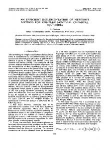
2 Decomposition I: Fluid – Structure The main idea behind the concept of partitioned fluid-structure simulations is simplicity and flexibility with respect to the choice of solvers and the coupling strategy. However, it is not trivial to reach this task in practice. Here, the development of appropriate software components for the coupling of two different codes is decisive but, in contrast to the examination of numerical coupling strategies, a somewhat neglected field. Thus, we will concentrate on these neglected informatical aspects and propose a concept that can be ‘filled’ with the suitable mathematical content in a flexible way. The most widely used software MpCCI works quite well for a fixed pair of codes but has severe drawbacks as soon as one wants to exchange solvers and/or the coupling strategy frequently. To eliminate these drawbacks, we introduce a client-server approach with a coupling client containing the coupling strategy and acting as a really separating layer between the solvers, which strongly facilitates the exchange of components of the coupled simulation. The coupling client has to address two components of coupling: first, the exchange of interface data (such as velocities, forces, . . .) between the solvers involved and, second, the control of the coupled simulation, that is the execution of the coupling strategy (explicit/implicit). Figure 2 displays the general concepts of MpCCI and of our approach [3].
2.1 Data Exchange At the interface between fluid and structure, we have to introduce some mapping of data between two, in general non-matching grids. In the MpCCI concept, this mapping is done directly from one solver to the other with the help of either given library routines or specialized user-defined interpolations. This implies that each solver has to know the grid of the other solver and, thus, inhibits the exchange of one solver without changing the code of the other one. Our concept introduces a third separate component, the coupling component, which holds its own description of the interface between fluid and structure in the form of a surface triangulation (Fig. 3), which we will refer to as the central mesh in the following. The solvers have to map their data
Efficient Implementation of DD for Fluid-Structure Interactions
Client
MPCCI interpolation ta da ta da
593
st ue req ta da
da t da a ta
surface coupling
req ue st da ta
fluid solver
structure solver
server fluid
server structure
+ coupling
+ coupling
+ interpolation
+ interpolation
Fig. 2. Schematic view of the general coupling concepts used in MpCCI (left) and in our framework (right).
to or get their data from the central mesh. Thus, we can now exchange one solver without changing the data mapping in the other one. Of course, the concrete choice of the resolution and the grid points of the central mesh may depend on one or both solver grids. However, the general concepts and algorithms needed in each solver to perform the mapping of data between the solver grids and the central mesh are not affected by this concrete choice as they only depend on the principle structure of the central mesh. The basis for all data mappings between solver grid and central mesh is – independent of the concrete choice of interpolation and projection operators – the identification of relations between data points of both grids. For the mapping of data from the solver to the central mesh, these relations are in general inclusion properties of surface nodes with respect to the solver grid cells. For the transport of data the way back from the central surface mesh to the solver grid, we need projections from the solver grid nodes to the surface triangles (see Fig. 3 for an example with a cartesian fluid grid). Whereas localizing a surface node in a solver grid cell is an easy task, finding projections on surface triangles requires more sophisticated methods. At this point, space-partitioning grids come into play as a key structure for the access of the (two-dimensional) surface triangulation in a spatial (three-dimensional) context. *!) *!) *) %!&!%!&!%!&!%!&!%!&!%!&!%!&!%!&!%!&!%!&!%!&!%!&!%!&!%!&!%& *!)) *!)) *)) &!%!%!&!%!%!&!%!%!&!%!%!&!%!%!&!%!%!&!%!%!&!%!%!&!%!%!&!%!%!&!%!%!&!%!%!&!%!%!&!%!%!&%% *#!*!# *# '&!% '&!% '&!% '&!% '&!% '&!% '&!% '&!% '&!% '&!% '&!% '&!% '&!% '&!% '&% $!*!)$#!$#!$!*!#)$!$!# $*#)$$# (!'&!(!(!' (!'&!(!(!' (!'&!(!(!' (!'&!(!(!' (!'&!(!(!' (!'&!(!(!' (!'&!(!(!' (!'&!(!(!' (!'&!(!(!' (!'&!(!(!' (!'&!(!(!' (!'&!(!(!' (!'&!(!(!' (!'&!(!(!' (('&(' $!#$!# $!#$!# $#$# (!'(!' (!'(!' (!'(!' (!'(!' (!'(!' (!'(!' (!'(!' (!'(!' (!'(!' (!'(!' (!'(!' (!'(!' (!'(!' (!'(!' ('(' $#!$!# $!#$!# $#$# (!'(!' (!'(!' (!'(!' (!'(!' (!'(!' (!'(!' (!'(!' (!'(!' (!'(!' (!'(!' (!'(!' (!'(!' (!'(!' (!'(!' ('(' $$#!!# $!$!## $$## (!(!'' (!(!'' (!(!'' (!(!'' (!(!'' (!(!'' (!(!'' (!(!'' (!(!'' (!(!'' (!(!'' (!(!'' (!(!'' (!(!'' (('' # # #' ' ' ' ' ' ' ' ' ' ' ' ' ' ' $!$!#$#!$!$!#$!# $$#$# (!(!'(!' (!(!'(!' (!(!'(!' (!(!'(!' (!(!'(!' (!(!'(!' (!(!'(!' (!(!'(!' (!(!'(!' (!(!'(!' (!(!'(!' (!(!'(!' (!(!'(!' (!(!'(!' (('(' $!#$!# $!#$!# $#$# (!'(!' (!'(!' (!'(!' (!'(!' (!'(!' (!'(!' (!'(!' (!'(!' (!'(!' (!'(!' (!'(!' (!'(!' (!'(!' (!'(!' ('(' $#!$!# $!#$!# $#$# (!'(!' (!'(!' (!'(!' (!'(!' (!'(!' (!'(!' (!'(!' (!'(!' (!'(!' (!'(!' (!'(!' (!'(!' (!'(!' (!'(!' ('(' "!"!"!"!"" "!"!"!"!"!"!""" "!"!"!"!"" "!"!"!"!"" "!"!"!"!"" "!"!"!"!"" ""!!"!"!""
Fig. 3. Left: Surface triangulation of a cylinder and cartesian grid cells at the boundary of the cylinder; right: data transport between the surface triangulation and a cartesian fluid grid: interpolation of stresses at surface nodes from values at the nodes of the fluid grid cell containing the respective surface node (left), copying data from projection points of fluid boundary points on the surface triangulation to the respective boundary grid point (right, taken from [3]).
594
M. Mehl, T. Neckel, T. Weinzierl
The algorithm to determine projection points is very closely related to the algorithm creating a new space-partitioning fluid grid (see Sect. 3) from the surface triangulation. In both cases, we have to identify intersections of solver grid cells and surface triangles. Here, the big potentials of space-partitioning grids are their inherent location awareness and their recursive structure, which permits the development of highly efficient algorithms exploiting the possibilities of handing down informations already gained in father cells to their son cells. Figure 4 gives an impression on how fast the resulting algorithms work for the example of grid generation.
octree depth time (in sec.) # octree nodes 7 0.872 84, 609 9 3.375 1, 376, 753 11 24.563 22, 104, 017 13 293.875 353, 685, 761
Fig. 4. Runtimes for the generation of an octree grid from a surface triangulation of a car. Computed on a Pentium 4 with 2.4GHz and 512kB Cache and sufficient main memory to hold all data required (Intel C++ compiler 8.0).
2.2 Coupling Strategy Except from data transfer, all other aspects of the coupling of two codes such as the definition and implementation of a coupling strategy and control of the whole coupled simulation are left to the user in MpCCI. That is, they have to be implemented in one or both of the involved solvers. As a consequence, an independent exchange of on component, either the coupling strategy or one of the solvers, is impossible. In contrast, our concept is based on a client-server approach (Fig. 2 and [2]). A socalled coupling-client controls the whole simulation. Fluid and structure solvers act as servers receiving requests from the client. The coupling strategy is implemented in the client and, thus, separated from the solvers.
3 Parallel Fluid Solver This paragraph describes some properties and aspects of our fluid solver currently being developed [3]. Hereby, the focus is to provide a solver which at the same time offers the possibility to exploit the most efficient numerical methods such as multigrid and grid adaptivity and, at the same time, to be highly efficient in terms of hardware or, in particular, memory usage and parallelizability. In this paper,
Efficient Implementation of DD for Fluid-Structure Interactions
595
we restrict ourselves to the parallelization concepts which again are, the same as all other technical and implementation aspects, independent on the concrete mathematical content (FE-/FV-discretization, linear/nonlinear solvers, etc.). The only invariant is the choice of cartesian space-partitioning grids as computational grids. These grids offer several advantages. First, their strict structure minimizes memory requirements. Second, the recursive structure allows for a very cache-efficient implementation of data structure and data access (see [6]). Third, grid adaptivity can be arbitrarily local (no restriction to block-adaptivity). Fourth, the mapping of data between the solver grid and the central mesh of the coupling client is supported in an optimal way as the mapping algorithms are based on space-partitioning cartesian grids themselves (cf. Sect. 2.1 and Fig. 4). Fifth, finally, a balanced parallelization can be done in a natural way using the properties of space-filling curves. Figure 5 shows a cut-off of the computed flow field together with the underlying grid for the two-dimensional flow around a cylinder at Reynolds number 20.
Fig. 5. Flow around a cylinder (Reynolds number 20): cut-off of the flow field and the underlying grid. For the parallelization of our flow solver, we developed an implementation of a spatial domain decomposition method based on the combination of our spacepartitioning computational grid with space-filling curves, which are known to be an efficient tool for the parallelization of algorithms on adaptively refined grids [5]. Hereby, the ‘obvious’ method is to string together the cells of the adaptive grid along the corresponding iterate of a space-filling curve and afterwards ‘cut’ the resulting cell string into equal pieces and assign one process to each of the pieces. For the domains of the single processes formed by these pieces of the cell string, a quasi-minimality of the domain surface resulting from the locality properties of the space-filling curve can be shown [5]. Thus, we get a balanced domain decomposition with quasi-minimal communication costs. The disadvantage of this simple approach is that we have to process the whole grid sequentially to build up the cell string. In contrast to this, our domain decomposition algorithm works completely in parallel. It never has to handle the whole grid on a single master processor. Instead, we recursively distribute sub-tree of the cell-tree among the available processors simultaneously to the set-up phase of the adaptive grid. Each process refines its domain until it reaches a limit in the work load that requires the outsourcing of sub-
596
M. Mehl, T. Neckel, T. Weinzierl
trees to other processes. Thus, every process holds a complete space-partitioning grid and all the distributed space-partitioning grids together form the global grid or the associated tree, respectively (see Fig. 6). Note that this level-wise domain decomposition process implies a tree order of the computing nodes, too. In the end, the algorithm lists the nodes level by level depending on the workload and, thus, the algorithm is pretty flexible concerning dynamical self-adaptivity. To maintain a balanced load distribution even for extremely local adaptive grid refinements (e.g., at singularities) and grid coarsenings (e.g., as a reaction to changing geometries), the algorithm also supports the merging of the grid partitions of two processes.
Fig. 6. Distribution of a space-partitioning grid (left) and the associated tree (right) to four processes (marked black, dark grey, grey and white). Our algorithm uses the Peano space-filling curve to traverse the grid cells and, thus, also splits up the domain at certain points on this curve. As mentioned above, the resulting partition is known to be quasi-optimal and connected [5]. In addition to producing a quasi-minimal amount of communication, the Peano curve allows for a very efficient realization of the communication due to two properties (e.g., which we could not show for any Hilbert curve). First, the Peano curve fulfills a projection property [7], that is the d-dimensional mapping onto a lower-dimensional submanifold aligned with the coordinate axes results in a lowerdimensional Peano curve. Second, it has the so-called palindrome property [7], that is the processing order of cell faces on such a submanifold is not only a Peano curve again but even the same Peano curve at both sides of the submanifold only with inverted order. Thus, the locality properties of the Peano curve on a submanifold separating two partitions imply good data access locality in the interprocess communication and, in addition, due to the palindrome property, there is no need for reordering data sent to neighboring processes. This highly improves the communication efficiency. In Table 1, we give some results achieved with an old version of our program still relying on a sequential domain decomposition algorithm and not yet working with asynchronous communication as our new code does. The left picture of Fig. 1 shows the domain decomposition for an adaptive two-dimensional grid for a sphere computed with our new code.
4 Conclusion We proposed concepts for two substantially different types of domain decomposition occurring in the context of partitioned simulation of fluid-structure interactions. We
Efficient Implementation of DD for Fluid-Structure Interactions
597
Table 1. Parallel speedup achieved for the solution of the three-dimensional Poisson equation on a spherical domain on an adaptive grid with 23, 118, 848 degrees of freedom. The computations were performed on a myrinet cluster consisting of eight dual Pentium III processors with 2 GByte RAM per node [8]. processes 1 2 4 8 16 speedup 1.00 1.95 3.73 6.85 12.93
could show the great potential of space-partitioning grids in each case. For the linkup of fluid and structure solver via a coupling client we use them as a tool to develop fast algorithms to connect the different grids involved. In the fluid solver itself, they are used as a computational grid, enhancing (among others) the parallelization possibilities. With this work, we have shown the general functionality and efficiency of all components: octree algorithms in the coupling client, Navier-Stokes solver on adaptively refined Cartesian grids, balanced parallelization of a solver on adaptively refined Cartesian grids. From this basis, we will establish a unified framework for the simulation of fluid-structure interactions including a (commercial) structure solver, integrate different mathematical methods for code coupling, data mapping, discretization, and linear solvers and perform numerous simulations for various examples to further approve the payload and the flexible applicability of our basic concepts.
References [1] U. Becker-Lemgau, M. Hackenberg, B. Steckel, and R. Tilch. Interpolation management in the grissli coupling-interface for multidisciplinary simulations. In K.D. Papailiou, D. Tsahalis, J. P´eriaux, C. Hirsch, and M. Pandolfi, editors, Computational Fluid Dynamics ’98, Proceedings of the 4th Eccomas Conference 1998, pages 1266–1271, 1998. [2] M. Brenk, H.-J. Bungartz, M. Mehl, R.-P. Mundani, A. D¨ uster, and D. Scholz. Efficient interface treatment for fluid-structure interaction on cartesian grids. In Proc. of the ECCOMAS Thematic Conf. on Comp. Methods for Coupled Problems in Science and Engineering, 2005. [3] M. Brenk, H.-J. Bungartz, M. Mehl, and T. Neckel. Fluid-structure interaction on cartesian grids: Flow simulation and coupling environment. In H.-J. Bungartz and M. Sch¨ afer, editors, Fluid-Structure Interaction, volume 53 of Lecture Notes in Computational Science and Engineering, pages 233–269. Springer, 2006. [4] H.-J. Bungartz and M. Mehl. Cartesian discretisation for fluid-structure interaction - efficient flow solver. In Proceedings ECCOMAS CFD 2006, European Conference on Computational Fluid Dynamics, Egmond an Zee, September 5th8th 2006, 2006. [5] M. Griebel and G.W. Zumbusch. Hash based adaptive parallel multilevel methods with space-filling curves. NIC Series, 9:479–492, 2002.
598
M. Mehl, T. Neckel, T. Weinzierl
[6] F. G¨ unther, M. Mehl, M. P¨ ogl, and Ch. Zenger. A cache-aware algorithm for pdes on hierarchical data structures based on space-filling curves. SIAM J. Sci. Comput., 28(5):1634–1650, 2006. [7] A. Krahnke. Adaptive Verfahren h¨ oherer Ordnung auf cache-optimalen Datenstrukturen f¨ ur dreidimensionale Probleme. PhD thesis, Institut f¨ ur Informatik, TU M¨ unchen, 2005. [8] M. Mehl. Cache-optimal data-structures for hierarchical methods on adaptively refined space-partitioning grids. In M. Gerndt and D. Kranzlm¨ uller, editors, International Conference on High Performance Computing and Communications 2006, HPCC06, volume 4208 of LNCS, pages 138–147. Springer, 2006. [9] Fraunhofer SCAI. Mpcci: Multidisciplinary simulations through code coupling, version 3.0.4 MpCCI Manuals [online], url: http://www.scai.fraunhofer.de/592.0.html [cited 18 oct. 2006], 2006.