Conceptual basis and spatial modelling to account for and conserve ...

Conceptual basis and spatial modelling to account for and conserve multiple ecosystem services in Telemark County, Norway

Matthias Schröter

Thesis committee Promotors Prof. Dr H.B.J. Leemans Professor of Environmental Systems Analysis Wageningen University Prof. Dr L.G. Hein Personal chair at the Environmental Systems Analysis Group Wageningen University Co-promotor Dr D.N. Barton Senior Researcher NINA – Norwegian Institute for Nature Research, Oslo Other members Prof. Dr A.K. Bregt, Wageningen University Prof. Dr P.H. Verburg, VU University Amsterdam Dr B. Burkhard, University of Kiel, Germany Dr I. Aslaksen, SSB – Statistics Norway, Oslo, Norway

This research was conducted under the auspices of the Graduate School for SocioEconomic and Natural Sciences of the Environment (SENSE).

Conceptual basis and spatial modelling to account for and conserve multiple ecosystem services in Telemark County, Norway

Matthias Schröter

Thesis submitted in fulfilment of the requirements for the degree of doctor at Wageningen University by the authority of the Academic Board, in the presence of the Thesis Committee appointed by the Academic Board to be defended in public on Wednesday 10 June 2015 at 11 a.m. in the Aula.

Matthias Schröter Conceptual basis and spatial modelling to account for and conserve multiple ecosystem services in Telemark County, Norway, 197 pages. PhD thesis, Wageningen University, Wageningen, NL (2015) With references, with summaries in English and Dutch ISBN 978-94-6257-312-3

Acknowledgements Only one name shows on the cover of this book, but writing this thesis would have been impossible without the support of many people, among others, my promotors, co-promotor, co-authors, funders, colleagues, housemates, friends, family and my partner. I gratefully acknowledge funding of my studies by the European Research Council (grant 263027, “Ecospace” project). I furthermore acknowledge financial support of the Research Council of Norway for the Yggdrasil research stay at the Norwegian Institute for Nature Research in Oslo. I also acknowledge financial support from the Environmental Systems Analysis group at Wageningen University. I thank Rik Leemans for accepting me as a PhD candidate at his chair group. Rik, your feedback has been challenging, sharp, direct and always very constructive. I also enjoyed inspiring debates about society and the deeper meaning behind science. When I was challenged putting my work together, you kindly pointed to Kierkegaard, who said that life is to be lived forward, and reviewed backwards. I thank Lars Hein for offering me the opportunity to start a PhD in his research project. When you switched to Norwegian in the job interview, I knew that this was the challenge I was searching for. Lars, you have taught me how to be the most critical reviewer of myself. I acknowledge your constant feedback. A big thank also goes to David Barton for agreeing to be my co-supervisor and copromotor. David, I particularly enjoyed discussing the policy-relevance of my work. Your compliments often came when I needed them the most. I remember well your “kompis” joke in San José. During my time as a PhD candidate, I had the pleasure to conceptualise, design and perform several paper-based projects with great people from different countries and with different backgrounds. They inspiringly discussed and provided feedback on many issues and explored the power of good cooperation. I had the pleasure to work in different languages with you, so I would like to say “Hartstikke bedankt” to Roy, Lars, Emma, Alexander, Paul, Dolf and Bram. “Tusen takk” to David, and “Tusen tack” to Graciela and Björn. “Vielen Dank” Stefan, for your GIS help and advice, and, finally, “Thanks” to Hector, Carl and Elham. I thank Wageningen University and its staff for offering an inspiring, motivating and highly professional academic surrounding. I thank NINA, and in particular Erik Framstad and Henrik Lindhjem for inviting me to come to Oslo and work in a different scientific and physical environment. Many thanks to my dear colleagues at the Environmental Systems Analysis group at Wageningen University! Thank you, Dolf, for introducing me to the ESP network and for giving me the chance to work for the International Journal of i

Biodiversity Science, Ecosystem Services and Management. I very much enjoyed developing the journal together with Alexander and you, and seeing it grow. Thanks for all the trust you put in us. I thank Karen for nice discussions about interdisciplinarity and education, and for letting me be part of the supervision team of the essay writing course. Thank you, Mathilde, for your valuable support, in particular with printing the thesis when I already moved to Germany. Thanks to the senior staff at ESA, Arnold, Wichertje, Bas, Nynke, Carolien, Wim and André, for nice and friendly conversations. My PhD fellows at ESA made the four years in the Netherlands four very special ones. Thanks first and foremost to my closest colleagues and roommates Roy and Aritta. No matter what challenges we had to face during the PhD, we stood together and helped each other wherever possible. Thank you, Roy for reminding me of the life outside the office, your positive attitude and your support with my work. I very much enjoyed brainstorming and exchange on the contents of our theses. I remember well leaving our office to go to idyllic Peyresq, experiencing our first international conference in Kiel, eating vegan burgers in Berlin and discovering San José and surroundings. Aritta, I enjoyed discussions about our topics, giving and receiving feedback and also sharing private stuff. Dining at your place and enjoying your excellent food was a very special experience. I appreciate your infinite friendliness and trust. Thanks to Alexander for sharing thoughts about the university, life and all the rest. Thanks for brainstorming, working late and an unforgettable cooperation on the ‘contested’ article project. Your passion for both science and word jokes formed a perfect synergy. I enjoyed being part of the ever growing PhD group at ESA, including Alexander, Roy, Clara, Ingeborg, Lucie, Lena, Anne, Sander, Martine, Aritta, Sara and Linda. Hiking is probably one of the nicest forms of moving from A to B (only 2nd on the list are train rides between Wageningen and Oslo). I liked to hike with you to discover the campus during lunch breaks and having dinners and beers after work Thanks to Lena, for critical remarks on my introduction and critical discussions in general. Thanks to Clara, for sharing a remarkable international conference experience and for discovering the surroundings of the conference location. Thank you, Sander, for nice, friendly and helpful discussions on the process of writing a PhD. Thank you Lucie and Ingeborg for critically reading my introduction and chapters. I enjoyed your company a lot. Thanks to my other PhD colleagues Cheng, Katalin, Elham, Leonardo, Confidence, Eugenie and Maryna for nice and constructive discussions. Thanks to all those who shared a house with me during my PhD (I counted 17!). My homes and homies in the fabulous “Boerderie” in the Binnenveld, in Nijmegen and Ede created a valuable balance to the sometimes stressful research. Thanks in ii

particular to Emma, Kimo and Djai, who made their home mine. Thanks also to the Wageningen Athletic Club Tartlétos, all my running mates on the blue track and the fabulous coach Tonnie Dirks. Running in company at the end of a working day has always provided a welcome distraction from the work on this thesis. My friends and family have not seen me or heard much of me at times when I dived into my work. Thanks to all of you for your patience, your sympathy and understanding. Thank you, Timo, for the extraordinary time we shared in Wageningen. I know I can steal horses with you - and hug them, if the situation allows. Your support was strong when I needed it the most. Thank you, Jacqui, for exchanging thoughts on our common journey through the world of science. It has been a long journey from our first shared day at the university to the defences of our theses and I am happy to have you at my side. Thanks also for reading and commenting on introduction and conclusion. Thank you, Alexandra, for listening and your immense care. Thanks to Marie, Til and Karin for continuously daring to ask how my PhD is proceeding. I thank my sister Marit for her patience and support. I am glad to have a mother that supported me in whatever I chose to do in my life. This book could be written because you were there, always believing in me, with an enormous interest in what your son is doing. Vielen Dank, Mutti. My last thanks go to you, Paulien, for your amazing capacity of understanding what I am thinking, your wonderful intuition of what was going on during my PhD and in my mind. Your wise and sometimes unconventional advice enormously helped in finding solutions.

iii

Table of Contents 1

Introduction: challenges in conceptually framing, spatially assessing and

conserving ecosystem services .......................................................................................... 1 2

Ecosystem services as a contested concept: a synthesis of critique and counter-

arguments .......................................................................................................................... 15 3

Accounting for capacity and flow of ecosystem services: A conceptual model

and a case study for Telemark, Norway ........................................................................ 33 4

Spatial prioritisation for conserving ecosystem services: a comparison of

hotspot methods with a heuristic optimisation approach .......................................... 69 5

Integrating ecosystem services into site prioritisation for conserving forest

biodiversity ........................................................................................................................ 97 6

Synthesis, discussion and conclusion .................................................................. 123

References ........................................................................................................................ 139 Appendix I ....................................................................................................................... 159 Appendix II ...................................................................................................................... 164 Appendix III .................................................................................................................... 165 Appendix IV .................................................................................................................... 173 Appendix V ..................................................................................................................... 175 Appendix VI .................................................................................................................... 176 Appendix VII ................................................................................................................... 177 Appendix VIII ................................................................................................................. 178 Appendix IX .................................................................................................................... 179 Appendix X ...................................................................................................................... 180 Summary .......................................................................................................................... 182 Nederlandstalige samenvatting .................................................................................... 187

Introduction

1

Introduction: challenges in conceptually framing, spatially assessing and conserving ecosystem services

Partly based on: Schröter, M., Remme, R.P., Hein, L., 2012. How and where to map supply and demand of ecosystem services for policy-relevant outcomes? Ecological Indicators 23, 220-221. Schröter, M., Remme, R.P., Sumarga, E., Barton, D.N., Hein, L., 2015. Lessons learned for spatial modelling of ecosystem services in support of ecosystem accounting. Ecosystem Services. In press.

1

Chapter 1

1.1 Background Ecosystem services (ESs) are increasingly being used as an approach to analyse the relationship between humans and nature (Carpenter et al., 2009; Fisher et al., 2009). Humans benefit from ecosystems in several ways (de Groot et al., 2002; HainesYoung and Potschin, 2013). Ecosystems contribute to human well-being by providing resources, creating benign environmental conditions and offering the potential for socio-cultural fulfilment (Wallace, 2007). For instance, ecosystems provide food, construction material and fuel (i.e. provisioning services). Ecosystems regulate environmental flows in a beneficial way, such as carbon sequestration, and erosion prevention (i.e. regulating services). Furthermore, ecosystems provide opportunities for intellectual and spiritual interactions with nature, such as possibilities for recreation and aesthetic enjoyment (i.e. cultural services). The awareness that humans depend on ecosystems and their services is much older than the scientific analysis of ESs. Plato and Aristotle, for example, related deforestation and soil erosion in ancient Greece (Runnels, 1995). The ES concept also has a long history within environmental sciences (Gómez-Baggethun et al., 2010). Early notions of the concept can, for example, be traced to Hueting (1970, p. 65), who pointed out that “measuring the value of nature has to start with an exhaustive listing of the functions that nature has for mankind” (own translation from Dutch). Westman (1977, p. 960) illustrated the “importance of accounting for the benefits of nature's ‘services’”, and Ehrlich and Ehrlich (1981, p. 6) argued that fighting species extinction should take place not only, but also because of the “indispensable free services” that ecosystems provide. The ES concept became mainstream in scientific literature in the 1990s (Costanza et al., 1997; Daily, 1997; de Groot, 1992), and in the early 2000s the concept was increasingly put on the political agenda. The Millennium Ecosystem Assessment (MA, 2005) and The Economics of Ecosystems and Biodiversity (TEEB; Kumar, 2010) provided important results and drivers to increase scientific interest in ESs. While the search term “ecosystem service*” appeared in only 66 studies published throughout 1997, this number had risen to 440 in 2005 and over 2750 in 2013 (based on a Scopus search on 21 November 2014). Despite the considerable amount of research on ESs and the increasing number of studies that apply the concept, different interpretations of the concept still cause 2

Introduction

confusion (Boyd and Banzhaf, 2007; Nahlik et al., 2012). In this thesis, ESs are defined as “the contributions that ecosystems make to human well-being, and [that]

arise

from

the

interaction

of

biotic

and

abiotic

processes

[in

ecosystems]”(Haines-Young and Potschin, 2010b, p. i). Contributions are those properties of an ecosystem that are beneficial for humans (e.g. certain population sizes, regrowth rates, certain ecosystem states). Properties result from ecosystem processes, which include transfers of energy, matter and information. The term ‘contributions’ indicates that next to ecosystem contributions often also human contributions are needed to create benefits for humans. The final use of many ESs only takes place after economic actors (e.g. ecosystem managers, primary resource exploiters, private persons) have modified ecosystems, harvested or actively used services. This is in particular the case for many provisioning services. Management to create access to ecosystems and activities of humans who benefit from services are also needed for realisation of many cultural ESs (Remme et al., 2014). As a consequence, ESs need to be conceptualised and analysed at the interface between ecosystems and society. ES can be used as an anthropocentric argument for both protection and for sustainable management of ecosystems (Jax et al., 2013; Lamarque et al., 2011a; Reid et al., 2006). The ES concept has recently been adopted by several international

initiatives

at

the

science-policy

interface,

such

as

the

Intergovernmental Platform on Biodiversity and Ecosystem Services (IPBES, Larigauderie and Mooney, 2010) and the System of Environmental-Economic Accounting (SEEA) Experimental Ecosystem Accounting guidelines (European Commission et al., 2013). Those initiatives are accompanied by calls for further operationalization of the ES concept for decision making (Daily et al., 2009). Among others, systematic assessment and monitoring of ESs (Carpenter et al., 2009; Larigauderie et al., 2012) and integration of ESs into planning (Albert et al., 2014; Cowling et al., 2008) are needed. Such planning can refer to both sustainable use of multiple ESs (Brussard et al., 1998; de Groot et al., 2010a; Fisher et al., 2009) and protection of the natural environment (Cimon-Morin et al., 2013; Egoh et al., 2007). However, it is a long way from the simple notion that ecosystems provide essential services, to the spatially explicit measurement of ESs and implementation of the ES concept in decision-making. For further operationalization of the ES concept for decision-making several challenges need to be addressed. Some of 3

Chapter 1

these issues are outlined below and they form the basis for the formulation of the research objectives of this thesis. 1.2 Addressing multifaceted critique on the ecosystem service concept In order to operationalize the ES concept and to successfully implement ESs in decision-making on sustainable use and protection of ecosystems, one needs to carefully investigate the controversy around the concept, which has risen in the last decade (e.g., Barnaud and Antona, 2014; McCauley, 2006; Redford and Adams, 2009). The ES concept is a normative concept (i.e. a value-based idea of how environmental problems should be addressed). The use of normative concepts, is characteristic for environmental sciences, where a cognitive interest is often combined with an action interest (Baumgärtner et al., 2008). The ES concept has its roots in an anthropocentric worldview to manage ecosystems and biodiversity in particular in areas outside protected areas (Reid et al., 2006). Here, arguments for sustainable use or protection of biodiversity and ecosystems are based on their instrumental value for humans (Jax et al., 2013; Justus et al., 2009). There is a debate whether arguments for conservation should be based on such anthropocentric values or on inherent or intrinsic values, which exist regardless of a valuing human being (Jax et al., 2013; Justus et al., 2009). The intrinsic value argument is often used for biodiversity protection (Maguire and Justus, 2008). The long-standing ethical debate on anthropocentric versus intrinsic values for conservation and sustainable use of ecosystems is one of the most important controversies around the ES concept. The controversy around the ES concept might stem from its role as a transdisciplinary boundary object (Abson et al., 2014). Scientists from different disciplines with different paradigms work with the same concept. For instance, ecologists are often sceptical towards the ES concept and often view people as an “ecological audience” (Lowe et al., 2009). Economists, on the other hand, are often attracted by the anthropocentric, utilitarian framing of the concept (Luck et al., 2012a). Nuances in between these positions exist, of course, and belonging to a certain discipline as such is not an indicator for disagreement to promotion of the ES concept. In the course of the controversial debate about ESs, however, a couple of misleadingly narrow interpretations of the ES concept have recently appeared in the literature. For instance, the use of the ES concept for conservation is seen as 4

Introduction

“selling out on nature” (McCauley, 2006) or as a “technocratic and economic perspective” (Turnhout et al., 2013). Such interpretations need to be clarified and addressed, as contestation of the conceptual basis of subsequent ES assessments and applications might reduce their acceptance in decision making (Justus et al., 2009). 1.3 Capturing spatial heterogeneity of capacity and flow of ecosystem services ESs have a spatial dimension. The locations of ecosystems and beneficiaries are crucial elements to consider in ES assessments (Boyd, 2008; Costanza, 2008). Ecosystems can provide ESs to beneficiaries in the same area, as well as in surrounding (Fisher et al., 2009) and distant areas (Hein et al., 2006). This provision of a service can be directional, such as people benefitting from upstream flood regulation (Nedkov and Burkhard, 2012), or omnidirectional such as pollination or carbon sequestration (Serna-Chavez et al., 2014). Geographic analysis of ESs is thus at the basis of operationalization for decision-making (Boyd, 2008). ESs are not distributed equally across an area but show spatial heterogeneity. Heterogeneity is defined here as the degree of variation within the spatial distribution of an ES. Important factors that determine heterogeneity include ecosystem diversity, variation of environmental conditions (e.g. slope, climate and soil conditions), land management, and inter-site linkages of environmental flows. Another important factor that increases ES heterogeneity is movement of service providing units (e.g. animal populations for hunting; Luck et al., 2009). Beneficiaries of ESs add spatial variation through use patterns that differ across space. For example, beneficiaries move across landscapes and their preference vary, which leads to spatially heterogeneous patterns of ESs (Costanza, 2008). Many studies recognised the need for spatially explicit assessments of ESs (Seppelt et al., 2011) and also the recent Ecosystem Accounting guidelines emphasised the need for a geographic analysis of ESs (European Commission et al., 2013). An immense variety of methods has been developed to model multiple ESs at different spatial scales (Crossman et al., 2013; Maes et al., 2012a; Martínez-Harms and Balvanera, 2012). The results of such spatial models are maps, which can be defined as simplified representations of reality. In other words, “a map is not the territory” (Korzybski, 1996, p. 750). Spatial modelling of ESs strives for accuracy. Accuracy refers to the degree of correspondence between spatial modelling results 5

Chapter 1

and the modelled object or phenomenon (Harvey, 2008). Accuracy indicates how well a spatial model estimates the real distribution and abundance of an ES at a resolution, which is high enough to cover the phenomena of interest. Although there are many spatial ES assessment studies, only a few have spatially assessed different components of ESs (Burkhard et al., 2012; Nedkov and Burkhard, 2012; Petz and van Oudenhoven, 2012; van Jaarsveld et al., 2005). ES components can be understood as elements of ecosystems and of humanecosystem-interactions that are essential for the provision of a service. Due to restrictions such as low spatial accessibility, which leads to absence of beneficiaries, not all ecosystem properties constitute an ES. The potential provision and the actual use of ESs should be distinguished as different components of ESs. This has been widely acknowledged (De Groot et al., 2010b; Haines-Young and Potschin, 2010a; van Oudenhoven et al., 2012), but some confusion has arisen in the use of terms for these components. A recent integrative review of these terms suggests that ‘capacity’ is the potential of ecosystems to provide services and ‘flow’ is the actual use of services (Villamagna et al., 2013). These definitions are in line with definitions for capacity and flow in this thesis. Clarity of terms and definitions is one crucial aspect also for locating components of ESs. Another important challenge is to develop compatible indicators for capacity and flow as well as decision rules for localising capacity and flow on a map (Burkhard et al., 2014). Increasing conceptual clarity, finding appropriate indicators and developing methods to spatially assess ESs is essential in advancing ecosystem accounting as well as policy applications that built on spatial ES information. 1.4 Incorporating spatial relations between multiple ecosystem services and between ecosystem services and biodiversity into site prioritisation for conservation Calls for considering ESs in decision-making originated from a concern about the state of the natural environment and biodiversity in particular. Applying the ES concept for conservation purposes, however, is a fairly new practice and the ES concept still needs to be operationalized (Chan et al., 2011; Cimon-Morin et al., 2013; Egoh et al., 2007). Conservation has been framed to address the loss of biodiversity, often for its own sake, but at the same time recognising human presence in ecosystems as well as human needs (Callicott, 2006; Meffe et al., 2006). 6

Introduction

Conservation is understood in this thesis, sensu World Resources Institute et al. (1992, p. 228), as an umbrella term for different forms of sustainable ecosystem management. Sustainable ecosystem management can be defined as human activities that maintain a long-term provision of ESs while staying within ecological limits (Brussard et al., 1998). This broad definition of conservation includes, inter alia, different degrees of ecosystem protection and sustainable ecosystem use (Redford and Richter, 1999; World Resources Institute et al., 1992). At least three challenges for operationalizing ESs in the context of conservation exist. I summarize them in the following sections. A first challenge is to distinguish services that are compatible with conservation from those that are incompatible (Chan et al., 2011). The development of the ES concept has led to extensive lists of ESs that are potentially provided by ecosystems (de Groot et al., 2002; Haines-Young and Potschin, 2013). These lists as well as spatial ES assessments have included provisioning services, which require relatively large human interventions during management and extraction of the service. Examples of such provisioning ESs that have been included in spatial assessments, include timber harvest and intensive agricultural and livestock production (Maes et al., 2012b; Raudsepp-Hearne et al., 2010; Rodríguez-Loinaz et al., 2015). Extracting such provisioning services can have severe negative effects on ecosystems, resulting in trade-offs with other ESs and biodiversity (Cimon-Morin et al., 2013). ESs are compatible with conservation if their occurrence in an area could reasonably be taken into account as an argument for conservation, and conservation would not restrict their use. This is the case for many regulating services (Egoh et al., 2009) and many cultural services (Daniel et al., 2012). Many provisioning services, however, would be restricted to some extent in protected areas. A second challenge is to incorporate spatial relations between services in prioritising sites for conservation. As conservation causes costs (Naidoo et al., 2006) and societal resources for conservation are limited, conservation planners need to prioritise sites for applying particular conservation policy instruments (Barton et al., 2013), such as delineation of new protected areas. Complexity in spatial relations between ESs can arise from the presence and state of different types of ecosystems. This can also be a result of impacts of common anthropogenic drivers or interactions between ESs, which can have positive or negative effects on 7

Chapter 1

specific ESs (Bennett et al., 2009). An example for such an interaction between ESs is the negative effect of timber harvest on carbon storage (Duncker et al., 2012). In order to analyse spatial relations between ESs, several studies have assessed pairwise correlations and proportional overlaps between different sets of ESs. Strength and direction of correlations between regulating and cultural services, which could potentially be considered in conservation, differed strongly between study areas and services, and ranged from medium negative to high positive correlations (Bai et al., 2011; Chan et al., 2006; Egoh et al., 2008; Jopke et al., 2015; Naidoo et al., 2008; Raudsepp-Hearne et al., 2010). Studies have also shown that the overlap between the distribution of different ESs differs strongly between study and areas services (Chan et al., 2006; Egoh et al., 2008; Wu et al., 2013). Such differences in spatial distribution heterogeneity need to be considered in site prioritisation for conservation. A third challenge is to integrate both biodiversity and ESs into conservation planning. There has been a debate on how the concepts of biodiversity and ESs relate to each other (Adams, 2014; Mace et al., 2012; Reyers et al., 2012b). In principle, biodiversity can play a role either in regulating ecological processes, which contribute to final ESs (Balvanera et al., 2006; Cardinale et al., 2012; Harrison et al., 2014), or as a final ES, which could relate to appreciation of genetic diversity (e.g., different sorts of apples) or the existence of populations of wild animals (e.g., for bird watching) (Mace et al., 2012). However, still little is known about the ecology behind ESs (Balvanera et al., 2014; Cardinale et al., 2012). Hence, many studies have considered spatial information on biodiversity in addition to spatial information on ESs to analyse spatial congruence and to adequately account for biodiversity (Cimon-Morin et al., 2013; Egoh et al., 2009; Maes et al., 2012b). Similarly, in this thesis biodiversity is not seen as an ES but included as a separate argument for conservation in the form of multiple biodiversity surrogates (vegetation types of high biodiversity value, old-growth forest structures etc.). A final challenge concerns the spatial distribution of conservation features. This is only one of several aspects that are necessary to consider within conservation planning (Margules and Pressey, 2000). Important other aspects involve target setting, which has seldom been done for ESs so far (Luck et al., 2012b), consideration of different opportunity costs per land unit (Naidoo et al., 2006) and compactness of protected sites (Possingham et al., 2006). Several studies have 8

Introduction

incorporated such a spatially explicit multi-criteria approach for conservation planning (Chan et al., 2011; Egoh et al., 2011; Izquierdo and Clark, 2012). However, how spatial priorities for conservation would change, if ESs were considered next to biodiversity aspects in conservation planning, is still unclear. 1.5 Objectives As has been outlined above, several challenges should be addressed in order to further operationalize the ES concept for accounting and systematic planning for conservation of biodiversity and ESs. The main objectives of this thesis are thus to explore and further develop the conceptual basis of ESs, and to create and apply spatial models of multiple ESs for accounting and conservation. These interdisciplinary objectives are addressed by critically reflecting on ESs, conceptual reasoning, methodological development of spatial modelling as well as applying the generated spatial models in hypothetical conservation scenarios. These objectives lead to the following research questions: 1.

What are the recurring critiques on the ES concept and what are their potential counter-arguments?

2.

How can both critiques and counter-arguments be used to advance the ES concept?

3.

How can an ecosystem’s capacity to provide ESs and the flow of multiple ESs be spatially and biophysically modelled for accounting?

4.

How can sites for ES conservation be prioritised by different methods?

5.

How can sites for biodiversity conservation be prioritised when ESs are included in systematic conservation planning?

Addressing these research questions will help to operationalize the ES concept for accounting and conservation in several ways. Reflecting on the critique on the ES concept and counter-arguments can help to improve the conceptual basis of the concept. Integrating critique on the ES concept and counter-arguments can help to formulate a way forward for the concept, which can facilitate and improve future applications. Furthermore, methodological progress in spatial modelling of both capacity and flow of ESs can help to create spatially explicit data to inform

9

Chapter 1

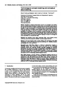
decision-making. Methodological development for integration of ESs into conservation as a potential field of application is subsequently demonstrated. To simplify complex systems for analysis is probably not preferable (Ostrom, 2007), albeit necessary to make complex systems analysable (Levins, 1966). This thesis takes a necessarily simplified, parsimonious top-down perspective on ecosystems, the ESs they provide and their conservation. A top-down perspective means that in this thesis I methodologically take the perspective of a planner, who monitors ESs for accounting and who searches for socially optimal solutions for conservation problems. The integration of the perspectives, values and individual decisions of autonomous actors as well as socio-economic and political dynamics, which in turn influence ecosystem dynamics, are considered beyond the scope of this thesis. In parts of this thesis (Chapters 3, 4 and 5) methods are applied to a case study in Telemark County, which is situated in southern Norway. The large size of the study area furthermore contributes to simplification of the analysis, as it uses a coarse grain for analysing services and does not consider heterogeneity between beneficiaries of services. As a consequence, the focus of this thesis is to scientifically explore potential methodologies for further operationalization of the ES concept, and results should not be interpreted as a concrete practical guidance for decision-making. 1.6 Study area Telemark (Figure 1.1) has an area of 15,300 km2 and a population of about 170,000 people living in 18 municipalities (SSB, 2012b). Population density varies from about 1 person per km2 in the west (Fyresdal) and north-west (Vinje) of the county to 65 (Skien) and 176 (Porsgrunn) in the south-east. The altitude ranges from sea level at the coast of the Skagerrak to 1883 m a.s.l. on the Gaustatoppen. The climate varies across the region with temperate conditions in the south-east (Skien, average temperature January -4.0 °C, July 16.0 °C, 855 mm annual precipitation) and alpine conditions in the north-west (Vinje, January -9.0 °C, July 11.0 °C, 1035 mm)

(Meteorological Institute, 2012a). Telemark stretches across five vegetation zones (boreonemoral, southern, middle, and northern boreal, alpine) (Moen, 1999). With its varied landscape types from fjords to the highland plateau, being representative for the country as a whole, Telemark has been termed “Norway in a miniature”.

10

Introduction

The southern part of Telemark is mainly covered by coniferous and boreal deciduous forest (Moen, 1999), which are exploited by humans for forestry activities. The southern part is also characterised by large inland lakes, with few towns and a small agricultural area (247 km2, about 1.6% of the land area) (SSB, 2012b). The northern part consists of treeless alpine highland plateaus covered by bogs, fens and heathlands (Moen, 1999). In 2011, 5.1% of the area of Telemark were protected in national parks, 4.6% in landscape protection areas (both types cover mainly highland plateaus), and 1.7% in nature reserves (SSB, 2012b). As a result of relative intensive forestry activities, biodiversity in forests of Telemark is relatively low compared to other ecosystems and regions within Norway (Certain et al., 2011).

Figure 1.1: Map of the study area. Data source: Norwegian Mapping authority, AR 50 dataset.

11

Chapter 1

1.7 Outline This thesis consists of six chapters (Fig. 1.2). Chapters 2 to 5 are conceptualised and written as independent scientific papers and can thus be read separately. In Chapter 2, seven recurring critiques of the ES concept and respective counterarguments are described and synthesized (research question 1). By disentangling and contrasting different arguments, a potential way forward for the ES concept is developed (research question 2). In Chapter 3, capacity and flow of nine ESs are conceptually distinguished and assessed for Telemark County. This is done by means of different spatial models, developed with various available datasets and methods, including (multiple layer) look-up tables, causal relations between datasets (including satellite images), environmental regression, and indicators derived from direct measurements. Conditions for a meaningful spatial capacity– flow-balance are discussed (research question 3). In a subsequent step (Chapter 4),

Figure 1.2: Outline of the thesis. Numbers in circles refer to chapters, numbers in brackets refer to research questions

12

Introduction

a selection of cultural and regulating ES flow maps is used to explore methods to prioritise areas for conservation of ESs. Methods to spatially delineate hotspots are reviewed and classified. The effect of different hotspot methods on spatial configuration of hotspots for this set of ecosystem services is tested. The outcomes are compared to a heuristic site prioritisation approach (Marxan) (research question 4). In Chapter 5, the same set of ESs is included in a conservation scenario for forest biodiversity with the help of the heuristic optimisation planning software Marxan with Zones. A mix of conservation instruments is combined, where timber harvest, an important provisioning services in Telemark, is either completely (nonuse zone) or partially restricted (partial use zone) (research question 5). Chapter 6 contains a general synthesis of the thesis, in which the methodologies and results are discussed.

13

Ecosystem services as a contested concept

2

Ecosystem services as a contested concept: a synthesis of critique and counter-arguments

We describe and reflect on seven recurring critiques of the concept of ecosystem services and respective counter-arguments. First, the concept is criticized for being anthropocentric, whereas others argue that it goes beyond instrumental values. Second, some argue that the concept promotes an exploitative human-nature relationship, whereas others state that it re-connects society to ecosystems, emphasizing humanity’s dependence on nature. Third, concerns exist that the concept may conflict with biodiversity conservation objectives, whereas others emphasize complementarity. Fourth, the concept is questioned because of its supposed focus on economic valuation, whereas others argue that ecosystem services science includes many values. Fifth, the concept is criticized for promoting commodification of nature, whereas others point out that most ecosystem services are not connected to market-based instruments. Sixth, vagueness of definitions and classifications are stated to be a weakness, whereas others argue that vagueness enhances transdisciplinary collaboration. Seventh, some criticize the normative nature of the concept, implying that all outcomes of ecosystem processes are desirable. The normative nature is indeed typical for the concept, but should not be problematic when acknowledged. By disentangling and contrasting different arguments we hope to contribute to a more structured debate between opponents and proponents of the ecosystem services concept.

Based on: Schröter, M., van der Zanden, E.H., van Oudenhoven, A.P.E., Remme, R.P., SernaChavez, H.M., de Groot, R.S., Opdam, P., 2014. Ecosystem services as a contested concept: a synthesis of critique and counter-arguments. Conservation Letters 7, 514523.

15

Chapter 2

2.1 Introduction The ecosystem services (ES) concept emphasizes the multiple benefits of ecosystems to humans (MA, 2005), and its use can facilitate collaboration between scientists, professionals, decision-makers, and other stakeholders. Although the concept has gained considerable interest in- and outside of science, it is increasingly contested and encounters multifaceted objections. We describe and reflect on seven critiques on the concept, summarize counter-arguments based on literature and inter-subjective deliberation, and propose a way forward. Rather than providing an exhaustive overview, we synthesize recurring critiques that were distilled from the rapidly expanding literature on ESs, discussions during conferences, and conversations with colleagues from different scientific disciplines. We selected three types of critical arguments against the concept. The first one covers ethical considerations, which relate to how humans interact with nature. We address critique regarding environmental ethics and regarding the human-naturerelationship. The second type of argument deals with strategies for nature conservation and sustainable use of ecosystems, which relate to the science-policy interface. These arguments include supposed conflicts with the concept of biodiversity, issues related to valuation, and commodification and Payments for Ecosystem Services (PES). The third type of argument is about the current state of ESs as a scientific approach. We discuss issues of vagueness of terms and definitions as well as optimistic assumptions and normative aims. 2.2 Critique and counter-arguments 2.2.1

Environmental ethics

2.2.1.1 Critique The ES concept is criticized for its anthropocentric focus and exclusion of the intrinsic value of different entities in nature (McCauley, 2006; Redford and Adams, 2009; Sagoff, 2008). This critique has its roots in a long-standing, unresolved debate within environmental ethics. This debate deals with the question whether our actions towards nature should be based on an anthropocentric view that constitutes instrumental values of nature, or whether they should be based on biocentric reasoning that constitutes intrinsic values of nature (Callicott, 2006; Jax et al., 2013; Krebs, 1999).

16


2.2.1.2 Counter-arguments a) The ecosystem service concept includes ethical arguments Jax et al. (2013) have pointed out that it is misleading to juxtapose an ethical position with the ES concept, as environmental ethics also includes anthropocentric values (Callicott, 2006; Krebs, 1999). In our world, where most ecosystems are managed, anthropocentric values provide additional arguments to address the ongoing ecological crisis (Reid et al., 2006; Skroch and López-Hoffman, 2010). The ES concept is not meant to replace biocentric arguments, but bundles a broad variety of anthropocentric arguments for protection and sustainable human use of ecosystems (Chan et al., 2012b; Luck et al., 2012a). Such arguments include ensuring the fulfilment of basic needs of current and future generations through provisioning, regulating and cultural ESs. b) The ecosystem service concept might allow for integration of intrinsic values Broad values, which contribute to a genuinely good life in an Aristotelian sense, go beyond considering nature as a toolbox for satisfying material needs (Krebs, 1999). For instance, aesthetic contemplation of an ecosystem requires the valued object to be valuable ‘in itself’, i.e. for its own purpose while at the same time being valued by a human being (Krebs, 1999). The cultural ES category shows overlaps between pure anthropocentric and intrinsic values. Certain forms of psycho-spiritual values (beauty, awe, knowledge) are instrumental values but may also “be lumped with intrinsic value” (Callicott, 2006). Many people agree with the idea that nature has other purposes than just providing humans with the means and conditions to live well physically. This is particularly true for, but not limited to, ecosystems that have not been culturally shaped or degraded. People appreciate species and ecosystems simply because of their existence, an idea that has been acknowledged by many ES scientists (e.g. Chan et al., 2012b; Reyers et al., 2012b). While existence value is still anthropocentric, it contains elements of intrinsic value. The valued object is appreciated for what it is in itself – as an object of awe and respect.

17

Chapter 2

2.2.2

Human-nature relationship

2.2.2.1 Critique Several scholars warn that the economic production metaphor of ESs could promote an exploitative human-nature relationship (Fairhead et al., 2012; Raymond et al., 2013), in which ESs are seen as a “green box of consumptive nature” (Brockington et al., 2008). The ES concept will turn people into consumers that are increasingly separated and alienated from nature (Robertson, 2012). Furthermore, the prevailing transactional nature of ESs might neglect societal demand and access. This would not account for, or might even contradict other forms of human-nature relationships such as holistic perspectives of indigenous and long-resident peoples (Fairhead et al., 2012). 2.2.2.2 Counter-arguments The ecosystem service concept can be used to re-connect society and nature Society has become increasingly disconnected from nature, especially in the Western world, and the ES concept can challenge dominant ‘exploitative’ practices. For instance, a more holistic perspective towards the use of nature can be offered by emphasizing sustainable provision of multiple ESs. Therefore, using the concept provides the potential to build bridges across the modernization gap between consumers and ecosystems. It offers a way to re-conceptualize humanity’s relationship with nature. ESs reflect human dependence on Earth’s life-support system by including reciprocal feedbacks between humans and their environment (Borgström Hansson and Wackernagel, 1999; Folke et al., 2011; Raymond et al., 2013). Nonmaterial, intangible values that are important in holistic perspectives of nature can be captured by the cultural services domain, to include peoples’ diverse values and needs. 2.2.3

Conflicts with the concept of biodiversity

2.2.3.1 Critique An important concern is that ESs are used as a conservation goal at the expense of biodiversity-based

conservation.

For

instance,

planning

and

executing

conservation strategies that are based on ES provision might not safeguard biodiversity, but only divert attention and interest (e.g. McCauley, 2006; Ridder, 18


2008; Vira and Adams, 2009). Some see inconclusive evidence of a ‘win-win’ scenario for ES and biodiversity protection (Thompson and Starzomski, 2007; Vira and Adams, 2009). Empirical proof of relationships between ES provision and components of biodiversity is perceived as weak, which is a cause for concern (Cardinale et al., 2006; Norgaard, 2010; Ridder, 2008). 2.2.3.2 Counter-arguments a) Conceptual overlaps between ES and biodiversity Biodiversity and ESs are two complex concepts, neither of which can be fully captured in a single measure. However, there are important overlaps between both concepts (Mace et al., 2012; Reyers et al., 2012b). The frameworks by the Millennium Ecosystem Assessment (MA) and The Economics of Ecosystems and Biodiversity (TEEB) have been influential in ES science and communication to policy-makers.

Both

frameworks

have

acknowledged

overlaps

between

biodiversity and ESs by including aspects of biodiversity within the habitat, supporting, and cultural service categories (de Groot et al., 2010a; MA, 2005). For instance, the habitat service category of TEEB includes the maintenance of life cycles and migratory species, and of genetic diversity. In addition, other components of biodiversity are included in the cultural and amenity service category of TEEB and MA, through the components’ roles in the ES cultural heritage, spiritual and artistic inspiration, and aesthetic appreciation. b) Biodiversity underpins ecosystem services Clarifying biodiversity-ESs relationships is a complex task. This is due to the stochastic environment, in which they are embedded, and due to the difficulty to identify and measure various components of biodiversity and ecosystem conditions and processes that underlie ES provision. Nevertheless, a solid, growing body of empirical evidence exists on how different components of biodiversity underpin the ecosystem conditions and processes that influence ES provision (e.g. Balvanera et al., 2006; Cardinale et al., 2006; Hector and Bagchi, 2007). Evidence suggests that high levels of biodiversity are necessary to maintain multiple processes at multiple locations and over time (Isbell et al., 2011). Cardinale et al. (2012) suggest that for certain provisioning and regulating services there is sufficient evidence that biodiversity directly influences these or strongly correlates 19

Chapter 2

with them. However, for some ESs there is still insufficient data to assess their relationship with biodiversity (Cardinale et al., 2012). c) The ES concept can support biodiversity conservation Several ES-based initiatives aim to broaden biodiversity conservation practices, which can help strengthen arguments and tools for protecting ecosystems (e.g. Armsworth et al., 2007; Balvanera et al., 2001). Some of these initiatives, including international agreements such as REDD+ and the CBD’s Biodiversity 2020 targets, comprise the principle that biodiversity can be, directly or indirectly, safeguarded by managing, restoring or enhancing ES provision. This principle is based on the identified conceptual overlaps, the effect of biodiversity on ecosystem functioning, geographical overlaps between hotspots of biodiversity and ESs, and evidence that restoring degraded ecosystems can have positive effects on biodiversity and ES provision (e.g. Benayas et al., 2009). In practice, however, most ES-based projects do not monitor whether their actions also safeguard biodiversity. 2.2.4

Ecosystem service valuation

2.2.4.1 Critique The ES concept is contested because it comprises economic framing, and ES assessments often involve economic valuation (e.g. McCauley, 2006; Sagoff, 2008; Turnhout et al., 2013). A summary of this critique can be found in GomézBaggethun and Ruiz-Pérez (2011). Some argue that if we start to value ESs we might as well economically value the sun, wind and gravity (Sagoff, 2008). There is also considerable critique on specific economic valuation methods (e.g. Chee, 2004), which we do not address here. 2.2.4.2 Counter-arguments a) Valuation of ES leads to more informed decisions Humans make choices and thus implicit value judgments about the state of ecosystems every day. Economic aspects are involved in these choices, since economists study the choices people make on how to utilize resources that have alternative uses (Robbins, 1932). Arguments that compare ES valuation with the valuation of wind, sun or gravity can be dismissed, since these phenomena are not 20


scarce and humans usually cannot make choices about their availability. Different types of economic valuation can be applied to ESs, of which monetary valuation is the most common. It helps to raise awareness about the relative importance of ESs compared to man-made services, and highlights the under-valuation of positive and negative externalities. Monetary valuation thus provides additional arguments for decision-making processes and does not replace ethical, ecological or other non-monetary arguments (de Groot et al., 2012). Despite its methodological shortcomings, monetary valuation enables the calculation of the total sum of multiple ESs, because of the same unit of measurement. This enables comparisons, for example between the value of multiple ESs from a natural ecosystem (e.g. forest, wetland) and that of a converted ecosystem (e.g. cropland, aquaculture farms). Such comparisons can help to highlight trade-offs between private benefits and public costs as well as short-term and long-term consequences. b) Alternatives to economic valuation It is a common misconception that monetary valuation is the only method to compare ESs, and that monetization is included in each ES assessment (Chan et al., 2012a; Chan et al., 2012b). Biophysical assessments of ESs can also be used as an input for deliberative decision-making. The ES concept can be used to assess human well-being according to the capability approach, which deals with people’s freedom to live a good life (Polishchuk and Rauschmayer, 2012). In several settings, such as community-based governance, trade-off analyses with both monetary and socio-cultural (i.e. non-monetary) valuation of nature are being used to account for the limitations of a single method of valuation and different economic views in multiple geographies (Gómez-Baggethun and Ruiz-Pérez, 2011). The concept can be used to involve stakeholder perceptions about ES in decision-making without economic valuation (Lamarque et al., 2011b), while considering carefully that these perceptions vary with context and scale (Hauck et al., 2013). 2.2.5

Commodification and PES

2.2.5.1 Critique There are fears that economic valuation would lead to “selling out on nature”

21

Chapter 2

(McCauley, 2006) and commodification (Turnhout et al., 2013). Some see an increased focus on PES schemes, stating that the ES concept is based on “the assumption that such remuneration will ensure their provision” (Fairhead et al., 2012), while others consider the ES concept and PES as the same (Redford and Adams, 2009). 2.2.5.2 Counter-arguments Ecosystem services are not the same as PES Contrasting common misunderstandings, Wunder (2013) argues that PES schemes seldom use economic valuation, nor do they depend on markets. Instead, PES schemes enable participation and equitable conservation outcomes through their negotiated compensation logic. Furthermore, ESs can be used as a basis for different policy instruments, and PES is just one way (Skroch and López-Hoffman, 2010). Other policy instruments exist for the regulation of benefits and associated losses from ecosystems. Economics can help in designing experiments that study how policy instruments might work (e.g. incentives for collaboration between farmers to produce ESs, or taxes paid by landowners for ESs lost through land-use change). This is not necessarily connected to marketization. 2.2.6

Vagueness

2.2.6.1 Critique Most definitions and classifications of ESs are based on the MA (2005). Although many authors have proposed ways to define ES more consistently, these attempts have been criticized for being impractical, open to interpretation, and inconsistent (Nahlik et al., 2012). As a result of the ambiguity around the concept, the term ESs has become a popular ‘catch-all’ phrase that is used to represent ecosystem functions or properties, goods, contributions to human well-being, or even economic benefits (Nahlik et al., 2012). 2.2.6.2 Counter-arguments a) Definitions tend to continuously improve The MA has kept the definition of ESs intentionally vague (Carpenter et al., 2009) and this tends to be appropriate for most ES assessments (Costanza, 2008). 22


Imprecision has often spurred creativity and led to refined or new ideas (e.g. Nahlik et al., 2012; Wallace, 2007). Successful examples of such progress include definitions and classifications by TEEB (de Groot et al., 2010a) and CICES (Common International Classification of ES, Haines-Young and Potschin, 2010b). Such continuous improvement is characteristic of the development phase that this increasingly popular scientific concept is in. Finally, ES definitions and classifications depend on the aim and perspective of the assessment (Costanza, 2008) . b) Flexibility inspires transdisciplinary communication The ES concept could be characterized as a boundary object. A boundary object is robust enough to bind opposing views and values within a communication, scientific or work process, while remaining adaptable or vague enough for participants to maintain their identities across themes, contexts and networks (Star, 2010). Furthermore, the flexible nature of boundary objects allows creativity and facilitates cooperation between groups or disciplines with different paradigms or interests without achieving consensus (Strunz, 2012). Another important aspect of a boundary object is that it can foster transdisciplinary research processes (Jahn et al., 2012), i.e. processes that focus on socially relevant contextual problems and are characterized by a permeable science-society boundary (Hirsch Hadorn et al., 2006). The concept has inspired dialogue and cooperation between economists and ecologists, and between scientists and policy-makers. Stakeholders can use the ES concept to initiate and facilitate transdisciplinary research processes. This can be attributed to the concept’s interpretive flexibility. 2.2.7

Optimistic assumptions and normative aims

2.2.7.1 Critique McCauley (2006) criticized the concept for implying that all outcomes of ecosystem processes are good or desirable. This masks the fact that some ecosystems provide ‘disservices’ to humans, such as an increased risk of diseases (Zhang et al., 2007). Sagoff (2002) stated that this can lead to narrative “parables”, in which the positive nature of the ES concept remains largely unquestioned by environmental scientists. Such an optimistic perception on nature could lead to normative aims of the concept that go beyond a cognitive interest. This means that the ES concept might 23

Chapter 2

be based on an idea of how the world should be: ecosystems are benevolent, hence protect them. 2.2.7.2 Counter-arguments a) ‘Services’ are the research interest Choosing terms that evoke positive associations, such as ‘services’, ‘goods’, and ‘benefits’, shows the optimistic intention as well as the research interest of scientists working with the ES concept. These terms essentially relate to the interplay between ecological and socio-economic systems, which is at the basis of both the concept and the science that builds on it. b) Ecosystem services as one of many normative concepts in environmental sciences Research on environmental problems, such as in the fields of sustainability (Hirsch Hadorn et al., 2006), conservation biology (Reyers et al., 2010) or ecological economics (Baumgärtner et al., 2008) has both a cognitive and a normative aim. Many normative concepts are used within environmental sciences, with ESs being one of them. Such ‘umbrella concepts’ are post-normal (Funtowicz and Ravetz, 1993), value-laden, and often strategic. Consequently, they influence or are influenced by normative ideas (Callicott et al., 1999). While an issue-oriented, normative approach to science is rejected by some (e.g. Lackey, 2007), others state that total value-freedom is impossible, as science is often embedded in sociocultural contexts. The latter statement would characterize science based on the ES concept. 2.3 A way forward Ecosystem services as a platform for integration of different worldviews The environmental ethics behind the concept form a crucial point of contention (Jax et al., 2013). The anthropocentric framing of the ES concept could be used for broad argumentation in support of conservation and sustainable use. It could convince opponents of nature protection, especially in Western cultures. Furthermore, using the ES concept offers a ‘platform’ for bringing people and their different views and interests together. Many ES scientists who often also believe in intrinsic values of nature, advocate the ES concept as a strategy to get the conservation idea across in societal discourses by appealing to people’s own 24


interests (e.g. Gretchen Daily in Marris, 2009). A democratic representation of a broad range of instrumental values that are traded off against each other can be seen as an advantage over limiting decisions on intrinsic values (Justus et al., 2009). Stronger acknowledgement of existence aspects within the cultural services category (e.g. parallel to aesthetic or spiritual experience) could integrate use and non-use considerations of ascribed values. This would present a more encompassing picture of the multiple benefits that humans derive from nature. While the principle foundation of ES is anthropocentric, acknowledging existence aspects could bring different worldviews within environmental ethics together. However, it remains to be discussed within the ES domain whether the concept is broad enough to also address nature for its own sake without the purpose of any utilization. Furthermore, awareness is needed to move beyond the Western origin of the ES concept and acknowledge the different visions on nature in multiple geographies to appropriately integrate these within ES assessments. Biodiversity conservation and ecosystem services Although conflicts between biodiversity conservation and the provision of ESs might arise, we have highlighted the possibilities for biodiversity conservation offered by the ES concept. The ES concept does not undermine the scope or validity of the biodiversity paradigm as a focus point in nature conservation. Biodiversity is both directly and indirectly included in several ES categories, and therefore biodiversity conservation can improve the provision of these ESs. More long-term research, such as biodiversity monitoring embedded in ES management and restoration schemes, is needed to elucidate the relationships between the provision of ESs and biodiversity. Such combined research will help evaluate the constraints and opportunities for biodiversity conservation within ES-based management, as well as for consideration of ES within biodiversity-based management. Alternatives to monetary valuation based on the ecosystem service concept Scientists have an important role in contributing to the design of suitable policy instruments. One role of ES scientists lies in the development of interdependent biophysical and socio-cultural value-indicators of ESs, which explain the relation

25

Chapter 2

between humans and nature in a comprehensive way. Such value-indicators will vary, depending on the decision-making process for which they are designed. A form of valuation by humans is needed to establish the existence and importance of ESs so that relevant ESs can be selected for a scientific assessment or in participative planning processes. Therefore, valuation provides the basis for any biophysical analysis of flows of energy, matter and information related to ESs. Measurements of ESs in biophysical terms can subsequently strengthen economic and socio-cultural cost-benefit analysis or an informed deliberative discourse. The combination of biophysical and social indicators for ESs embraces a wider range of values than can be captured by monetary estimates. Hence, there are reasons to be hesitant about ES approaches that focus solely on the regulating power of markets, as there are potential negative impacts of ES markets, for instance on the poor (Landell-Mills and Porras, 2002). Therefore, we underline the importance of nonmarket instruments. ES could foster transdisciplinary research processes One of the main characteristics of the ES concept is its interdisciplinary nature, i.e. it offers common ground for debate and methodological progress in different scientific fields. The concept embraces ecological, economic and social mechanisms and as such connects the environmental system with politics and decision-making. Next to fostering interdisciplinary science, using the concept also builds bridges between science and practice, enabling for integrated, transdisciplinary approaches to solve “wicked problems” such as the many environmental challenges the world faces today (Hoppe, 2011). Whether ESs will play a role as a boundary object depends on whether it can be taken up by societal actors and incorporated in local environmental governance processes. At present, this does not seem to be the case, which might be related to the flexibility and ambiguity of the concept. Moreover, ES research and application of the concept does, at local and regional scales, currently not arise as a result of information needs of society, which is a crucial characteristic of a boundary object (Star, 2010). Where scholars work together with practitioners and stakeholders, transparency about methods, uncertainty, knowledge limitations (Laws and Hajer, 2006) and the shortcomings of ES assessments should be provided. Moreover, it is important that scientists construct their knowledge tools in such a way that the inherent 26


normative choices of the ES concept are made explicit and open for amending by those who make decisions about conserving land and adapting landscapes. Furthermore, ES scientists are challenged to find ways to systematically consider implicit assumptions and perceptions by stakeholders and practitioners, regarding either the ES concept itself or the values people attach to their environment (Menzel and Teng, 2010; Raymond et al., 2013). Potential problems in applying the ecosystem service concept The ES concept faces additional critique, most of which is aimed at its application in land management and science. One critique deals with the maximization of a single service at the expense of other services (Bennett et al., 2009). Such cooccurring detrimental effects can be seen as a shortsighted application of the ES concept, but not as a critique on its essence. Taking a broad systems perspective, which emphasizes the multiple services of ecosystems, lies at the core of the concept. Maximizing a single service, in contrast, is an implementation of interests and values of certain actors that favor this specific service, which is based on power distribution and happens irrespective of the use of the ES concept. Although the flexibility of the concept has proven to have its merits, a pitfall is that ES assessments regularly compare and bundle resources from intensively managed ecosystems with those of near-natural ecosystems, without making the relative contribution of ecosystems to the provision of ESs explicit enough (Power, 2010). Some, for instance, see products resulting from intensive agriculture and aquaculture as an ES, although the contribution of natural processes (fertile soil, available water) here is relatively low. We argue that the concept should be limited to the contribution of natural processes to the production of these ‘man-made’ goods and not consider these goods themselves as ESs. 2.4 Conclusion Critical debates are essential for the development of the ES concept in science and practice. The quality and outcome of an informed debate depends on inputs of both opponents and proponents of the concept. We perceived that in a rising number of critical papers on the ES concept, most authors sharpen or build on each other’s critiques, rather than addressing the origin of the critique and exploring potential refutations. In this chapter, we aimed to contribute to the debate on ESs 27

Chapter 2

by disentangling recurring critical arguments and by providing and exploring counter-arguments (for a summary see Table 2.1). Unravelling and contrasting different arguments can be seen as a first step towards an informed and structured dialogue between opponents and proponents of the concept.

Acknowledgements We are grateful to three reviewers, whose critical remarks have helped to improve the article. We thank participants of the Alter-Net summer schools 2011 and 2012 and of the SENSE PhD workshop on critique on ES. The SENSE research school is acknowledged for facilitating collaboration and discussion among PhD students of different universities and disciplines. We thank Rik Leemans for inspiring comments on an earlier draft of this article. We thank David Eitelberg for improving the English. M.S. and R.P.R. acknowledge financial support by the European

Research

Council

(grant

263027,

“Ecospace”

project).

E.v.d.Z.

acknowledges funding from the European Commission FP7 project VOLANTE. H.M.S.C thanks the Netherlands Organization for Scientific Research (NWO) for providing funding (Innovational Research Incentives Scheme (VIDI)).

28


Table 2.1: Overview of the seven points of critique against the ecosystem service concept, responses to these critiques, and an envisioned way forward. Critique Environmental ethics and ESs

Arguments The ES concept excludes intrinsic value of nature. Nature conservation should be based on intrinsic instead of anthropocentric values.

Counter-arguments The ES concept bundles anthropocentric arguments. The cultural ES domain includes values with elements of intrinsic values, for instance existence value.

Human-nature relationship

The focus on ESs could promote an exploitative human-nature relationship. This might contradict holistic perspectives of indigenous people. The ES concept might replace biodiversity protection as a conservation goal. Inconclusive evidence of a ‘winwin’ scenario between biodiversity and ES. ES might not safeguard biodiversity, but instead divert attention and resources.

The ES concept could re-connect society to ecosystems. Nonmaterial values can be covered in the cultural ES domain, to include peoples’ values and needs. Conceptual overlaps between ESs and biodiversity exist. A growing body of evidence shows that biodiversity underpins the ecosystem functions that give shape to ESs. Current initiatives based on ESs lead to a broad perspective on land management and conservation.

Conflicts with the concept of biodiversity

Way forward Anthropocentric framing argues for broad support of conservation and sustainable use of ecosystems. Stronger acknowledgement of existence aspects within the cultural services domain could bring different worldviews together. The ES concept offers a ‘platform’ for bringing people and their different views and interests together. Attention is needed to move beyond the Western origin of the ES concept. Indirect inclusion of biodiversity in several ESs categories can pave the way for potential ‘win-win’ scenarios. Further research and monitoring are needed to clarify the relationships between biodiversity and ESs.

29

Chapter 2

Table 2.1 (continued) Critique ES valuation

Arguments The ES concept comprises economic framing ES assessments often involve economic valuation

Commodification and PES

The ES approach is based on the assumption that payment for ES will ensure their provision. ES has become a ‘catch all’ phrase due to its many vague definitions.

Vagueness

Optimistic assumptions and normative aims

30

The ES concept is too optimistic. Ecosystems outputs may not always be beneficial to humans.

Counter-arguments Monetary valuation provides additional information in decision-making processes. ES assessments do not necessarily involve valuation and valuation does not necessarily involve monetization. Assessing ESs monetary values does not necessarily equate to ‘using market instruments’. Imprecision of the ES concept can spur creativity and refinement of definitions. Use of the ES concept can facilitate multiple societal actors to interact without consensus on the precise meaning and can foster transdisciplinary research. Positive terminology shows the optimistic intentions and research interests. ES is one of the many normative concepts used within environmental science. Total value-freedom is impossible for science embedded in sociocultural contexts.

Way forward Develop both biophysical and sociocultural value indicators of ES to explain human-nature relationships.

Focus on ES approaches that include non-market instruments. ES offer common ground for debate and methodological progress in different scientific fields. Use of the ES concept can build bridges between science and practice, enabling for integrated, transdisciplinary approaches to solve “wicked problems”. Scientists should be explicit and transparent about whether research aims and provided information are normative. ES scientists are challenged to find ways to systematically consider implicit assumptions and perceptions of stakeholders and practitioners on ES and connected values.

Accounting for capacity and flow of ecosystem services

3

Accounting for capacity and flow of ecosystem services: A conceptual model and a case study for Telemark, Norway

Understanding the flow of ecosystem services and the capacity of ecosystems to generate these services is an essential element for understanding the sustainability of ecosystem use as well as developing ecosystem accounts. We conduct spatially explicit analyses of nine ecosystem services in Telemark County, Southern Norway. The ecosystem services included are moose hunting, sheep grazing, timber harvest, forest carbon sequestration and storage, snow slide prevention, recreational residential amenity, recreational hiking and existence of areas without technical interference. We conceptually distinguish capacity to provide ecosystem services from the actual flow of services, and empirically assess both. This is done by means of different spatial models, developed with various available datasets and methods, including(multiple layer) look-up tables, causal relations between datasets (including satellite images), environmental regression and indicators derived from direct measurements. Capacity and flow differ both in spatial extent and in quantities. We discuss five conditions for a meaningful spatial capacityflow-balance. These are (1) a conceptual difference between capacity and flow, (2) spatial explicitness of capacity and flow, (3) the same spatial extent of both, (4) rivalry or congestion, and (5) measurement with aligned indicators. We exemplify spatially explicit balances between capacity and flow for two services, which meet these five conditions. Research in the emerging field of mapping ES should focus on the development of compatible indicators for capacity and flow. The distinction of capacity and flow of ecosystem services provides a parsimonious estimation of over- or underuse of the respective service. Assessment of capacity and flow in a spatially explicit way can thus support monitoring sustainability of ecosystem use, which is an essential element of ecosystem accounting. Based on: Schröter, M., Barton, D.N., Remme, R.P., Hein, L., 2014. Accounting for capacity and flow of ecosystem services: A conceptual model and a case study for Telemark, Norway. Ecological Indicators 36, 539-551.

33

Chapter 3

3.1 Introduction 3.1.1

Background

The concept of ecosystem services (ESs) is increasingly used to analyse the humannature relationship and inform policy makers and land-use planners in order to support sustainable use of ecosystems (Carpenter et al., 2009; Daily et al., 2009; De Groot et al., 2010b; Larigauderie et al., 2012). Among different policy instruments that can be supported by the ES concept, ecosystem accounting, with the aim of monitoring extent, condition and properties of ecosystems that deliver ESs over time in both monetised and non-monetised values, has recently drawn increased attention (Boyd and Banzhaf, 2007; Edens and Hein, 2013; EEA, 2010; Jordan et al., 2010; Mäler et al., 2008; Stoneham et al., 2012; ten Brinck, 2011; Weber, 2007). The recent System of Environmental-Economic Accounting Experimental Ecosystem Accounting (SEEA) guidelines define ecosystem accounting as “an approach to the assessment of the environment through the measurement of ecosystems, and measurement of the flows of services from ecosystems into economic and other human activity” (European Commission et al., 2013). Several challenges still remain to be addressed regarding standardising methodology for biophysical ecosystem accounting (Boyd and Banzhaf, 2007; European Commission et al., 2013; Stoneham et al., 2012). Among these are a) clarity of concepts in order to monitor ESs in a scientifically correct and practically feasible manner, b) accuracy and use of representative indicators at large spatial scales in face of data limitations, and c) the spatial explicitness of ESs. a) Conceptual clarity in the distinction of capacity and flow Conceptual clarity, measurability and robustness of terms and definitions are demanded for accounting systems that need to monitor and measure ESs over longer periods of time. Recent conceptualizations of ESs have highlighted the need for distinguishing the capacity to provide services and their actual use (Burkhard et al., 2012; De Groot et al., 2010b; Haines-Young and Potschin, 2010a; van Oudenhoven et al., 2012). This distinction between capacity and flow of ESs has the potential to deliver a practical, policy-relevant measure of sustainability, but remains to be clarified in terms of definitions and tested empirically (Schröter et al., 2012).

34


b) Scale, accuracy and indicators for ecosystem accounting Larger spatial scales of studies are especially interesting for policy instrument development, general frameworks for land-use policy and monitoring and accounting for ESs, as these usually are applied to larger institutional units (counties, provinces, states). Furthermore, a higher spatial scale allows for including many different ecosystems (Turner et al., 1989) and beneficiaries who often live far from ecosystems that deliver services (Borgström Hansson and Wackernagel, 1999). However, spatially representative data at high resolutions is less likely to be found across larger areas. As a consequence the resolution of ES maps at higher spatial scales found in the literature is often low, and the employed models allow for little consideration of spatial variability. As a result of low data availability at higher spatial scales either qualitative instead of quantitative methods have been applied (e.g. Burkhard et al., 2012; Haines-Young et al., 2012) or ES proxies (Eigenbrod et al., 2010) and indicators with low ability to convey information were chosen (Layke et al., 2012). However, indicators that are able to represent indicated object and progress towards policy goals (Kandziora et al., 2013; Müller and Burkhard, 2012), cover relevant cause-effect relations, and are accurate and reliable are highly needed for the development of policy instruments like ecosystem accounting (Edens and Hein, 2013; Gómez-Baggethun and Barton, 2013). c) Spatially explicit assessments of multiple ecosystem services Spatial explicitness of both provision by ecosystems and actual use of ESs by society is a crucial characteristic of ESs (Costanza, 2008; Fisher et al., 2009; Hein et al., 2006; Schröter et al., 2012). Accordingly, a spatial approach to ESs can contribute to the development of decision support tools with ecosystem accounting as a case in point. Spatial restrictions such as accessibility, remoteness or proximity of ecosystems also determine the state, use and value of ESs (Balmford et al., 2008; Bateman, 2009; Boyd, 2008; Fisher et al., 2009; Troy and Wilson, 2006). Such restrictions have rarely been demonstrated empirically. Mapping of multiple ESs has become an important scientific endeavour, while the number of ESs considered in studies still remains low and validation of results is rarely carried out (Seppelt et al., 2011). While the importance of cultural ESs has frequently been pointed out,

35

Chapter 3

many of these services have yet to be adequately defined, quantified and made compatible with a larger set of ESs (Chan et al., 2012a; Daniel et al., 2012). 3.1.2

Chapter aims

The objective of this study is to test and validate spatial capacity and flow models of multiple ESs for ecosystem accounting purposes. We conceptually distinguish capacity and flow and introduce this distinction as a parsimonious measure for sustainability. Indicator choice is critical for the analysis of ESs. For the purpose of analysing sustainability of the capacity-flow relation of ESs we therefore develop, test and discuss suitable indicators. Our empirical quantification approach is tested on a provincial scale for Telemark County in southern Norway. While interest in applying the ES concept in different regions of the world is growing, little knowledge exists on ESs from hemi-boreal, mountainous countries such as Norway (Barton et al., 2011). The institutional scale of a county seems appropriate, as it is large enough to test large-scale spatial ES models, including many different ecosystem types. The temporal scale of our study is one year (2010). We thereby do not consider variations of ES capacity and flow within a year or across years. 3.2 Methodology and materials 3.2.1

Defining spatial ecosystem accounting

The main aim of ecosystem accounting is to monitor changes in ecosystem conditions and ESs over time from a spatial perspective in a way that is consistent with national accounting (Fig. 3.1, and European Commission et al., 2013). Furthermore, accounting for socio-economic contributions to the existence of ESs is partly, but not systematically, done in conventional accounting, e.g. in the case of harvesting machines, or tourist overnight stays. The left part of Fig. 3.1 (measurement of ecosystems) comprises spatial extent and characteristics or properties of ecosystems, which are included as quantitative and spatial model inputs in this study. The focus of this study is the spatial quantification of ESs during one year, making use of both ecosystem and socio-economic data (Fig. 3.1). Spatially explicit accounting needs to be structured in geographic units. In accordance with the SEEA guidelines, we define the County of Telemark as the ecosystem accounting unit. It is divided into land cover/ecosystem functional units for which we take a satellite-derived map comprising 25 vegetation types. This 36


Figure 3.1: Integration of ecosystem service capacity and flow models in ecosystem accounting. Filled bound arrows indicate models using spatial and quantitative model input. Capacity is predominantly modelled with input biophysical input data on ecosystems. Flow is predominantly modelled with socioeconomic input data. Dashed arrows indicate that capacity models also build on socioeconomic data and that flow models also build on biophysical data.

land cover data set is based on classified Landsat 5/TM and Landsat 7/ETM+ satellite images and was created by integrating topographical information and a standardised vegetation mapping system (Johansen, 2009). The land cover units are sub-divided into basic spatial units (100 m by 100 m grains) for which a serviceload per unit can be determined for each ES. This resolution was chosen to reflect an appropriate level of spatial variability while at the same time being able to handle big data volumes.

37

Chapter 3

3.2.2

Distinguishing ecosystem service capacity and flow

Following Haines-Young and Potschin (2010b, p. 4), ESs are “the contributions that ecosystems make to human well-being, and [that] arise from the interaction of biotic and abiotic processes [in ecosystems]”. The term contributions refers to the fact that the final use of many ESs can only take place after economic agents (e.g. ecosystem managers, primary resource exploiters, private persons) have modified ecosystems or actually harvested services. It is possible to determine a point in time and space of the last contribution of the ecosystem. Contributions are those properties of an ecosystem that are appreciated by humans (e.g. certain population sizes, regrowth rates, certain ecosystem states) and that are based on the results of different transfers of energy, matter and information (ecosystem processes). Because of restrictions such as low spatial accessibility, absence of beneficiaries or low management pressure, not all ecosystem properties constitute an ES. Furthermore, actual use of ESs can exceed the flows that ecosystems can potentially generate within a certain time period so that for instance stocks are depleted. We therefore distinguish two aspects in the emergence of an ES: ES capacity and ES flow. ES capacity is the long-term potential of ecosystems to provide services appreciated by humans in a sustainable way, under the current management of the ecosystem. Many ecosystems are in fact social-ecological systems (Ostrom, 2009) as modifications (of the potential to provide ES) by humans are already present. Capacity may be increased or decreased over time through ecosystem management and land use conversion, but we do not focus here on different management options. ES flow is the actual use of an ES and occurs at the location where an ES enters either a utility function (of a private household) or a production function (Schröter et al., 2012). For provisioning services this flow often materialises through some form of extraction (e.g. timber harvest). For regulating services, the capacity is the ability of an ecosystem to modify environmental conditions in a way that is favourable to people (e.g. reduction of flood risks). The flow materialises if people are actually affected by this modification. Cultural services, while being more heterogeneous, often turn into a flow when some form of information is transferred from ecosystems to people (e.g. aesthetic information about the surroundings while hiking).

38


ES flow differs from ES demand. ES flow is a conceptual idea that focusses on a point in time and space of the last contribution of the ecosystem to human wellbeing. It is a concept, which contains little or no information about individual agents’ preferences for the service, also considering the attributes of potential substitute locations. ES demand is the expression of the individual agents’ preferences for specific attributes of the service, such as biophysical characteristics, location and timing of availability, and associated opportunity costs of use. This demand may well be larger than the actual ES flow. For instance, the demand for recreational hiking is covered by substitute locations outside the study region, more carbon could be emitted than can be sequestered within an area, or the risk aversion to snow slides might be higher than the risk reduction that different ecosystems uphill can provide. Note that capacity and flow as we define it have, in slightly different meanings, been referred to as either supply and demand (Burkhard et al., 2012; Schröter et al., 2012; Tallis et al., 2012) or ecosystem function and service (de Groot et al., 2002; Petz and van Oudenhoven, 2012). However, we think it is worthwhile to distinguish ES specific terms that do not have a different meaning and/or are variously used in economics (Fisher et al., 2008) or ecology (Bastian et al., 2012; Jax, 2005; Wallace, 2007). The distinction between ES capacity and flow has three crucial advantages. First, we gain empirical clarity on the existence of actually used ES versus the potential of ecosystems to provide ESs. Second, the distinction between capacity and flow can provide a parsimonious, but policy-relevant and operational indicator of sustainability of human use of ecosystems (cf. Daly, 1977). Third, this distinction is in line with the recently published guidelines for ecosystem accounting (European Commission et al., 2013). 3.2.3

Choice of ecosystem services

The choice of ES was made to cover a broad range of final, terrestrial ESs including provisioning, regulation and cultural services in a Norwegian context (NOU, 2013). We followed the CICES (Common International Classification of ESs) scheme version 4.3 (Haines-Young and Potschin, 2013) to categorise the services. It was not possible to cover the whole diversity of ESs within one study, therefore nine key ESs were chosen. Socio-economic importance of these was indicated through a review of national statistics (SSB, 2012b) and a literature review on land-use in 39

Chapter 3

near-natural and cultural landscapes and ES (e.g. Barton et al., 2011; Hytönen, 1995; Kettunen et al., 2013; Moen, 1999). We excluded watershed regulating services. This was partly because of the large expected role of dam regulation of the hydrological cycle compared to the role of abiotic and biotic interactions in providing these services (Barton et al., 2012). Hunting of moose (Alces alces) was chosen as moose is a frequently hunted game species in the study area (Helle, 1995). Free ranging flocks of sheep (Ovis aries) are an important ES of both forest areas and highland plateaus (Rekdal, 2008). Around 5300 km2 (about 35 % of the case study area) is covered by productive forest. Additionally, around 1600 km2 (11%) are covered by unproductive forest (with an increment of less than 1 m3 ha-1 yr-1) (Eriksen et al., 2006). From these forest areas multiple ESs are derived, with both timber harvest and carbon sequestration and storage being two significant ones (de Wit et al., 2006; Hytönen, 1995). We selected three cultural services that are representative within a Scandinavian context (NOU, 2013). First, the second home (cabin) culture in Norway is a social construct expressing emotional attachment to environmental surroundings (Kaltenborn et al., 2005). Second, we consider recreational hiking, which is the most common outdoor activity in Norway (Jensen, 1995; Vaage, 2009). Third, we include ecosystems without or with low human interference, expressing naturalness of the environment. These areas have been identified to be of high cultural importance in a Norwegian context (Nyvoll, 2012). The selected ESs and their respective indicators are shown in Table 3.1. ESs show different levels of rivalry, i.e. the degree to which their use prevents other beneficiaries from using it (see Table 3.1). Rivalry is a precondition for creating balances between capacity and flow of ES (Schröter et al., 2012), which is discussed in Section 3.4.3. All data were, if not indicated otherwise, collected for 2010. All spatial analyses were done with help of ArcMap 10 (ESRI). 3.2.4

Case study area

Telemark is a county in Southern Norway with an area of 15,300 km2 and a population of about 170,000 people living in 18 municipalities (SSB, 2012b). Population density varies from about 1 person per km2 in the west (Fyresdal) and north-west (Vinje) of the county to 65 (Skien) and 176 (Porsgrunn) in the southeast. The altitude ranges from sea level at the coast of the Skagerrak to 1883 m a.s.l. 40


on the Gaustatoppen. The climate varies across the region with temperate conditions in the south-east (Skien, average temperature January -4.0∘ C, July 16.0∘ C, 855 mm annual precipitation) and alpine conditions in the north-west (Vinje, January -9.0∘ C, July 11.0∘ C, 1035 mm) (Meteorological Institute, 2012a). With its varied landscape types from fjords to the highland plateau, being representative for the country as a whole, Telemark has been termed “Norway in a miniature”. The landscape is mainly characterized by coniferous and boreal deciduous forest as well as large inland lakes in the southern part, whereas the northern part is characterized by treeless alpine highland plateaus with sparse vegetation (Moen, 1999). 3.2.5

Description of methods for spatial ecosystem service models

3.2.5.1 Moose hunting Moose (Alces alces) prefers forests and occasionally bogs as habitat, and is to lesser extent present in open and cultural landscapes (Bjørneraas et al., 2012; Bjørneraas et al., 2011). To spatially determine the habitat we thus selected the land cover types forest and wooded mires from the national AR 50 land use data set. Moose populations for each municipality were derived from a basic population model based on Austrheim et al. (2011): =

− 1−

−

−1

(3.1)

where Nt is the post-harvest population, Qt is the annual harvest (SSB, 2012a), Ct is the pre-harvest proportion of calves in the population (Ungulate register, 2012), M is the natural mortality rate set to 0.05 (Solberg et al., 2012) and λ is the population growth rate calculated as λ=er , where r is the regression coefficient (ANOVA) of the number of seen moose per hunter working day regressed over the years 20012010 (Ungulate register, 2012). This coefficient ranged from -0.038 (Kviteseid municipality) to 0.022 (Notodden municipality) (data not shown). The capacity was measured as the recruitment rate of the pre-harvest population ((Ct-M)(Nt+Qt)) per km2 of the selected habitat types and flow was measured as number of hunted moose (Qt) per km2 for the same area.

41

Chapter 3

Table 3.1: Overview of selected ecosystem services, ecosystem service indicators and characteristics (section, division, class after CICES 4.3). For indicator choice see 3.2.5. Section

Division

Class

ES specification

Provisioning

Nutrition

Wild animals and their outputs Reared animals and their outputs Fibres and other materials from plants, algae and animals for direct use or processing Global climate regulation by reduction of greenhouse gas concentrations Mass stabilisation and control of erosion rates

Moose hunting

Materials

Regulation and Maintenance

42

Maintenance of physical, chemical, biological conditions Mediation of flows

Capacity indicator # recruitment km-2 yr-1 Grazing capacity # km-2 yr-1 Regrowth m3 ha-1 yr-1

Flow indicator

Rivalry

# hunted km-2 yr-1

Yes

# recaptured km-2 yr-1 Harvest m3 ha-1 yr-

Yes

Forest carbon sequestration and storage

Sequestered Mg C ha-1 yr-1 stored Mg C ha-1

Equals capacity (see Section 3.2.5/3.4.2)

Yes

Snow slide prevention

Presence forest land cover on release areas

Presence forest land cover on release areas if infrastructure in propagation areas present

No

Sheep grazing Timber harvest

Yes

1


Table 3.1 (continued) Section

Division

Class

ES specification

Capacity indicator

Flow indicator

Rivalry

Cultural

Physical and intellectual interactions with biota, ecosystems, and land/seascapes

Experiential use of plants, animals and land-/seascapes in different environmental settings Physical use of land/seascapes in different environmental settings

Recreational residential amenity

Capacity (suitability indicator 0-1.0)

Density of cabins km-2

Yes

Recreational hiking

Density hiking paths km km-2

Density hiking paths weighted by users

No

Existence of areas without technical interference

Areas >1 km from larger infrastructure as defined by INON

Equals capacity (see Section 3.2.5/3.4.2)

No

Spiritual, symbolic and other interactions with biota, ecosystems, and land-/seascapes

Existence

43

Chapter 3

3.2.5.2 Sheep grazing Capacity for sheep (Ovis aries) grazing on open alpine and forested summer ranges was modelled with the help of a vegetation map based on satellite imagery (Johansen, 2009) and corresponding assessments of grazing values for specific vegetation types (Rekdal, 2012; Rekdal et al., 2009). These ranged from 0 to 3, with 0 equalling no grazing value, for instance in block fields, 1 equalling moderate grazing value, for instance in heather-rich birch forest, 2 equalling good grazing value, for example in blueberry pine forest, and 3 corresponding to very good grazing value, for instance in grass-rich birch forest. The capacity for the number of sheep grazing per unit of one specific vegetation type was calculated by assigning a conservative estimate of sheep that can be sustained per square kilometre (Rekdal et al., 2009) to each pixel with an assessed grazing value. The capacity model was tested by correlation analysis (Pearson’s r) of the log of total capacity (number of sheep km-2) and the log of the sum of satellite-derived net primary production (NPP, in kg C, NASA LP DAAC, 2012) values per grazing area. The flow was measured as the total number of lamb and sheep released minus the number of lost animals per square kilometre for each spatially delineated grazing area (NFLI, 2012). 3.2.5.3 Timber harvest Capacity was spatially modelled by using the national land resources dataset (AR5, NFLI, 2010) covering the whole of Telemark under the treeline. Site quality classes, which are classifications to express an area’s capacity to produce timber, ranged from 11 (unsuitable), i.e. < 1 m3ha-1yr-1 to 15 (very high), i.e. > 10 m3ha-1yr-1. This spatial information was combined with statistics on annual biomass regrowth (m3ha-1yr-1) for the region (Telemark, West and East Agder) taken from the most recent national forest inventory (2005-2009) (Granhus et al., 2012). The flow (harvested timber in m3ha-1yr-1) was taken from national harvest statistics, where the lowest available resolution was the municipality level (SSB, 2012c) with the assumption that extraction for firewood was at 2005 level, the last year of collection of this data. The flow was delineated with the help of a harvest cost model with harvest costs as a function of accessibility-related terrain-specific costs. This determined areas likely not to be harvested with a positive net yield and thus 44


reduced the area that was determined in the capacity model. The model was developed in a spatially explicit way according to the methods described in Granhus et al. (2011) and consisted of an income layer (timber value) and three cost layers (carriage costs for transportation to the nearest road, cutting costs, and extra costs for steep terrain). Additional costs for a ropeway harvest technique were excluded, as spatial data on where to apply this was missing. The income layer was calculated by multiplying average sale prices for Telemark (SSB, 2013b) with the current harvest mixture of pulp and saw wood (SSB, 2013a). The resulting values were spatially allocated based on the different AR5 site quality classes (NFLI, 2010). Carriage costs were calculated based on path distance to all roads in the county according to a formula given in Dale and Stamm (1994), for roads included in the National road data set (Norwegian Mapping Authority, 2010). Cutting costs were based on standing volume per AR5 site quality class (Dale et al., 1993; Eid, 1998; Granhus et al., 2011). Data on average tree density and standing volume per ha, which was needed for this model, was taken from Eriksen et al. (2006). Extra costs for harvesting in steep terrains were added (Granhus et al., 2011) based on slope data derived from a digital elevation model (DEM). 3.2.5.4 Forest carbon sequestration and storage Carbon sequestration was modelled as net ecosystem production (NEP), which we calculated as the difference between NPP (kg C m-2 yr-1) derived from a satellite image (MODIS 17A3, NASA LP DAAC, 2012) and soil respiration (Rs in g C m-2 d-1) based on an equation from Raich et al. (2002). R was calculated as: = 1.250 ×

.

∗"#

×

$ 4.259 + $

(3.2)

where Ta is the monthly air temperature (1961-1990), and P is the mean monthly precipitation (1961-1990) (Meteorological Institute, 2012b). Soil respiration results were only included when they were not higher than NPP. This means that areas where the difference between NPP and soil respiration was negative were excluded. For instance, areas with little vegetation and low NPP (e.g. bare rocks), but high modelled respiration were excluded because we assumed that not more carbon can be respired than is fixed by plants. We come back to this assumption in 45

Chapter 3

the discussion. Carbon removed through harvest was deducted as an average value per municipality (C ha-1) for the whole forest area. The value was calculated with the help of tree species specific harvest data (SSB, 2012c) and basic wood densities (0.41 – 0.51) and carbon fractions (0.48 – 0.51) (IPCC, 2006). The model was tested by calculating Spearman’s rho correlation coefficient between the values of the model and a two-layered look-up table (LUT) method based on values for annual carbon sequestration from Framstad et al. (2011). The land cover units in this test model were both tree classes (broadleaf, coniferous and mixed) and site quality classes (as used in the timber model). 100,000 points were set randomly across the study area of which 73,785 could be used for the test. Carbon storage was mapped with the help of a two-layered LUT based on values for carbon stored (t ha-1) from Framstad et al. (2011). These were spatially delineated with information on tree classes (broadleaf, coniferous and mixed) and site quality classes (AR5, NFLI, 2010). As carbon emissions at a global level are by far larger than what ecosystems can sequester all carbon sequestration capacity will constitute a flow. Sequestration and storage capacities by ecosystems will benefit people either in the study region or on a wider (global) scale. 3.2.5.5 Snow slide prevention We defined the ES snow slide prevention as the contribution of forest vegetation in preventing these slides from taking place. This service was spatially delineated with the help of a snow slide susceptibility model, which was developed to cover the whole of Norway (Derron, 2008). Forest is known to contribute to a reduction of snow slides (Bebi et al., 2001; Brang et al., 2006). Capacity was thus delineated as forest (defined by the AR5 land cover data set, NFLI, 2010), which overlapped with release areas (slope angle between 30° and 55°) of the susceptibility model. Flow only takes place in those release areas that run out into propagation areas of the susceptibility model (Derron, 2008), which contain at least one building from the cadastral dataset (Norwegian cadastral register, 2011) or road infrastructure from the national road dataset (Norwegian Mapping Authority, 2010). This means that for the flow model we excluded those forested release areas that did not contribute to protection because of the absence of beneficiaries that make use of the service.

46


3.2.5.6 Recreational residential amenity Capacity was delineated as suitability for providing a location for second homes (cabins). We analysed choice of location of cabins similarly to geographic species distribution in ecology, namely as a function of environmental variables, using the maximum entropy modelling software MAXENT 3.3.3 (Phillips et al., 2006). As we expected regional differences in habitat choice (motivation for building a cabin), three models were developed: one for coastal cabins (within 1 km from the coastline), one for non-coastal cabins in the proximity of alpine resorts (2 km radius), and one for non-coastal cabins that were not in the proximity of alpine resorts. The first model was run for 4,362 presence records of coastal cabins (within 1 km from coastline) from the Norwegian cadastral register. Environmental variables were a DEM, a slope model, Euclidean distance to roads, settlement areas and water bodies, a vegetation type map (Johansen, 2009), and a vegetation type variety map derived from the former. This variety map determined the number of different land cover types for each pixel within a distance of 500 m. The second model was run for 12,254 presence records of non-coastal, non-alpine cabins. Environmental variables were the same as above, with distance to treeline (1,000 m a.s.l.) as an additional explanatory variable. The third model was run for 2,721 presence records of alpine cabins. Environmental variables were the same as above, with the Euclidean distance to alpine resorts as additional explanatory variable. All three models were combined spatially. The capacity model was tested with the help of area under curve measure of MAXENT (AUC), taking 25% of the input data per sub-model as test data. For ES flow we took the presence point density of cabins per km2 from the cadastral register (27,337 cabins) as an indicator. 3.2.5.7 Recreational hiking For modelling capacity we calculated the density of hiking trails (km km-2) within a search radius of 1 km for the whole county. Hiking trails are registered in the recent national road dataset (Norwegian Mapping Authority, 2010). Taking density as a measure for capacity accounted for the importance of the surrounding of a hiking path. A high density indicated a more developed hiking infrastructure and thus capacity to provide the service. This approach also accounted for accessibility of ecosystems through paths. For the flow we weighted the density of hiking tracks 47

Chapter 3

with a combined potential user indicator, which consists of three user groups (local population, tourists, cabin users). In order to combine these three user groups we had to make several assumptions. All hiking tracks within each municipality were given the same weight, assuming that the potential user groups stay within their municipality and use paths equally. The likelihood of performing hiking activities is presumably at a comparable level among the different users (Kaltenborn, 1998; Kavli et al., 2009; Vaage, 2009). However, little knowledge exists on when (and where) exactly hiking takes place. We used the following formula to combine the three groups to an potential user indicator x: (=$+

1 × * + 0.4 × 3 × 65

(3.3)

where P is the number of inhabitants per municipality on 1 January 2010, which was taken from national statistics (SSB, 2012d). T is the number of tourist overnight stays at camp sites, and in cabins, guesthouses and hotels (recreational stays only) in months May to October, which we assumed to be the hiking season. Data was taken from a national tourism database (Statistikknett, 2012) and from the Norwegian Trekking Association (DNT, 2012) for cabins with more than 2000 overnight stays in 2010. Where data was not available for single municipalities but existed only at a higher aggregated level, we took the number of entries in a tourism sector catalogue (Reiselivsbasen, 2012) to proportionally distribute the number of overnight stays to single municipalities. Tourist walking days were calculated as a fraction of inhabitant walking days. One tourist walking day accounts for 1/65 of a local’s day. The factor 1/65 results from the assumption that the local population uses 2.5 days per week in the summer half year (26 weeks, i.e. 65 hiking days). C is the number of cabins per municipality as taken from the Norwegian cadastral register (2011). The factor 0.4 results from an average number of days spent in a cabin from May to October, which is about 26 (Kaltenborn et al., 2005) divided by the 65 potential hiking days of the local population. 3 is a conservative estimate of the number of persons per cabin visit (Grefsrud, 2003). The flow model was validated with visitor count data from guest book entries (May-October 2010) of 19 mountain tops spread over six municipalities in southeast and central Telemark (Gundersen, 2013; Hjeltnes, 2012). Pearson’s correlation 48


coefficient was calculated to analyse the relation between interpolated values of the flow map and absolute visitor counts at the point of the mountain top. 3.2.5.8 Existence of areas without technical interference Capacity and flow of this service are conceptually the same as it is a non-use service as we assume here that existence of areas without technical interference (capacity) implies awareness of and preference for these areas (flow). We used a model of the Norwegian Directorate for Nature Management (1995), which has been adopted for 2008 (Directorate for Nature Management, 2009). The spatial model defines natural areas without technical interference as all areas with a linear distance of more than 1 km distance from existing heavy technical infrastructure. Heavy technical infrastructure includes roads and fortified routes with a length of at least 50 m, railways and power lines as well as regulated water bodies. For a further description of the model see Directorate for Nature Management (2009). 3.2.6

Spatial analyses

In order to explore the variance of ES capacity and flow values that are found on different land cover units, ES capacity and flow maps where overlaid with the vegetation type map, which determined the spatial ecosystem accounting units (Johansen, 2009). For each vegetation type (land cover/ecosystem functional unit) we calculated the area containing the service and the total quantity as the sum over the range of all 100 m grains (basic spatial units). To test spatial balances of capacity and flow we spatially subtracted flow from capacity layers for two exemplary ESs (moose hunting, sheep grazing), while we discuss feasibility of such analyses for the rest of the ESs. Balances of absolute quantities of ESs were created for timber harvest, moose hunting, sheep grazing and snow slide prevention. 3.3 Results 3.3.1

Spatial models

The spatial models of ES capacity are shown for all nine ESs in Fig. 3.2. The northern part of two municipalities in the South-east of Telemark (Skien, Siljan) could partly not be included for three ESs (timber harvest, carbon storage, snow slide prevention) as one major spatial input (AR5 land cover data set) did not cover this region. 49

Chapter 3

a)

b)

c)

d)

Figure 3.2: Spatial models of ecosystem service capacity for nine ecosystem services in Telemark. White areas indicate that the ecosystem service is (per definition) absent. (a-i) Multiple data sources (see Section 3.2), data access as a member of Norge Digitalt (NINA); (f) Skreddatabase (Norges geologiske undersøkelse); (i) Directorate for nature management.

50


e)

f)

g)

h)

Figure 3.2 (continued)

51

Chapter 3

i)


The resolution of the different services differed depending on methods and spatial data sets used. Three groups of ES models could be distinguished. First, models primarily based on LC and satellite-derived spatial information (timber harvest capacity, carbon sequestration and storage, snow slide prevention, recreational residential amenity capacity) allow for relatively high spatial variability. Second, where such high resolution data is missing, administrative boundaries determine the variation in ES values (LUT approach) (moose hunting, sheep grazing, timber harvest flow). Third, a group of models is primarily spatially determined by human infrastructure (existence, recreational hiking, recreational residential amenity flow). The spatial models of ES flow are shown in Fig. 3.3. The services carbon sequestration, carbon storage and existence of areas without technical interference are per definition equal to the capacity models and are thus not shown. Fig. 3.3 illustrates that ES flow can principally differ from capacity in spatial extent and/or quantities. The services moose hunting, sheep grazing and recreational hiking have the same spatial extent for capacity and flow and differ in quantities. In the case of

52


a)

c)

b)

d)

Figure 3.3: Spatial models of ecosystem service flow for six ecosystem services in Telemark. White areas indicate that the ecosystem service is (per definition) absent. (a-f) Multiple data sources (see Section 3.2), data access as a member of Norge Digitalt (NINA); (d) Skreddatabase (Norges geologiske undersøkelse).

53

Chapter 3

e)

f)


other services, like timber harvest and snow slide prevention, flow models are a spatial subset of the capacity models because of restricted accessibility. Spatial ES capacity-flow balances are presented for two example ESs in Fig. 3.4. This spatially delineated quantitative approach gives an indication of the relation between capacity and flow when measured in compatible indicators. It provides information on over- and underuse of the respective service. Estimated moose harvesting rates are slightly above recruitment rates throughout the county except for one municipality (Notodden), which means that flow is higher than capacity and the balances are negative. Except for one small area, capacity for sheep grazing is higher than the flow, which means that vegetation would in principle be able to provide fodder for more sheep (up to 51 animals per km2 more).

54


Figure 3.4: Capacity-flow-balance for two example ecosystem services (moose hunting and sheep grazing).

3.3.2

Ecosystem accounting tables

The ecosystem accounting tables in Table A.1 (capacity) and A.2 (flow) ( Appendix I) show the distribution of ESs across 25 vegetation types. The used vegetation map (Johansen, 2009) is the only finer scale land cover map covering the whole county. Certain errors become apparent, for instance that services like timber harvest are allocated to water or agricultural land in this dataset. This is partly due to errors in classification of satellite image or temporal land cover dynamics. Table 3.2 illustrates the differences between capacity and flow of ESs in absolute figures for the whole county. A considerable amount of timber is not harvested, moose is hunted at a slightly higher rate than the species’ annual recruitment rate, the capacity of sheep grazing is much larger than the flow and, finally, snow slide prevention is in principle provided but not used in the sense of protected infrastructure on more than 8,000 hectares.

55

Chapter 3

Table 3.2: Capacity-flow-balance per vegetation type for four selected ecosystem services. Vegetation type (ecosystem functional unit)

Timber harvest

Moose hunting

Sheep grazing


Area (ha)

SUM (m3yr-1)

Area (ha)

Area (ha)

Area (ha)

Coniferous forest (dense) Coniferous and mixed forest (open) Lichen rich pine forest Low herb broadleaved forest Tall-fern and tall-herb broadleaved forest Bilberry birch forest Cowberry birch forest Lichen rich birch forest Ombrotrophic hummock and lawn bog Rich lawn fen

55,698

541,671

40,427

Rich mudbottom fen Alpine ridge vegetation and barren land Graminoid and woodrush ridge

56

0

SUM (# animals yr-1) -70

0

SUM (# animals yr-1) 22,373

3,101

277,715

0

-41

0

13,961

1,403

16,732

59,428

0

-11

0

1,893

590

17,399

121,435

0

-17

0

10,116

491

6,287

74,220

0

-9

0

3,784

255

55,483

281,674

0

-42

0

23,211

1,261

10,808

34,537

0

-6

0

3,094

308

7,888

26,708

0

-5

0

1,342

267

7,300

11,695

0

-2

0

3,283

25

5,617

7,939

0

-2

0

2,577

15

1,866

7,613

0

-1

0

694

22

791

3,255

0

0

0

1,345

17

369

1,083

0

0

0

1,220

14


Table 3.2 (continued) Vegetation type (ecosystem functional unit)

Timber harvest

Moose hunting

Sheep grazing


Area (ha)

SUM (m3yr-1)

Area (ha)

Area (ha)

Area (ha)

Heather rich alpine ridge vegetation Lichen rich alpine ridge vegetation Early snow patch vegetation Alpine heather and dwarf birch heath Alpine fern meadow Grass and dwarf willow snow patch Poor bryophyte snow patch Glacier and snow Water

2,586

3,843

10

9,879

37,198

Agricultural land City, densely populated areas Unclassified

4,115

40,854

600

3,766

193

SUM

263,041

0

SUM (# animals yr-1) -1

0

SUM (# animals yr-1) 7,906

40

6

0

0

0

900

0

2,153

9,388

0

-1

0

6,294

34

10,947

22,465

0

-4

0

22,720

174

2,261

9,350

0

-1

0

8,718

20

1,042

1,822

0

0

0

1,445

36

2,589

4,685

0

-1

0

3,453

62

1

5

0

0

0

50

0

0

-2

0

6,493

143

0

-1

0

963

11

0

0

0

12

1

519

0

0

0

118

4

1,582,873

0

-221

0

147,963

8,294

57

Chapter 3

3.3.3

Validation results

Four models to map ESs were validated. Others could either not be tested as all available data was used to build the spatial model (timber harvest, moose hunting) or as they were defined by empirically measured spatial input data (existence, recreational residential amenity flow, recreational hiking capacity). The sheep grazing model showed a strong correlation (r=0.885) with satellite derived NPP data. The forest carbon sequestration model showed rather weak relation (r=0.339) with the chosen validation model (LUT). The accuracy of the recreational residential amenity model showed a good ability to predict suitability for the submodels that are close to the coast (AUC=0.844) or close to alpine resorts (AUC=0.892). The predominant part of the county (non-coast, non-alpine) was characterised by a lower, but acceptable model quality (AUC=0.682), which was distinct from random distribution (AUC=0.5). The recreational hiking model showed a strong correlation (r=0.786) with visitor data. 3.4 Discussion In this section we highlight some of the challenges of modelling ES capacity (Section 3.4.1) and flow (Section 3.4.2). Based on that we discuss conditions that necessarily need to be fulfilled in order to create meaningful spatially explicit balances between ES capacity and flow (Section 3.4.3). Furthermore, we examine the contribution of spatial ES mapping to creating ecosystem accounting schemes (Section 3.4.4). 3.4.1

Modelling capacity

Several spatial and non-spatial data-sets were used to generate the different ES capacity models, which we discuss in detail below. For moose hunting, our approach does not consider habitat connectivity, local hot spots or avoided habitats as has been done in other studies on a smaller scale with access to radiometric data (Bjørneraas et al., 2012; Dettki et al., 2003). Given richer data access, however, capacity could also be understood as the capacity of vegetation cover to provide forage for moose (e.g. young stage of broadleaf trees, blueberry cover, herbs (cf. Solberg et al., 2012)). The indicator would then move down one trophic level in the food chain, quantifying primary production instead of primary consumption 58


Both the timber capacity model and the carbon storage model combine spatially explicit estimations of the site quality class with recent measurements. This socalled LUT approach has frequently been applied in ES mapping studies (Martínez-Harms and Balvanera, 2012). While such an approach allows for coverage of large areas, quantitative differences within the single classes are not considered, so that this method is necessarily a simplification. The satellite-derived method for modelling carbon sequestration is able to cover the whole region in the absence of field data. The method is comparable to other large-scale ES studies (Raudsepp-Hearne et al., 2010) but further elaborates these as it includes respiration next to NPP. We had to restrict the model to forested areas as modelled respiration was much higher than actual NPP in the northern regions of the county. Here, absence of soil and harsh climatic conditions limit NPP. Nonforested areas in Norway presumably have a neutral carbon balance (Grønlund et al., 2010), which is why we neglected these areas for this assessment. The model showed relatively low correlation with the LUT validation model. This might partly be due to the fact that MODIS NPP data are aggregated over large areas (1 km by 1 km grain size) whereas the validation model consists of higher resolution land cover maps. The snow slide prevention model is a spatially explicit binary LUT, which assumes that if forested vegetation is present on slopes susceptible to snow slides, the capacity is present. If this coincides with infrastructure and buildings in the slide area the flow is delivered. Forested areas have been accounted for in large-scale mapping of avalanche susceptibility before (Barbolini et al., 2011). Such an approach does, however, not account for different qualities of forests, e.g. tree densities, age, that might influence the actual ability to prevent snow slides. However, such data collection would require extensive field work, which was not within the scope of our study. The recreational residential amenity model assumes that suitable locations of cabins can be derived by the presence of existing cabins. In reality, the location of new cabins might primarily be determined by the land owner’s and municipality’s decision to allow for development of an area into a cabin site. The results of the three spatial sub-models, however, showed a fair to strong ability to predict the presence of a cabin with the available data.

59

Chapter 3

The recreational hiking capacity model is based on the assumption that hiking takes place on hiking trails and their surroundings. This restricts capacity to ecosystems that have been changed, i.e. made accessible through trails. In principle non-accessible areas also provide capacity for this ES. Other studies have included such areas irrespective of whether they are accessible or not. Raudsepp-Hearne et al. (2010) have used forest cover as a whole as an indicator for recreation, while Haines-Young et al. (2012) and Burkhard et al. (2012) give weights to different land cover types. In contrast, our approach considers actual accessibility and thereby allows for more spatial variability. Our model also assumes that all areas with a hiking path are equally aesthetically attractive for hikers. This is of course not the case in reality. Many of the hiking paths in Norway are based on old transport routes, which were not constructed based on aesthetic or recreational preferences. Data on landscape preferences, however, was incomplete or ambiguous (Gundersen and Frivold, 2008), and spatially explicit data to build a more informed model unavailable. 3.4.2

Modelling flow

One type of flow models that we used delineates statistical harvest data with the help of spatial information derived from the capacity models (moose hunting, sheep grazing). For the service timber harvest the potential flow area was constrained by taking costs of access into account. In principle, even single trees on unproductive sites far from forest roads can be harvested to realise a flow. This, however, is unrealistic as access costs are too high. Our model, which is a spatially explicit version of a tested forestry approach (Granhus et al., 2011), accounts for terrain in which forest grows and is harvested. The flow model thus forms a spatial subset of the capacity model, excluding areas that are accessible only at high economic costs and where beneficiaries are likely to be absent. The latter condition is based on the requirement that for a flow the presence of a beneficiary is needed (Schröter et al., 2012). Two other flow models also constitute a spatial subset of the respective capacity models, namely snow slide prevention and recreational residential amenity. In the snow slide prevention model we included only those forest areas, which protect areas where beneficiaries are actually present. It is important to note that the assumption in the flow indicator is that 100% of avalanche risk is removed with forest vegetation. Avalanche risk avoidance 60


perceived by the population could potentially be formulated as an ES demand and may exceed the flow (risk avoidance actually provided by vegetation). We have also assumed that all release areas are evenly prone to snow slides irrespective of actual snow precipitation in the respective year. The recreational residential amenity model shows areas that are not only suitable but in fact used as a location for cabins. It assumes, however, that cabins are evenly in use, which in reality is not the case as some are empty and others are more frequently used. The recreational hiking flow model follows a slightly different approach. Here, actual presence of beneficiaries determines the quantity of the flow. This model inherently assumes that people hike in the wider surroundings of a cabin (as defined by municipal borders), a tourist accommodation or their homes. This is a simplifying assumption that costs of access (i.e. travel costs) increase beyond the municipality’s border. The validation result of this model, however, exhibits a strong correlation with visitor data. The assumption that for carbon sequestration and storage flow equals capacity is derived from the observation that certain ESs have beneficiaries across different spatial scales (Hein et al., 2006). Under current greenhouse gas emission status, there would be beneficiaries outside Telemark even if the county’s forests would be able to sequester more than the local emissions. The latter is not the case, as greenhouse gas emissions of Telemark are at about 4.3 million tonnes CO2 equivalent (Fylkesmannen i Telemark, 2008), which means that the total estimated sequestration (1.05 million t C, equalling 3.85 million t CO2) accounts for 89.6% of what is emitted. Existence of areas without technical interference was taken as an indicator for wilderness-like areas that people might attach existence values to. In our conceptual model, we consider that flow is effective information about the capacity areas. With this flow indicator we assumed that all capacity areas are known to the public. In order to empirically reflect long-term sustainability of ES flows further aspects would need to be considered. This would include going beyond, for instance yearly extraction and comprise aspects of maintenance of biodiversity and resilience of ecosystems. In the light of high data needs, however, this seems ambitious to express and analyse with the help of suitable spatial indicators. Furthermore, a conceptualization that builds on sustainable yield of ecosystems, might neglect the crucial environmental-ethical question about how much of an

61

Chapter 3

ecosystem’s capacity should be available for direct human use and how much for non-human purposes. 3.4.3

What is needed to analyse a spatial capacity-flow-balance?

Creating spatial balances between ES capacity and flow has recently drawn increased research interest (Burkhard et al., 2012; Nedkov and Burkhard, 2012). Such an approach basically subtracts flow from capacity per spatial unit and can be used to analyse the sustainability of ecosystem use. Several questions arose on what is required in order to create meaningful capacity-flow-balances (Schröter et al., 2012). We have identified five conditions for creating such a balance, which we discuss below and which are all met by the two examples shown in Fig. 3.4. All other ESs in our case do not fulfil at least one of the conditions. First, a conceptual difference between capacity and flow is needed. For a metaphysical service like existence of areas without technical interference, capacity and flow are in our case per definition equal because the value lies in the capacity being physically unaltered. If people hold an immaterial non-use value for largely undisturbed ecosystems, then the capacity and flow should be equal. Second, spatial delimitation of both capacity and flow needs to be possible (Schröter et al., 2012). In the case of carbon sequestration and storage we have argued that given current global carbon emission levels, all of the service’s capacity is actually used. Given the (theoretical) case that this does not apply, it would be impossible to spatially determine which areas in fact provide the ES flow used by a specific group of beneficiaries and which do not, as carbon is distributed in the atmosphere. It cannot be pinpointed where the carbon emissions of these beneficiaries are fixed. Third, capacity and flow should have the same spatial extent. We have argued elsewhere that flow should be mapped at the place of the last contribution of the ecosystem (Schröter et al., 2012). However, in the case of the service timber harvest, flow is the use of a long-time aggregate of the capacity (yearly increment). Flow thus takes place locally, and once in 80−100 years, i.e. within a short time frame relative to the ecological processes involved. While comparing these two values aggregated for a whole county gives an informative estimate of how much of the annual capacity is actually used, a spatial balance would require defining either spatial or temporal aggregations. In the first case spatial sub-regions that average 62


the annual harvest and regrowth would need to be delineated. In the second case, a temporal assumption would be required of how capacity of each basic spatial unit adds up over the time period needed to build a harvestable stock. Fourth, ESs need to be rival or congestible (cf. Table 3.1 and Schröter et al., 2012) as a balance presumes depletion. Both snow slide prevention and recreational hiking are non-rival, i.e. their use does in principle not prevent other beneficiaries from using it. However, such services can be characterised as congestible when they are non-rival up to a certain threshold of use intensity beyond which additional users will subtract from the benefits to existing users (Kemkes et al., 2010). For congestible services a capacity-flow-balance is thus reasonable if the use threshold can be defined. This remains a challenge for further research. For instance, the number of people that could hike at the same time in a given area or the number of houses that can be built in a valley protected from snow slides by a forest would need to be determined either theoretically or empirically by asking current users. Policy choices will have to be made about use levels also for rival services, such as recreational residential amenity. A higher use of possible locations for cabins might lead to environmental problems including a disruption of natural scenery. Fifth and finally, capacity and flow need to be measured with similar indicators so that units can be subtracted. For the service recreational residential amenity this would require transferring capacity, which is expressed here as suitability into an indicator similar to the flow indicator (cabins per km2). Information on a maximum socially accepted density of cabins in suitable areas would be needed. These conditions could be met by most provisioning services. For most regulating services, it seems that providing maps of both capacity and flow is useful, but creating a balance between them is not suitable. The group of cultural services is more heterogeneous, and, as we have discussed, some might meet all criteria. Further research in the emerging field of mapping ESs should focus on the development of suitable indicators for capacity and flow, which are compatible. Furthermore, spatial delineation of services, in particular of cultural services, needs further advancement. An important question that remains to be explored is the question, which effect over- or underuse of one respective ES has on the state of other ESs.

63

Chapter 3

3.4.4

Spatial ecosystem accounting

The accounting tables for ES capacity (Table A.1, Appendix I) and flow (Table A.2, Appendix I) provide a first step towards ecosystem accounting. The SEEA ecosystem accounting guidelines discuss the need for measuring the extent and condition of ecosystems as well as monitoring ESs (European Commission et al., 2013). The work presented here focuses on the latter aspect, but extent and properties of ecosystems form an inherent part of several ES capacity models (Fig. 3.1). We argue that the two-sidedness of ESs (capacity and flow) provides relevant information on sustainable use of ecosystems and should therefore be monitored. Including balances between capacity and flow (Table 3.2) in an accounting system can show the difference between the full potential of ecosystems to provide final services and the current use of it. A spatially explicit approach, also recognised by SEEA (European Commission et al., 2013), enables monitoring and expressing changes in land-use for a basic spatial unit in ecosystem accounting schemes through changes in extent and characteristics of ecosystems that determine ES capacity. Such land-use changes might also change ES flows if the basic spatial unit is the site of an actually used ESs, prior to the change. ES flows depend on socio-economic factors, as we showed in our models (e.g. population density, infrastructure). As an example, a change in socio-cultural contributing factors to ES provision, e.g. the increase of tourist overnight stays in a region, could lead to an increase in ES flow, while capacity to provide the ES recreational hiking stays the same. For ecosystem accounting , this would mean not only systematically monitoring ecosystem inputs into models, but also socio-economic data in a spatially explicit way. Relevant socio-economic factors include, but are not limited to population densities or densities of infrastructure per spatial unit. 3.5 Conclusion The objective of this study was to test and validate spatial models of ES capacity and flow. We have demonstrated that a careful conceptual definition and choice of suitable indicators is needed for spatial assessments of ESs. We have shown that combining a set of spatial modelling methods presents an opportunity to distinguish capacity and flow of ecosystem services at a large scale. Such models can support ecosystem accounting by allocating statistical ES values to spatial 64


accounting units. These values can be derived with the help of a variety of mapping methods, which include (multiple layer) look-up tables, causal relations of datasets (e.g. satellite images), environmental regression and indicators derived from direct measurements. We have empirically shown that ES capacity and flow differ both in spatial extent as well as in absolute quantities. Access to areas that exhibit an ES capacity involves costs (e.g. harvest costs and travel costs to distant ecosystems), which can predict whether a beneficiary (ecosystem manager, private person) is actually present. Consequently, such spatial constraints can create ES flow models that are spatial subsets of the capacity models. Hence, the case of spatial accessibility also challenges the assumption that biophysical mapping without considering economic costs and benefits is possible for all ESs. Furthermore, quantities of ES flow per unit area can be higher or lower than ES capacity. Maps of balances between ES capacity and flow have the potential to inform policymakers about over- or underuse of the respective service in a spatially explicit way. Spatial balances between capacity and flow are mainly applicable for provisioning services that satisfy the condition of rivalry. For other services, such as many cultural services, indicators and use thresholds need to be defined properly before a spatial balance between capacity and flow can be created.

Such

methodological

advancements

are

a

critical

element

to

understanding spatial patterns in the sustainability of ecosystem use, and for developing ecosystem accounts. Acknowledgements We thank two anonymous reviewers whose in-depth comments have improved the chapter. We gratefully acknowledge financial support by the European Research Council under grant 263027 (the ‘Ecospace’ project) and the POLICYMIX project funded by the European Commission, Directorate General for Research, within the 7th Framework Programme of RTD, Theme 2 – Biotechnology, Agriculture & Food (Grant no. 244065). M. S. is grateful to the Norwegian Institute for Nature Research (NINA) and the Research Council of Norway for offering facilities and funding (Yggdrasil grant) during a research stay in Norway. We thank Stefan Blumentrath for advice on GIS work and data collection and Alexander van Oudenhoven for helpful comments on an earlier draft. Ole T. 65

Chapter 3

Nyvoll, Aksel Granhus, Rune Eriksen, Stein Tomter, Arne W. Hjeltnes (Bø Turlag), Jon A. Holmberg and Roger Gundersen kindly provided data and/or advice, for which we express our sincere gratitude.

66

Spatial prioritisation for conserving ecosystem services

67


4

Spatial prioritisation for conserving ecosystem services: a comparison of hotspot methods with a heuristic optimisation approach

The variation in spatial distribution between ecosystem services can be high. Hence, there is a need to spatially identify important sites for conservation planning. The term ‘ecosystem service hotspot’ has often been used for this purpose, but definitions of this term are ambiguous. We review and classify methods to spatially delineate hotspots. We test how spatial configuration of hotspots for a set of ecosystem services differs depending on the applied method. We compare the outcomes to a heuristic site prioritisation approach (Marxan). Methods. The four tested hotspot methods are the threshold value approach, Gi* statistic, intensity, and richness. In a conservation scenario we set a target of conserving 10% of the quantity of five regulating and cultural services for the forest area of Telemark county, Norway. Spatial configuration of selected areas as retrieved by the four hotspots and Marxan differed considerably. Pairwise comparisons were at the lower end of the scale of the Kappa statistic (-0.003 – 0.24). The outcomes also differed considerably in mean target achievement ranging from 7.7% (richness approach) to 24.9% (threshold value approach), cost-effectiveness in terms of land-area needed per unit target achievement and compactness in terms of edge-to-area ratio. An ecosystem service hotspot can refer to either areas containing high values of one service or areas with multiple services. Differences in spatial configuration among hotspot methods can lead to uncertainties for decision-making. It also has consequences for analysing the spatial co-occurrence of hotspots of multiple services and of services and biodiversity. Based on: Schröter, M. & Remme, R.P., under review. Spatial prioritisation for conserving ecosystem services: a comparison of hotspot methods with a heuristic optimisation approach.

69

Chapter 4

4.1 Introduction 4.1.1

Background

The concept of ecosystem services (ESs) encompasses multiple contributions of ecosystems to human well-being (Haines-Young and Potschin, 2010b). It is increasingly being used to analyse the human-nature relationship and to inform policymaking (Carpenter et al., 2009; Larigauderie et al., 2012). An important approach to assess biophysical quantities of multiple ESs has been spatial modelling and mapping (European Commission, 2014; Maes et al., 2012a; Martínez-Harms and Balvanera, 2012; Nemec and Raudsepp-Hearne, 2013). These spatial ES assessments could be used for systematic conservation planning to ensure the long-term capacity of ecosystems to provide services (Egoh et al., 2007). Considering ESs in conservation planning is, however, a fairly new practice, which still needs to be operationalized (Chan et al., 2011; Cimon-Morin et al., 2013). The advantage of this approach is that it seeks for a way to combine biodiversity conservation with the provision of ESs that originate from natural or semi-natural ecosystems. Spatial distribution and abundance of ESs across the landscape is spatially heterogeneous and differs between ESs (Bai et al., 2011; Egoh et al., 2008; Raudsepp-Hearne et al., 2010). Different degrees of spatial overlap between ESs increase the complexity of conservation planning. Hence, there is a need to identify important sites for conservation of multiple ESs (Luck et al., 2012b), for instance in order to select sites for new protected areas. The term “ES hotspot” is increasingly used for the purpose of informing spatial prioritisation of ESs (Cimon-Morin et al., 2013). For instance, the number of studies containing the terms “ecosystem service*” and “hotspot*” in title, abstract and keywords increased from nine in 2006 to 39 in 2013 (Scopus search, 30 October 2014). Despite this growing use of the term, ES hotspot is not clearly defined in the literature yet. While often hotspot refers to an area where high amounts of one particular service are present (CimonMorin et al., 2013), other studies have defined hotspots as areas where multiple ESs overlap (e.g., Gos and Lavorel, 2012). Spatial configuration of selected sites might differ depending on the hotspot method applied, which could lead to inconclusive recommendations to decision makers. Furthermore, basing site prioritisation on hotspots might neglect principles of systematic conservation planning (Margules and Pressey, 2000; Possingham et al., 2006), such as comprehensiveness, cost70


effectiveness and compactness of the spatial arrangements of selected sites. The conservation software Marxan has been developed to select sites for conservation according to these principles and is based on a heuristic optimisation algorithm (Ball et al., 2009). Marxan has recently been applied to integrate ESs in different conservation problems (Chan et al., 2011; Chan et al., 2006; Egoh et al., 2011; Izquierdo and Clark, 2012; Reyers et al., 2012a; Schröter et al., 2014b). A first aim of this study was to review ES hotspot definitions and methods to spatially delineate hotspots and to classify the different approaches in order to distinguish the main principle differences between them. We furthermore examined whether the reviewed studies indicate which policy purpose they intend to serve. In a subsequent step we applied a selection of four of these methods to an ES conservation scenario using spatial models of five ESs, which have been developed for the county of Telemark in southern Norway (Schröter et al., 2014a). In order to critically appraise the hotspot approach we compared the outcomes of the four applied hotspot methods to the site prioritisation approach of Marxan for the same set of ESs for forest areas in Telemark. We compared all five approaches in terms of characteristics of selected sites, namely difference in spatial configuration (area size, location, and shape) and mean achievement of the ES conservation target. 4.1.2

Review of ecosystem service hotspots

We reviewed ES hotspot definitions and delineation methods by means of a literature search. A Scopus search was performed on 23 May 2014. Search terms were adopted until a pre-selection of studies dealing with spatial analysis of ES hotspots were all included in the search results. Title, abstract and keywords were searched for the terms “ecosystem” AND “services” AND (“hotspot*” OR “hot spot” AND “map*” OR “spatial” OR “overlap”). A total of 81 studies were obtained after the initial search. Title and abstracts were checked and only studies that performed an empirical spatial analysis on ES hotspots were selected. Some studies had done spatial analyses related to ES hotspots, but either defined hotspots as areas of importance for generating a service (Palomo et al., 2014), or related hotspots to spatial coincidence of landscape metrics, which were not clearly connected with ESs (Bryan et al., 2010). After excluding such studies, a total of 18 papers were included in the review, dating from 2008 to 2014. Definitions and 71

Chapter 4

delineation methods were recorded, structured and classified. Through content analysis we assessed whether authors had indicated a potential policy purpose for their hotspot analysis. 4.1.3

Review results

Two principle approaches to define hotspots were distinguished. Hotspots were defined in the reviewed papers either as areas with high values of one single ES or as areas containing multiple, overlapping ESs (Fig. 4.1).

Figure 4.1: Classification of hotspot delineation methods. The most common way to define an ES hotspot was in line with the definition of Egoh et al. (2008), who defined hotspots as “areas which provide large proportions of a particular service”. This approach was used in 12 of the 18 studies included in the review (Table 4.1). While these studies were using the same approach to define ES hotspots, the concrete delineation methods differed. Three main delineation methods can be distinguished. First, a top richest cells (quantile) method divides high-to-low ranked grid cells with ES values into classes with an equal number of cells. According to this method the class with the highest values is chosen as a hotspot, while class definition ranged between 5% and 30%, i.e. between the highest of 20 equally sized classes (vigintiles) and the top three deciles. Whether a top decile also accounts for exactly the top 10% richest cells depends on ties (equal 72


values of grid cells at the threshold between classes) (Eigenbrod et al., 2010). Second, a threshold method delineates a hotspot according to an expert-based biophysical threshold value of a particular ES, for example for the ES soil accumulation, a soil depth ≥ 0.8 m and ≥ 70% litter cover in a specific case study (Egoh et al., 2008). This differs from the former approach as the threshold method does not consider the distribution of the ES over the grid cells. Third, cluster methods have been used to delineate hotspots with the help of Jenks natural breaks, where differences between classes are maximised according to clusters inherent in the data (Mitchell, 1999) or with the help of the Gi* statistic (Getis and Ord, 1992), which finds clusters in data to identify hotspots or coldspots (Mitchell, 2005) (further explained below). Another type of hotspot definition characterised hotspots as key areas providing more than one ES, a principle that was applied in different ways by 6 of the 18 studies. Three studies delineated hotspots as areas with multiple service provision. These included the highest quantile of a normalised multiple services index (‘intensity’) (Willaarts et al., 2012), the presence of all ESs included in an analysis (‘richness’) (Gos and Lavorel, 2012) and, though not being explicitly delineated, areas that are either rich in different ES or show a high diversity of services (Plieninger et al., 2013). Finally, three studies have defined hotspots in a way that specifically relates to their research interest, but all were related to the spatial congruence of two or more ESs. Crossman and Bryan (2009) define hotspots as areas with a high ratio between a multiple ES index and an index of opportunity costs of conservation. Forouzangohar et al. (2014) delineated areas as hotspots when both of the analysed services showed a positive change in a scenario analysis. Willemen et al. (2010) delineated “multifunctional hotspots” as areas where combinations of ESs (called landscape functions) lead to a higher amount of a specific ES compared to a region’s mean of this ES.

73

Chapter 4

Table 4.1: Methods, policy purpose and reasoning, and number of ecosystem services considered in the reviewed studies. Hotspot method class

Study

Study area

Hotspot delineation method

Policy purpose and reasoning behind hotspot analysis

Top richest cells

Eigenbrod et al. (2010)

England (Great Britain)

richest 10%, 20%, 30% of grid cells

Bai et al. (2011)

Baiyangdian watershed (China)

richest 10% of grid cells

García-Nieto et al. (2013)


Locatelli et al. (2014)

8 municipalities in Andalusia (Spain) 7 administrative units (northeast China) Costa Rica

- Priority setting - Congruence with biodiversity - Methodological interest - Priority setting/optimize conservation strategies - Congruence with biodiversity - Priority setting

Schulp et al. (2014)

European Union

richest quartile of grid cells

Egoh et al. (2008)

South Africa

Egoh et al. (2009)

South Africa

service specific, expert opinion based threshold of an ES value same as Egoh et al. (2008)

O'Farrell et al. (2010)

Succulent Karoo biome (South Africa)

Jenks natural breaks (top of three classes)

Onaindia et al. (2013)

Urdaibai Biosphere Reserve (Spain) Little Karoo (South Africa)

Jenks natural breaks (top of three classes) Jenks natural breaks (top of three classes)

Wu et al. (2013)

Threshold value

Jenks natural breaks

Reyers et al. (2009)

74



No. of ES (no. of biodiversity layers) 2 (1)

5 (1)

6

- Priority setting (multiple services hotspots) for conservation/land management/planning - Priority setting/optimise conservation strategies - Target management interventions - Assessment of importance of one single ES - Priority setting for conservation - Support ecosystem management

5

- Priority setting for conservation - Congruence with biodiversity - Priority setting for specific management - Understanding and assessing threats - Priority setting for conservation -Information for land management - Priority setting, conservation of ES

5 (1)

3 (1)

1 5

3

2 (1) 5


Table 4.1 (continued) Hotspot method class

Study

Study area

Hotspot delineation method

Policy purpose and reasoning behind hotspot analysis

G i*

Timilsina et al. (2013)

Florida (USA)

Getis-Ord G* statistic to identify clusters of plots with higher or lower carbon values

Intensity

Willaarts et al. (2012)

Sierra Norte de Sevilla (Spain)

Richest 1/3 quantile of grid cells of an overlap index

Richness

Gos and Lavorel (2012)

Lautaret (France)

Richness and Diversity

Plieninger et al. (2013)

Upper Lusatia Pond & Heath Landscapes Biosphere Reserve (Germany) Murray–Darling Basin (Australia) Northern Victoria (Australia) Gelderse Vallei (Netherlands)

Presence of all (3) ES (preceding threshold analysis for determining areas of ES provision) Areas of high intensity, richness and diversity of ES

- Priority setting - Information for land management - Determine drivers affecting hotspot patterns) - Priority setting (key provisioning areas) - Provide information for integrated management - Congruence with biodiversity - Information for management - Methodological interest

9

3 (1)

8

Index weighting costs and - Priority setting for restoration 4 benefits of ES restoration Positive change of 2 (of 2) - Support land management and 2 ES in a scenario analysis land use decisions Areas where combinations - Support land use planning 7 of ES lead to an increase in a specific ES compared to a region’s mean of this ES. 1 Overlaps between each pair analysed. 2 Overlaps of both ranges (occurrence of ES) and hotspots (occurrence of high ES values), where ES covered >10% of the grid cell. 3 Where ES covered > 10% of the grid cell. 4 Surface water supply: runoff ≥ 70 million m3. Water flow regulation: ≥ 30% of total surface runoff. Soil retention: areas with severe erosion potential and vegetation/litter cover of at least 70%. Soil accumulation: ≥ 0.8 m depth and a 70% litter cover. Carbon storage: high (classified)= thicket, forest. Other specific approaches

Crossman and Bryan (2009) Forouzangohar et al. (2014) Willemen et al. (2010)

- Priority setting - Identification of areas important for management

No. of ES (no. of biodiversity layers) 1

75

Chapter 4

4.2 Methods 4.2.1

Case study area

Telemark is a county in southern Norway with an area of 15,300 km2 and a population of about 170,000 (SSB, 2012b). The climate varies across the region with temperate conditions in the south-east (Skien, average temperature January -4.0 °C, July 16.0 °C, 855 mm annual precipitation) and alpine conditions in the north-west (Vinje, January -9.0 °C, July 11.0 °C, 1035 mm) (Meteorological Institute, 2012a). The forest landscape is characterized by coniferous and boreal deciduous forest (Moen, 1999). As forest field mapping lacks for a small south-eastern part of the county (NFLI, 2010), we excluded this area for the analysis. 4.2.2

Spatial models of ecosystem services

Five key ESs for Telemark, for which spatial biophysical models have been developed (Schröter et al., 2014a), were included in the analysis: carbon storage, carbon sequestration, snow slide prevention, recreational hiking and existence of wilderness-like areas1. We used ES flow models for this current analysis, i.e. models reflecting the actual use of ES. The selected ESs are conservationcompatible (Chan et al., 2011), which means that their occurrence could reasonably be taken into account as an argument for conservation, and conservation would not restrict their use. Many provisioning services, such as timber production, on the other hand, require management and (more or less intensive) extraction, and their use would normally be restricted in conservation areas. We shortly describe indicators and main inputs of the models here; detailed methods for the development of the spatial ES models can be found in Schröter et al. (2014a). Carbon storage (Mg C ha−1) was based on field data on above- and belowground carbon stocks. Carbon sequestration (Mg C ha−1 yr−1) was modelled as the difference between net primary production and soil respiration. Snow slide prevention was delineated as forest areas on snow slide release areas, whenever infrastructure was present in the respective propagation areas. For recreational

This service has been called ‘existence of areas without technical interference’ in Chapter 3. From here on the service is consistently called ‘existence of wilderness-like areas’ as the term is less technical and can be better understood without the spatial model described in Chapter 3 in mind. 1

76


hiking we built an index containing density of hiking paths in an area weighted by potential users in a defined surrounding. Existence of wilderness-like areas was modelled as all areas with a distance of more than 1 km from large infrastructure (e.g., roads, power lines). Both the snow slide prevention model and the existence of wilderness-like area model are constructed with a presence-absence logic. While they give an indication of the spatial distribution of the ES, they do not assign different biophysical values to the site, but rather a “1” for presence and a “0” for absence. For the hotspot calculations, we therefore assumed that size of connected areas accounted for relative importance. Each pixel in thus was assigned the value of the size of the patch it belonged to. 4.2.3

Testing different hotspot delineation methods

We applied and compared four different hotspot delineation methods for a conservation scenario for the five ESs for forest areas of Telemark, in which we assumed a conservation target of 10% of the biophysical amount of each ES. All spatial analyses were done in ArcMap 10 (ESRI). The selected delineation methods to create hotspot maps were the threshold value approach, Gi* statistic, ES intensity and ES richness, which are described in detail below. All methods were adapted so that the hotspots of each ES accounted for approximately the same biophysical amount in order to ensure comparability among the approaches. When determining a fixed total amount of an ES, the threshold value approach resembles the quantile and Jenks natural breaks approach. A threshold value of the total sum can, depending on ties between grid cells, be similar to the break value of the highest class of the quantile and Jenks natural breaks approach. As such, the spatial delineation of threshold value, quantile and Jenks natural breaks does not necessarily differ remarkably. Hence, for the two latter approaches we did not create a hotspot map. For the quantile and Jenks natural breaks approach, we only iteratively divided all grid cells into different numbers of classes, until the sum of the values of the grid cells in the highest class accounted for close to 10% of the total amount of the ES. The four hotspot maps were created as follows. First, following the threshold value approach, we sorted all grid cells with descending values and iteratively adapted a threshold value and calculated the sum of cells, which have a value equal or larger than this threshold value, until the sum amounted to approximately 10% of each ES. This iterative testing aimed at 77

Chapter 4

minimising the difference between the sum of grid cells above a threshold value and the 10% target. In a next step, all five ES hotspot maps were merged to one single map. Second, for the Gi* statistic, a stepwise approach was chosen (ESRI, 2014; Timilsina et al., 2013). First, for each ES separately, we determined the average distance of each grid cell containing the ES to its nearest neighbour also containing the ES. We then determined the distance band from each cell that maximised spatial autocorrelation. We calculated the z-score of Global Moran’s I with the distance band equal to the average distance to the nearest neighbour, and increased this iteratively by 1 km until the z-score reached a maximum. This distance band was used for the Gi* statistic in ArcMap 10 (Mitchell, 2005) according to ,-∗ . =

∑1 0-1 . (1 ∑1 (1

(4.1)

where Gi* (d) is the statistic calculated for each grid cell, d is the distance band for finding neighbours as determined in the precedent step, wij is a binary weight (1 for cells within d, 0 for cells outside d), xj is the ES value for each of the five ES models. We calculated a Z-score for testing the significance of the Gi* statistic for each cell according to 2 ,-∗ =

3 ,-∗ =

,-∗ − 3 ,-∗

(4.2)

∑1 0-1 . 5−1

(4.3)

4Var

,-∗

where E(Gi*) is the expected Gi* value and n is the number of grid cells. We then ranked cells from high to low Z-scores and iteratively selected the top cells until the sum of grid values corresponded to the 10% target. Here, as well, iterative testing aimed at minimising the difference to the 10% target. All five ES hotspot maps were merged.

78


Third, for the intensity hotspot, all spatial models of ESs were standardised (0-1) by subtracting from each cell the minimum value of each ES and dividing the difference by the range of each ES: (16 =

(1 − min (1 max((1 − min((1

(4.4)

where xjs is the standardised ES value of cell j. All five standardised maps were given equal weights and added to one ES index map (Maes et al., 2012b; Willaarts et al., 2012): (17 = 0 ∗ (189:

(4.5)

where xjI is the index value of cell j, w = 0.2, xjESi is the value of ESi (i=1,...,5). In absence of other knowledge and for the sake of simplicity, all ESs were thus assumed to be equally important. In accordance with the method used in Willaarts et al. (2012), quantiles were used to determine the top class that forms the hotspot. In contrast to the former hotspot delineation methods, the intensity method accounts for ES bundles and not for single ES. Thus, the number of classes was iteratively adapted until the mean target achievement of all five ESs approached 10%. However, as two of the five ESs had a standard (presence) value of 1, the relative importance of those two services within the hotspot increased when the data was classified into a higher number of classes, while the biophysical amount of the three other ESs decreased remarkably. We thus decided to cut-off the iterative search process at 25 classes in order to consider all five ESs and to prevent a selection biased towards two ESs only. Fourth, for the richness method we merged the distributions of all five spatial ESs models (with a presence value of 1 for each model), which resulted in a raster grid with values of 0 (no ES present) to 5 (all five ESs present). We then analysed, which ES richness, i.e. which number of present ESs, was required to build a hotspot, which most closely approached a mean 10% target.

79

Chapter 4

4.2.4

Heuristic site prioritisation with Marxan

Marxan is a conservation site selection software building on an optimisation algorithm, which incorporates key principles of systematic conservation planning (Margules and Sarkar, 2007). These principles include comprehensiveness, i.e. reaching multiple targets, cost-effectiveness, i.e. finding solutions for the least possible cost, and compactness, which implies a low edge to area ratio (Wilson et al., 2010). Marxan (version 2.43) works with a heuristic optimisation algorithm with the help of simulated annealing (Ball et al., 2009). The software aims to minimise an objective function containing the sum of opportunity costs of conservation, represented by the costs of selected planning units and the boundary length of the reserve system. The objective function contains penalties for not meeting conservation targets as well as for breaching a given cost threshold (Game and Grantham, 2008). The software requires a series of inputs, as follows. Conservation targets were set at 10% for each ES. We divided the forest area into 241,013 quadratic planning units of 4 ha size. This resolution was chosen as it was manageable for the software in terms of time and computing capacity (Alidina et al., 2010), while at the same time it was high enough to cover spatial heterogeneity in an adequate way. For the sake of comparability with the hotspot approach, we decided not to include site specific opportunity costs of conservation, which would have had an influence on the site selection. We therefore assigned a standard opportunity cost of 1 to each planning unit. Marxan requires a number of parameters to be set (see Appendix II for details). The boundary length modifier was set according to methods described in Game and Grantham (2008) in order to guide the software to select a compact, spatially coherent reserve network. A feature penalty factor was set in order to reach a high target achievement in each scenario according to the iterative procedure described in Game and Grantham (2008). Marxan was run 100 times with these parameters. The map of selected sites was produced by ranking all planning units according to the number of runs in which they have been selected (selection frequency). The selection frequency that led to a selection of sites that most closely approached the mean 10% target for all ESs was chosen.

80


4.2.5

Comparison of selected areas (hotspots, Marxan)

Each of the four hotspot delineation methods and the selected sites of Marxan yielded a spatial prioritisation of areas. For comparison, we recorded for all maps the area size and calculated the edge-to-area ratio (where edge is the sum of the boundary lengths of all selected sites), the target achievement for each ES and the mean target achievement. We also calculated the ratio of area to mean target achievement in order to compare the different methods. We tested pairwise the agreement of spatial configuration between all maps with Cohen’s Kappa. For this purpose, all maps were defined as presence (1, cell selected) and absence (0, cell not selected). For fine-scale agreement (1 ha) each of the 787,396 cells were assigned presence and absence values for each map. In order to test coarse scale agreement, this analysis was repeated for a 1 km2 cell size (9,415 cells). With the help of zonal statistics in ArcMap, we counted the number of present 1-ha cells per km2 (ranging from 1 to 100) and divided the counts into four classes of equal size (1-25, 26-50, 51-75, 76-100). Agreement with Cohen’s Kappa was calculated based on these classes, i.e. the grid cells of two compared maps agree if they are in the same class. 4.3 Results 4.3.1

Selected areas for hotspots and Marxan

The threshold values, which were derived from iterative testing, can be seen in Table 4.2. For the top richest cells approach and the Jenks natural breaks approach we determined the number of classes needed to cover approximately 10% of each ES. Both approaches differed considerably in the defined number of classes that were needed to cover the same amount of ESs within the highest class (Table 4.2). For instance, for the ES recreational hiking, the top of 209 classes for the top richest cells approach covered the same amount as the top of four classes of the Jenks natural breaks approach. Both approaches were spatially similar to the threshold value approach, which is why we did not produce hotspot maps for both.

81

Chapter 4

Table 4.2: Specification of the hotspot delineation ES

Carbon sequestration

Threshold value

Top richest

Jenks natural

(min. – max. value of

cells (quantile):

breaks: no. of

the ES model)

no. of classes

classes1

2.45 (0.00 - 5.06) Mg C

16

6

9

8

1

ha−1 yr−1 Carbon storage

7.64 (0.37 – 7.64) Mg C ha

-1


370.5 (0.1 - 848.6) ha

3,654

6

Recreational hiking

127,092 (1 - 334,659)

209

4

57

4

(index value) Existence of wilderness-

2,096 (4 – 4,356) ha

like areas 1

The richest of which would account for the hotspot.

Maps for the four hotspot methods and for the Marxan result are presented in Fig. 4.2. Fig. 4.2a shows all areas that are above the respective threshold values for at least one ES. It is inherent to the method that, because the hotspots for each ES do not completely overlap, the total selected areas for five ESs is relatively large and dispersed, which will be discussed in further detail below. Fig. 4.2b shows the Gi* outcome, which is also constructed as the sum of five hotspots. As this method searches for clusters within the data, the outcome appears less dispersed than the one of the threshold method. There was a tendency of areas to be selected in the east and south of the county. Fig. 4.2c shows the highest of 25 classes of the sum of the standardised ES models (intensity approach). The result is more scattered across the study area and a considerable smaller total area was selected as the method does consider multiplicity of ESs and consequently chooses areas were ES overlap. Fig. 4.2d shows the result of the richness approach, which depicts areas with an overlap of at least four of the five ESs. This number was required to cover approximately 10% of each ES (see also Table 4.4 for absolute statistics on conservation results). Fig. 4.2e shows the results of the site selection of Marxan. A minimum selection frequency of 22 (of 100 runs) was determined as the threshold, which led to an area large enough to achieve a mean of approximately 10% of the ES target. The result is several clumped areas spread over the study area.

82


4.3.2

Spatial agreement of selected areas

Spatial configurations of the results according to the four hotspot methods and Marxan differed considerably. Pairwise comparisons (Table 4.3) for the 100m resolution showed slight agreement for seven of the ten comparisons. All results are at the lower end of the scale of the Kappa statistic, of which values close to 1 would indicate almost perfect agreement (Landis and Koch, 1977). Fair agreement was observed between Marxan and the threshold value approach as well as between Marxan and intensity. Less than chance agreement was observed for the pair Gi*-richness. Agreement increased for the 1 km resolution compared to the 100 m resolution in particular for the comparison between richness and intensity (fair agreement). In all other cases there was no marked change in level of agreement.

a)

b)

Figure 4.2: Maps of areas selected as hotspots according to the threshold value approach (a), Gi* (b), intensity (c) and richness approach (d) as well as the map of selected areas of the Marxan run (e). All approaches were adapted so that approximately 10% of the amount of each ES provided in the selected areas.

83

Chapter 4

c)

e)


84

d)


Comparison of aggregated target achievements and selected areas Target achievement for single ES differed depending on the applied method (Fig. 4.3). For instance, the intensity method exceedingly selected the ES snow slide prevention (53%). This was partly due to the construction of this model as a presence-absence model (0-1 binary scale). As such, all areas containing this ES had a relatively high value, and thus a higher chance to be selected from the summed standardised intensity map. With Marxan targets were achieved approximately even around 10% (low standard deviation and low coefficient of variation, see Table 4.4). Mean target achievement was considerably higher for the threshold value approach and the Gi* method. This was because these methods considered single ES instead of bundles. As the hotspots for all single ES did only partly overlap, the total area of the combined single ES hotspot maps was larger. When an ES was present in areas that formed a hotspot of another ES, these additionally selected and thus conserved ES could be viewed as side benefits. Mean target achievement was close to the 10% target for richness and Marxan. Table 4.3: Pairwise agreement between selected areas measured with Cohen’s Kappa (K). First number: 100m resolution; in brackets: 1 km resolution) K < 0 indicates less than chance agreement, 0-0.20 slight agreement, 0.20-0.40 fair agreement (Landis and Koch, 1977). Gi*

Intensity

Richness

Marxan

Threshold

0.17

0.10

0.02

0.24

value

(0.11)

(0.15)

(0.02)

(0.11)

0.03

-0.003

(0.03)

(-0.002)

(0.10)

0.17

0.22

(0.37)

(0.20)

Threshold value

Gi* Intensity Richness

0.10 ns

0.11 (0.13)

Marxan All values significant (p 0.1.

85

Chapter 4

Table 4.4 summarises characteristics of the selected areas for the four hotspot methods and Marxan. The sum of selected area was smallest for the richness approach, and highest for the threshold value approach. Marked differences in selected areas and mean target achievements (8%-25%) made comparison between approaches challenging. We thus calculated the ratio of area to mean target achievement as an indicator of how efficiently land is selected in order to achieve targets. This indicator was lowest for the intensity approach, and highest for the Gi*. As expected, the intensity approach scores best in conserving relatively high amount of ESs per land area, which leads to a low area-achievement ratio. Gi* is constructed as such that it also includes cells that have a low value, but are in the vicinity of neighbours with high values. By doing this, the Gi* method needs more area per unit target achievement, but achieves a low edge-to-area ratio. The threshold value approach, on the other hand, selects high value cells that can, Table 4.4: Comparison of selected areas for the four hotspot methods and Marxan. Area in km

2

Mean ES target

Area/mean ES

Edge/area ratio

achievement in % (σ

target

/ CV)

achievement ratio

Threshold value

1,343

24.9 (8.4/0.3)

5,387

14.9

Gi*

1,186

18.2 (5.7/0.3)

6,509

2.7

Intensity

308

16.9 (18.4/1.1)

1,819

23.7

Richness

290

7.7 (5.5/0.7)

3,773

12.8

Marxan

445

10.7 (2.3/0.2)

4,144

8.5

depending on the respective ES, be scattered across the landscape. This leads to a higher edge-to-area ratio. This edge-to-area-ratio is highest for the intensity approach, which is thus most scattered across the study area.

86


Figure 4.3: Target achievement for each ecosystem service and mean target achievement over all five ecosystem services for each hotspot method and Marxan.

4.4 Discussion 4.4.1

What is an ecosystem service hotspot?

Despite the ample use of the term hotspot within the ES literature, we observed that within the reviewed studies that there was no consensus on what a hotspot is. There was, however, a tendency to characterise ES hotspots as areas of high values of single services, which is in line with the definition of one of the first studies published on that topic (Egoh et al., 2008). However, even among studies agreeing on this principle construction of a hotspot (12 of 18 in our review), a variety of methods was observed. The lack of consensus and an exploring, occasionally pragmatic way of method development could be seen as characteristic for the current advancement in the relatively young scientific field dealing with ESs (Jacobs et al., 2013; Schröter et al., 2014c). Interestingly, the current definitions applied in ES hotspot mapping differ from the earlier established notion of a 87

Chapter 4

biodiversity hotspot, which has been defined as an area of both high biodiversity and high level of threat, i.e. probability of destructive ecosystem exploitation (Mittermeier et al., 1998; Myers, 1988, 1990; Myers et al., 2000). Being one of the first studies to map ES hotspots, Egoh et al. (2008, p. 136) even explicitly state that they “do not include measures of threat”. Later studies also did not include threat in the definition and delineation of hotspots. One way to include threat in a future study for Telemark could be to consider accessibility of forest areas and profitability of forest exploitation as an indicator of threat (Naidoo et al., 2006). In the case of Telemark, clear-cutting can be regarded as having detrimental effects on a number of ESs and biodiversity (Schröter et al., 2014b). The principle difference between using a single or multiple ESs for delineating hotspots has consequences for taking into account the concept of landscape multifunctionality (de Groot, 2006; Gimona and van der Horst, 2007; O'Farrell et al., 2010), when prioritising a site for a specific policy purpose. In particular the inclusion of cultural ESs can be regarded as a representation of different types of values. The simultaneous inclusion of different social and ethical values that are reflected by, for instance, cultural ESs (Chan et al., 2012a; Chan et al., 2012b; Luck et al., 2012a; Schröter et al., 2014c) might be better supported by the intensity and richness hotspot methods. To actually consider multi-functionality when applying the richness approach, only areas above a certain threshold should be included in order to prevent the inclusion of areas containing only marginal amounts of one or several ESs. Such thresholds have been shown to influence the magnitude of overlap between ESs (Anderson et al., 2009; Gos and Lavorel, 2012). Defining and testing such thresholds before applying the richness approach was out of the scope of this study. Hotspot delineation according to methods that concentrate on one particular ES (top richest cells, thresholds, Jenks natural breaks, Gi*), merge areas that contain at least one ES. Such methods might in the first place prioritise areas for specific management actions towards one particular ES (Locatelli et al., 2014; O'Farrell et al., 2010). These studies, however, sometimes also consider multifunctionality by determining priority areas as overlaps between hotspots of single ES (Bai et al., 2011; Egoh et al., 2008; Wu et al., 2013). In order to meaningfully represent multiple ESs in a hotspot for the purpose of site selection for conservation, we argue that only those ESs that do not require substantial human interventions during management and harvest should be 88


considered due to trade-offs that can occur between ESs. Many regulating and cultural ESs either show none or synergistic interactions with one another (Bennett et al., 2009) and can meaningfully be represented in a hotspot. Extractive provisioning services, such as clear-cutting timber harvest, however, impede other services such as carbon sequestration or hiking. While knowledge on the use effects of one ES on another ES is still missing, we observed that the reviewed studies often have chosen to determine hotspots with the help of multiple regulating and cultural ESs, which presumably have none or synergistic interactions with one another (e.g., Bai et al., 2011; Egoh et al., 2008; Locatelli et al., 2014). When multiple potentially conflicting ESs are considered together, for instance, timber harvest, forage or hydropower next to cultural and regulating ESs (García-Nieto et al., 2013; Willaarts et al., 2012; Wu et al., 2013), the resulting areas are probably more useful to determine ‘conflict spots’ or ‘coldspots’ (sensu Willemen et al., 2010), which would require integrated management to reduce specific known trade-offs and interest conflicts. 4.4.2

Differences in spatial configuration of hotspots and Marxan

We found marked differences in spatial configuration of selected areas depending on the hotspot method applied for the five ESs in Telemark’s forest areas. These findings are important to consider for future studies on the spatial synergies among ESs and between ESs and biodiversity. If even the delineation methods following the same principle construction of a hotspot differ that strongly, then results should be carefully interpreted. We have also shown that the results of all hotspot methods spatially deviate remarkably from outcomes of a more complex spatial prioritisation algorithm as is used in Marxan. Depending on the purpose of the area selection, the use of Marxan might have advantages compared to the use of hotspots, which we discuss below. We also found that, when applying the different hotspot methods, the outcomes differed strongly in terms of the total amount of ESs provided in these areas (Fig. 4.3). Target setting of ESs for the purpose of conservation is not common practice yet (Luck et al., 2012b), and studies applying Marxan for conservation of ESs have to rely on assumptions and expert judgements when determining absolute targets (Chan et al., 2011; Chan et al., 2006; Egoh et al., 2010; Izquierdo and Clark, 2012; Schröter et al., 2014b). The hotspot studies we reviewed did not include explicit 89

Chapter 4

quantitative targets for ESs. Striving for explicit targets of ESs might, however, be more consistent with the current practice in conservation planning (Carwardine et al., 2009) than spatially determining hotspots which lead, depending on the method, to differing amounts of ESs on the selected sites. The difference in total ES quantities can be attributed particularly to skewness and spatial distribution of the data. The amount of ESs held in a top class or above a certain threshold strongly depends on skewness. In case of a negative skew (left-skewed distribution), a fixed proportion of top richest cells would contain a high total amount of ESs, while in case of a positive skew (right skewed distribution), the top richest cells would contain a lower amount. Furthermore, as can be concluded from Table 4.2, the amount of ESs in the top class of an equal number of classes differs strongly depending on whether the quantile or Jenks natural breaks method is chosen. Spatial distribution of multiple ESs and the relation to each other also has an influence of the total amount of ESs included in a hotspot. This holds, for instance, for the richness approach, where the total quantitative sum of ESs in the selected areas depends very much on overlaps between different ESs. Overlapping areas can contain differing amounts of ESs. Similarly, when determining a top class of a standardised sum of ESs, as is done in the intensity approach, the spatial distribution of each single service and the location to each other determines the amount of ESs present in the selected areas. Furthermore, constructing aggregated indices as the basis for the intensity approach is subject to weighting different ESs against each other. In this study, for simplicity reasons we have assumed equal weighting. Gimona and van der Horst (2007), however, have shown how different weights influence the location of hotspots and suggest to combine differently weighted indices for determining areas that show high values regardless of the weights they applied (multifunctional hotspots). In our study we attempted to combine explicit targets (10% of biophysical ES amount) with the application of hotspots and Marxan. Mean target achievements differed, ranging from underachievement (7.7%, richness approach) to strong overachievement (24.9%, threshold approach). Especially those methods that select hotspots of single ESs resulted in a high amount of side-benefits. This strong difference in total amounts of ESs, as well as, in selected areas restricts the comparability of the spatial configuration of the outcomes, but substantiates the observation of notable differences in the approaches. It has been shown that 90


changing targets for ESs influences size and spatial configuration of prioritised areas (Egoh et al., 2011). An uncertainty analysis in a future study could thus test to what extent the changing targets effect the differences between spatial configuration change of hotspots and Marxan. 4.4.3

Criteria for site prioritisation in accordance with principles of conservation planning

The results presented here all prioritise areas for the purpose of conservation based on ES provision. Our approach should, however, be understood as a test of methods instead of as providing concrete suggestions for the location of reserves. First of all, the analysis is based on ESs only and does not include habitats of specific species or specific vegetation types that may be of high relevance for conservation. In other words, the biodiversity value of the areas is not considered in the ES-based selection approach. Biodiversity hotspots, could, for instance be considered next to ES hotspots. In addition, in practice, locations for reserves have also often been determined based on more practical

criteria, in particular

remoteness and other factors that prevent economic exploitation (Joppa and Pfaff, 2009). Within the process of systematic conservation planning (Margules and Pressey, 2000), site prioritisation should take into account both biodiversity and ESs, for which approaches have been tested in recent studies (Chan et al., 2011; Egoh et al., 2014; Schröter et al., 2014b). We discuss three criteria that are considered

important

for

site

prioritisation,

namely

comprehensiveness,

compactness and cost-effectiveness (Possingham et al., 2006; Wilson et al., 2010). The first criterion, comprehensiveness, refers to adequately meeting conservation targets (Wilson et al., 2009). Methods that are based on single ES overachieved targets, as sites selected as hotspot areas for one service also provide other ESs. These methods are thus prone to selecting more areas than needed to achieve a target. In decision making, an additional, more stringent selection of areas might still be needed if the conservation budget is not large enough to conserve all sites or when a high amount of sites is not enforceable due to, for instance, local resistance. On the other hand, for methods that incorporate multiple ESs at a time, it depends on the overlap between ESs and on the distribution of values whether some ESs are overrepresented, as was the case for snow slide prevention in our study. Hence, for hotspots we observed challenges in meeting conservation targets 91

Chapter 4

exactly. Marxan contains comprehensiveness as one important factor in its objective function (Ball et al., 2009). While the software can be steered so that single solutions approximately reach the targets (Fischer et al., 2010), the approach we have taken here is based on selection frequencies, which can be considered as an indicator of how important a particular planning unit is (Possingham et al., 2010). Our approach involved a selection of the most often selected planning units. Due to the high number of runs (100), iterative testing on which selection frequency was needed to cover an area containing approximately 10% could be done relatively accurately. Some ES targets were slightly overachieved, while others were slightly underachieved (Fig. 4.3). However, Marxan does not necessarily choose areas (cells) that contain relatively high amounts of a certain ESs, but instead optimises for comprehensiveness, cost-effectiveness and compactness at the same time. An important aspect to consider when choosing for either a hotspot method or a heuristic site prioritisation approach, is whether the intensity of ESs per unit land area matters for its long-term provision. From an ecological point of view, more knowledge is required on the functional traits underlying ESs as well as the spatial and temporal scales influencing ESs (Kremen, 2005). From a human benefit point of view, this depends on the respective ES. For recreational hiking, one might be interested in including sites of high value in a reserve and for existence of wilderness-like areas, a large, remaining area might be more valuable and preferable to include. For such ESs, hotspot methods might be more informative for decision making than an analysis with Marxan. For other ESs, however, such as carbon storage and sequestration, the total amount of conserved ESs matters much more than the configuration of the selected areas. Contrary to being selected in a hotspot, such services could be spread across many connected sites containing small to medium amount of the ES. Another important constraint concerning comprehensiveness is, as a matter of course, the selection of relevant ESs which are included in the analysis. We have included five ESs, for which spatial models could be developed. A different selection would most probably have remarkably changed the spatial configuration of selected sites. The second criterion, compactness, refers to a reserve system with a low edge-toarea ratio (Wilson et al., 2010). This indicator was lowest for the Gi* method, which selected compact, clustered sites including both high and low values within a certain neighbourhood. One disadvantage of this approach is that cells containing 92


high amounts of ESs are outside the selected clusters (Timilsina et al., 2013). Compactness is one of the objectives of Marxan and as such the edge-to-area ratio of the outcome of Marxan is relatively low, despite being considerably higher than that of the Gi* approach. All other approaches, in particular the intensity approach, selected many small, isolated sites. This led to a comparably high edge-to-area ratio. The third criterion, cost-effectiveness, refers to reaching a specific conservation target for the least possible conservation cost (Naidoo et al., 2006). These costs include, among others, management costs for protected areas (Naidoo et al., 2006), and it is often assumed that compact reserves have lower management costs (Wilson et al., 2010). In this study, we did not include site-specific opportunity costs into the analysis with Marxan, as all hotspot approaches were constructed in such a way that they did not consider opportunity costs. We thus assumed an equal opportunity cost per land-area and took the ratio of land area selected per mean target achievement as a parsimonious indicator for cost-effectiveness of selected areas. Methods that consider multiple ESs at a time (intensity and richness) need least area per mean target achievement, followed by the outcome of Marxan. The Gi* approach, which selects cells with a low amount of ESs in proximity to cells with high amounts, showed the highest ratio of land to target achievement.

4.5 Conclusion Currently no consensus exists on how to define an ES hotspot. We found two principally different approaches, which either consider an ES hotspot as areas with a relatively high amount of one single ES or as areas containing multiple ESs. When applied to the case of five regulating and cultural ESs for Telemark, hotspot delineation methods differed strongly in terms of spatial configuration and amount of ESs covered by these areas. We found that a recurring aim of hotspots is to inform land use decisions through site prioritisation. The marked difference in spatial configuration among hotspot methods shows, however, that there are large uncertainties involved in site prioritisation, as different methods yield different results. The difference in spatial configuration can also have consequences for studies that analyse the spatial co-occurrence of hotspots of multiple ESs and of ES 93

Chapter 4

hotspots and biodiversity. While determining hotspots according to one approach might lead to high degrees of spatial overlap with another ES or biodiversity, other delineation methods might lead to considerably lower degrees of overlap. We also found that setting specific targets for ES conservation are not common in the delineation of hotspots. Defining a hotspot as the highest of several classes of a dataset for a specific ES, as is common practice, can lead to very different amounts of ESs included in a selected sites depending on the method used. In an attempt to reduce this arbitrariness we have defined specific targets for ESs, but also found considerable challenges in approximately reaching these targets. We compared outcomes of hotspot methods to outcomes of the conservation software Marxan, which is increasingly being used to support systematic conservation planning. While some hotspot methods score better than Marxan in terms of either comprehensiveness, compactness or cost-effectiveness, Marxan is able to consider these three criteria simultaneously and thus could be preferred over hotspots to select sites for conservation. However, the sites selected by Marxan are not necessarily those that contain high amounts of ESs, but those areas that fit the three criteria mentioned above. Furthermore, while determining ES hotspots with the help of a GIS is a more or less intuitive, pragmatic and easy-touse method, Marxan requires a substantial amount of time to prepare input data. While we did not provide a new and standardised hotspot definition and method here, we discussed that it might be useful to recall the definition of a biodiversity hotspot and thus also consider the level of threat to ES provision in the delineation of ES hotspots. This study provides an overview of currently applied hotspot methods and should be seen as a step to trigger discussion in order to harmonise methods. Acknowledgments This research was supported by the European Research Council, grant 263027 (‘Ecospace’). We thank Lars Hein and other colleagues at the Environmental Systems Analysis group for useful comments on earlier manuscript versions.

94

Ecosystem services and biodiversity conservation

95


5

Integrating ecosystem services into site prioritisation for conserving forest biodiversity

Inclusion of spatially explicit information on ecosystem services in conservation planning is a fairly new practice. This study analyses how the incorporation of ecosystem services as conservation features can affect conservation of forest biodiversity and how different opportunity cost constraints can change spatial priorities for conservation. We created spatially explicit cost-effective conservation scenarios for 59 forest biodiversity features and five ecosystem services in the county of Telemark (Norway) with the help of the heuristic optimisation planning software, Marxan with Zones. We combined a mix of conservation instruments where forestry is either completely (non-use zone) or partially restricted (partial use zone). Opportunity costs were measured in terms of foregone timber harvest, an important provisioning service in Telemark. Including a number of ecosystem services shifted priority conservation sites compared to a case where only biodiversity was considered, and increased the area of both the partial (+36.2%) and the non-use zone (+3.2%). Furthermore, opportunity costs increased (+6.6%), which suggests that ecosystem services may not be a side-benefit of biodiversity conservation in this area. Opportunity cost levels were systematically changed to analyse their effect on spatial conservation priorities. Conservation of biodiversity and ecosystem services trades off against timber harvest. Currently designated nature reserves and landscape protection areas achieve a very low proportion (9.1%) of the conservation targets we set in our scenario, which illustrates the high importance given to timber production at present. A trade-off curve indicated that large marginal increases in conservation target achievement are possible when the budget for conservation is increased. Forty percent of the maximum hypothetical opportunity costs would yield an average conservation target achievement of 79%. Based on: Schröter, M., Rusch, G.M., Barton, D.N., Blumentrath, S., Nordén, B., 2014. Ecosystem Services and Opportunity Costs Shift Spatial Priorities for Conserving Forest Biodiversity. PLOS ONE 9, e112557.

97

Chapter 5

5.1 Introduction The ecosystem service (ES) concept comprises multiple contributions of ecosystems to human well-being (Haines-Young and Potschin, 2010b), and has increasingly been used to raise awareness about the benefits that people derive from ecosystems (Carpenter et al., 2009; Larigauderie et al., 2012). Considering ESs when making decisions about the use of ecosystems could provide additional, anthropocentric arguments to support either management aimed at sustainable use of ecosystems or biodiversity conservation (Schröter et al., 2014c). However, there is a still unresolved debate about to what extent components of biodiversity correspond with ES provision (Faith, 2012; Mace et al., 2012; Reyers et al., 2012b; Schröter et al., 2014c) and about the extent to which considering ESs in decision making

matches

with

biodiversity

conservation

objectives.

Furthermore,

accounting for ESs within conservation planning is a fairly new practice (Chan et al., 2011; Chan et al., 2006; Egoh et al., 2007; Egoh et al., 2014). In a conservation decision-making context, ESs can be seen as benefits of conservation (many cultural and regulating services), or in the case of extractive provisioning services as an opportunity cost of conservation since their use may become restricted (Chan et al., 2011). Trade-offs between extractive provisioning services, such as clearcutting timber harvest, and other ESs (Bennett et al., 2009) and biodiversity protection (Anderson et al., 2009; Certain et al., 2011; Chan et al., 2006; Faith, in press) require choices to be made on whether and where to protect an area. However, certain management systems restrict timber production and might thus allow for a synergy between an extractive provisioning service and other ecosystem services (Chhatre and Agrawal, 2009; Pichancourt et al., 2014) as well as some aspects of biodiversity conservation (Götmark, 2013; Lindenmayer et al., 2006; Nordén et al., 2012; Persha et al., 2011; Pichancourt et al., 2014). This leads to the crucial question within cost-effective conservation planning on how multipleuse areas, in which extractive exploitation is restricted, can potentially contribute to biodiversity conservation (Bengtsson et al., 2003; Daily et al., 2003; Hanski, 2011). Cost-effective conservation means minimizing opportunity costs in terms of foregone commodity production (Hauer et al., 2010). As some conservation targets are compatible with a certain level of use (Eigenbrod et al., 2009), and since the opportunity costs of setting aside areas can be potentially high, a mixture of fully protected areas and areas allowing for partial use is likely to render more cost98


effective and less conflictive conservation solutions, and may open opportunities for overall higher levels of biodiversity protection. Spatial considerations play an integral role in the assessment of cost-effectiveness of conservation as the spatial configurations of important habitats (Nalle et al., 2004) and of opportunity costs of conservation

do not necessarily coincide

(Murdoch et al., 2007). A ‘policyscape’ may be defined as the spatial configuration of a mix of policy instruments (Barton et al., 2013), which aims at conserving biodiversity and ESs at an aggregated spatial level. This framing suggests that there is an optimal and complementary spatial allocation of different types of instruments across a space containing all possible combinations of conservation values and opportunity costs within a study area. The spatial configuration of the policyscape has important practical implications for decision-making. For instance, it opens opportunities to evaluate disproportionate economic burdens between administrative units. In this study, we suggest ways of creating cost-effective policyscapes. We address a mix of instruments that combines non-use (strict protection) and partial use (forestry restricted) for the conservation of forest biodiversity and ESs in the county of Telemark (Norway). Indicators of the state of forests in Norway show a decline of certain species populations, especially of species associated to oldgrowth forest and species whose habitats are threatened by current forestry practices (Certain et al., 2011; Kålås et al., 2010). There is a need to modify and adapt current conservation policies to help secure portions of unprotected biodiversity as well as to halt the processes that lead to forest biodiversity loss (Certain et al., 2011; Framstad et al., 2002; Kålås et al., 2010). One approach is to increase protected forest areas in Norway, particularly within the ecological zones that are most favourable for forestry production (Framstad et al., 2002). Currently, new nature reserves in Norway are mostly implemented through voluntary forest conservation schemes that are based on a negotiation between forest owners and conservation authorities in Norway (Skjeggedal et al., 2010). The exploration of different policyscapes for conservation of biodiversity and ESs can give guidance to support such conservation efforts. We used the conservation planning software Marxan with Zones (Watts et al., 2009) for near-optimal selection of areas for cost-effective policyscapes on a county level. Some experience has been developed in applying (earlier versions of) 99

Chapter 5

Marxan to conservation optimisation with ESs (Chan et al., 2011; Chan et al., 2006; Egoh et al., 2010; Egoh et al., 2011; Izquierdo and Clark, 2012; Reyers et al., 2012a). However, to our knowledge integrated targeting of both biodiversity and multiple ESs within a policyscape with different levels of protection has not been systematically studied before. We addressed the following specific questions. We first analysed how optimal conservation outcomes differ between two scenarios that either take into account biodiversity only (scenario 1) or a set of ESs next to biodiversity (scenario 2). The outcome of both scenarios was measured in terms of spatial configuration, area protected, conservation target achievement, and opportunity costs. Second, we assessed the trade-off between biodiversity and ES conservation goals and timber production. We analysed this relationship by constructing a production possibility frontier (PPF) (Hauer et al., 2010), while considering timber production as a private good and the sum of biodiversity features and other ESs as public goods. These public goods are either spared from timber production in the case of full protection or jointly produced with the private good in the case of partial protection. We compared current instrument targeting, i.e. the effectiveness of current reserves to achieve conservation targets set in our scenario, to a ‘benchmark’ defined as the cost-effective policyscape traced by the PPF (Barton et al., 2009; Rusch et al., 2013). Third, we explored differences in conservation burden across administrative units. For this purpose, we calculated the expected opportunity costs of an optimal conservation outcome for each municipality in Telemark. Significant differences in conservation burden across municipalities would suggest potential efficiency gains with concomitant distributional consequences, which could justify considering the introduction of a conservation instrument such as ecological fiscal transfer schemes (Ring et al., 2011). 5.2 Methods 5.2.1

Study area

Telemark is a county in southern Norway with an area of 15,300 km2 and a population of about 170,000 people (SSB, 2012b), concentrated mainly in the southeastern part of the county. The climate varies across the region with temperate conditions in the south-east (Skien, average temperature January -4.0 °C, July 16.0 100


°C, 855 mm annual precipitation) and alpine conditions in the north-west (Vinje, January -9.0 °C, July 11.0 °C, 1035 mm) (Meteorological Institute, 2012a). The southern part of Telemark is mainly covered by forest exploited by forestry activities as well as by large inland lakes, with few towns and a small agricultural area (247 km2, i.e. about 1.6% of the land area) (SSB, 2012b). The northern part is characterised by treeless alpine highland plateaus covered by bogs, fens and heathlands (Moen, 1999). The forest landscape in Telemark is characterized by coniferous and boreal deciduous forest (Moen, 1999). Important forest ecosystem services include moose hunting, free range sheep grazing and timber production (Schröter et al., 2014a). In addition, forests of Telemark sequester and store considerable amounts of carbon, prevent snow slides and provide opportunities for recreational hiking and residential amenities (Schröter et al., 2014a). In 2011, 5.1% of the total area of Telemark were protected in national parks, 4.6% in landscape protection areas (both types cover mainly highland plateaus), and 1.7% in nature reserves (SSB, 2012b). As a result of forestry activities, the status of biodiversity in forests of Telemark shows relatively low values compared to other ecosystems and regions within Norway (Certain et al., 2011). We conducted our analysis for the forest area within Telemark, however, as forest field mapping is lacking for a small south-eastern part of the county (NFLI, 2010), this area was excluded from the analysis. 5.2.2

Principle of Marxan with Zones

Marxan with Zones (Watts et al., 2009) builds on a heuristic optimisation algorithm that incorporates key principles of systematic conservation planning, including comprehensiveness, cost-effectiveness and compactness of the reserve system (Margules and Sarkar, 2007). Marxan with Zones enables to consider zones with different levels of protection and thus spatial differences in costs, thereby allowing for planning and evaluation of policyscapes that include full and partial protection. Marxan with Zones requires a series of inputs, which are specified below.

101

Chapter 5

5.2.3

Data input Marxan with Zones

5.2.3.1 ES and biodiversity features and conservation targets Depending on the scenario, a total of 59 (scenario 1, biodiversity) and 64 (scenario 2, biodiversity and ESs) input features were used, respectively. Table 5.1 provides an overview of all features. Table 5.1: Features, targets, fraction of targets to be achieved across the two zones (nonuse and partial use), and contribution (effectiveness) of the partial zone in meeting respective targets. Feature name

Feature

Fraction

Fraction partial

target

non-use

(%) (contribution

(%)

(%)

in %)

Existence of wilderness-like areas (ES)

100

100

0 (0)

Recreational hiking (ES)

20

50

50 (100)

Carbon storage (ES)

10

50

50 (25)

Carbon sequestration (ES)

5.57

75

25 (25)

Snow slide protection (ES)

100

0

100 (100)

Old-growth forest types (40)

50

75

25 (50)

Corridors (6)

50

50

50 (50)

Priority habitats for conservation (very

100

100

0 (0)

100

100

0 (0)

50

100

0 (0)

Hollow deciduous trees

100

100

0 (0)

Late successional forests with deciduous

100

100

0 (0)

Logs

100

100

0 (0)

Old trees

100

100

0 (0)

Rich ground vegetation

100

100

0 (0)

Snags

100

100

0 (0)

Trees with nutrient-rich bark

100

100

0 (0)

Trees with pendant lichens

100

100

0 (0)

Recently burned forest

100

100

0 (0)

Stream gorges

100

100

0 (0)

important) Priority habitats for conservation (important) Priority habitats for conservation (locally important)

trees

102


We included five key ESs of importance within a Norwegian context for which spatial models have been developed (Table 5.1) (Schröter et al., 2014a). We specifically included biodiversity features that are characteristic of old-growth, largely undisturbed forest and that are not maintained under current commercial forestry practices. We included 40 types of old-growth forest, to a large extent remnants of previously high-graded forests, occurring across a range of vegetation zones, climate zones and productivity conditions to represent the ecological variability across the county (Appendix III for details). Six proposed forest corridors of national importance that connect existing reserves (Framstad et al., 2012) were included as a spatial indicator of conditions enabling species dispersal between habitats (Opdam et al., 2006). Forest habitats of particular conservation importance on a national level in Norway (Directorate for Nature Management, 2007; Gjerde and Baumann, 2002) were also included. Three classes of priority habitats for conservation (very important, important and locally important) were taken from the Norwegian Environmental Agency’s database (Naturbase) (Norwegian Environmental Agency, 2013). In addition, we included ten types of important forest habitats (Table 5.1) from a Norwegian Forest and Landscape Institute database (MiS) (NFLI, 2013). Marxan with Zones requires setting quantitative conservation feature targets that reflect the proportion of the abundance of each feature to be protected. Targets were based on expert judgments and, wherever possible, on interpretation of policy documents (Table 5.1, and Appendix III for details). In order to verify targets an expert workshop was organised (Appendix III). Written consent to participate in this study was obtained from the participants of the expert workshop. 5.2.3.2 The policyscape – definition of zones, zone targets, zone contributions Two types of area protection were included in our analysis, namely a non-use and a partial use zone. Non-use referred to nature reserves, where forestry is completely restricted, i.e. ‘use’ refers to forestry activities. The partial use zone was an ‘umbrella’ zone covering three different current forms of protection where forestry is partially restricted, namely landscape protection areas, mountain forest (‘fjellskog’), and outdoor recreation areas (‘friluftsområder’) (Appendix III). All current nature reserves in Telemark (Norwegian Environmental Agency, 2013) 103

Chapter 5

were ‘locked-in’ as non-use zones and all current landscape protection areas were ‘locked-in’ as partial use zones. This means that spatial units overlapping with these areas were selected for the respective zone in each run of Marxan. Marxan with Zones allows for distribution of the targets across zones. Zone targets were defined according to an own expert judgement about how well the non-use and partial use areas were compatible with the persistence of the respective feature. Zone targets (Table 5.1) were discussed, reviewed and as far as possible confirmed during the expert workshop (Appendix III). Marxan with Zones allows for differentiation of how effective zones are in order to achieve targets (zone contribution). We considered the effectiveness of partial use areas as “the relative contribution of actions to realizing conservation objectives” (Makino et al., 2013). We assumed that non-use areas are fully effective to reach the targets of all features (100% contribution). Knowledge is growing but yet inconclusive on how low impact logging could be compatible with biodiversity conservation (Faith, 1995; Fisher et al., 2011; Götmark, 2013; Lindenmayer et al., 2006; Nordén et al., 2012; Persha et al., 2011; Pichancourt et al., 2014). This means that effectiveness of partial use areas is highly uncertain, and may affect features differently. Zone contributions were thus discussed and as far as possible confirmed during the expert workshop. In a sensitivity analysis we further explored the consequences of changing the zone contribution of the partial use zone (Appendix IV). 5.2.3.3 Planning units The forest area in Telemark was divided into 43.513 grid planning units of 25 ha size (500m x 500m). This resolution was suitable in terms of time and computing capacity, and considered relevant for land-use planning. Property sizes in Norwegian forests vary widely from as little as 0.1 ha to several hundred hectares (Skjeggedal et al., 2010) and as such are not a good guide to setting the size of the planning unit. 5.2.3.4 Opportunity costs of conservation Foregone timber harvest was selected as an indicator of opportunity costs of conservation since harvest activities are constrained by different forms of 104


protection (Hauer et al., 2010). We used a net revenue (stumpage value) forest model to determine opportunity costs (Appendix III). In non-use areas opportunity costs were set to 100%, while in partial-use areas, we estimated that restrictions would account for 25% of the stumpage value. This estimate was based on different logging restrictions (Søgaard et al., 2012) which ranged from 15% (landscape protection area), to 20% (outdoor recreation area) and 30% (mountain forest). 5.2.4

Analyses

Marxan with Zones was run 20 times with the parameters described above (for further parameter adjustments see Appendix VIII and Appendix IX). The software was run for both scenarios to determine the best solution and the selection frequency of each planning unit over all runs, which ranged from 0 (never chosen) to the maximum of 20 (chosen in each run) and indicated importance of a particular planning unit to achieve the overall conservation targets (Wilson et al., 2010). Marxan with Zones input files, including spatial information on all conservation features, can be found in the supporting information for scenario 1 and scenario 2 (Appendix V). 5.2.5

Comparison of scenarios

We used selection frequency of planning units to determine how the policyscapes of both scenarios differed spatially. Selection frequency of each planning unit to each of the two zones in scenario 1 (biodiversity only) was subtracted from selection frequency in scenario 2 (biodiversity and ESs) to determine the difference. To compare the spatial configuration of the policyscapes, we calculated Pearson’s correlation coefficient between the selection frequency of each scenario for the partial and the non-use zone. We calculated Cohen’s Kappa on the selection frequency of each planning unit as a measure of agreement between the scenarios for each zone. To compare the two scenarios in absolute terms we calculated a number of statistics, including total costs, number of planning units without protection, planning units in the partial and non-use zone and average target achievement.

105

Chapter 5

5.2.6

Trade-off between conservation target achievement and timber harvest

The PPF was identified by running a series of cost constraints for scenario 2. Cost constraints are a restricting condition that defines an upper limit of costs when selecting planning units. We started by running the scenario with no cost constraints and close to 100% average target achievement, and recorded the total unconstrained cost. We then introduced cost constraints at different levels (80%, 60%, 40%, 20%, 10%, 5%, 1%) of the total unconstrained cost in consecutive runs (see Table S4 for parameter details). The value of timber production (horizontal axis in the PPF) was determined as the total sum of stumpage value across all planning units in the study area minus the opportunity cost of the best solution of each run. The vertical axis in the PPF was determined as the average percentage of target achievement for all biodiversity and ES features. To assess the opportunity costs of conservation and the conservation target achievement of the current existing reserve network, we used an overlay analysis (r.stats in GRASS GIS). 5.2.7

Conservation burden across Telemark

To determine the conservation burden among the municipalities in Telemark, the expected opportunity cost for each municipality was calculated as the summed expected value of opportunity costs: f ni  * Ci if f ni ≥ f pi  20 Ce = ∑   f pi * 0.25* C if f < f i ni pi  20

for i = 1,...,43513

(5.1)

where Ce is the expected opportunity cost, fni is the selection frequency of non-use areas for planning unit i, fpi is the selection frequency of partial use areas for planning unit i and Ci is the opportunity cost of planning unit i. The denominator 20 stands for the number of runs in our case and the factor 0.25 specifies the harvest restriction in the partial use areas. This analysis was run on scenario 2 with first, no cost constraint and, second, a medium cost constraint of 60% of the maximum costs needed to achieve close to 100% of the average targets. Opportunity costs per municipality were determined with zonal statistics in ArcMap for both expected opportunity cost layers and for 106


current reserves. Municipalities were ranked according to relative opportunity costs, i.e. opportunity costs divided by municipal forest area. To analyse the spatial shift of the conservation burden across municipalities, Spearman’s rank correlation coefficient was calculated between the current situation and the unconstrained scenario, as well as between the 60% cost constraint and the unconstrained scenario. 5.3 Results 5.3.1

Incorporating ecosystem services in the policyscape for biodiversity conservation

Incorporating ESs into the policyscape changed the absolute sum of area in the two zones, the opportunity costs (Table 5.2) as well as the spatial configuration of the policyscape (Figures 5.1 and 5.2). When considering ESs, the sum of partial use areas increased by 36.2% and the sum of non-use-areas by 3.2% compared to the scenario that only considered biodiversity. Opportunity costs were 6.6% higher in scenario 2 than in scenario 1. As an illustration of a policyscape, Figure 5.1 shows the best solution per scenario for scenario 1 (a) and scenario 2 (b). Selection frequencies of planning units for both scenarios can be found in Appendix VI. Table 5.2: Summary statistics describing the difference between scenario 1 (considering biodiversity conservation criteria only) and 2 (considering biodiversity and ecosystem services) in terms of opportunity costs, area in the different zones and average conservation target achievement. Statistics

Scenario 1

Scenario 2

Difference 2 vs. 1 in %

opportunity costs (billion NOK)

1.912

2.038

+6.6

without protection

32,183

30,279

-5.9

4,661

6,349

+36.2

6,669

6,885

+3.2

99.86

99.23

-0.6

(no. of planning units of 25 ha) partial use area (no. of planning units of 25 ha) non-use (no. of planning units of 25 ha) average conservation target achievement (%)

107

Chapter 5

The differences in selection frequencies are shown in Figure 5.2 for the partial (a) and non-use zone (b). A positive difference means higher selection frequency in the policyscape of scenario 2 than in scenario 1, while a negative difference indicates a lower selection frequency in the policyscape of scenario 2 than in scenario 1. Comparison of the spatial configuration of the policyscapes of both scenarios led to the following results. Pearson’s correlation coefficient between selection frequencies of sites in the non-use zone was r=0.90, while for the partial use zone, it was r=0.58. This indicates that relatively larger differences can be expected in the partial use zone than in the non-use zone when ESs were considered. This partly rests upon the fact that ESs can, in contrast to most of the biodiversity features in this study, partly be protected in this zone. Cohen’s Kappa statistics was K=0.577 (sig≤0.0001) for the non-use zone and K=0.398 (sig≤0.0001) for the partial use zone. These results imply ‘moderate agreement’ in non-use and 'fair agreement’ in

Figure 5.1: Best solution of the reserve network for scenario 1 (a) and scenario 2 (b). Scenario 1, considers biodiversity conservation criteria only; scenario 2, both biodiversity and ecosystem services criteria. Grey, areas available for forestry; blue, areas in the partial use zone and green, areas in the non-use zone. Current reserves are demarcated in dashed lines. Map inlay shows the location of Telemark within Norway (grey).

108


partial use zone, respectively (Landis and Koch, 1977), which supports the observation of a relatively larger agreement between non-use areas in the different spatial configurations of the policyscapes.

Figure 5.2: Differences in selection frequency of sites for partial (a) and non-use (b) areas. The maps show the difference of scenario 2 (biodiversity and ES features) versus scenario 1 (biodiversity only). A positive difference means higher selection frequency in scenario 2 than in scenario 1.

5.3.2

Trade-offs between conservation and timber production: Production possibility frontier (PPF)

The PPF shows a concave curve representing the trade-off between timber production and conservation of biodiversity and non-forestry related ESs (Figure 5.3). Creating a reserve network to achieve the conservation targets comes at a cost of timber production. The marginal increase in conservation target achievement is initially high when the current constraint on conservation cost is relaxed (i.e. moving left in Figure 5.3). This marginal conservation gain decreases more rapidly after having passed a cost constraint of about 40% of the total cost required to achieve 100% of the overall conservation target. The current policyscape (black 109

Chapter 5

square) lies under the PPF curve, meaning that more cost-effective policyscape configurations than the current one are possible. This means that higher average target achievement could hypothetically be realised at current levels of timber production, or that the same target could be achieved at lower costs. At the same time, the location of the current policyscape shows a strong preference of decisions towards timber production. Consequently, the conservation targets we set in our scenario are barely met by the current reserve system (average achievement 9.1%).

Figure 5.3: Forest conservation-timber production possibility frontier (PPF). Note that the x-axis (sum of timber production value) starts at 6.00 billion NOK. The maps indicate current reserve network (A) and selected (B-E) available, partial and non-use areas when current reserves are not locked-in. The spatially explicit solutions (policyscapes) are shown as maps on the trade-off between net revenues from timber production and average conservation target achievement, along a range of opportunity costs constraints.

110


While Figure 5.3 shows the average target achievement of all 64 features, Figure 5.4 shows the development of target achievement along changing opportunity cost constraints for single, exemplary features (for all features see Appendix X). Some features meet high targets at low (20%) cost constraints (carbon sequestration and one type of low productive old-growth forest). This means that these features did not constrain the solution to a high degree. Some conservation features decreased at higher rates than the average (e.g., one type of high productive forest and recently burned forest). Such features are more costly to be comprehensively conserved in a compact reserve network.

Figure 5.4: Forest conservation-timber production possibility frontier (PPF) for single, exemplary features. Old-growth forest L,S,BN,TR = impediment and low productivity, spruce dominated, boreonemoral zone, oceanic-inland transition zone. Old-growth forest H,P,SMB,TR = high & very high productivity, pine dominated, South & Mid- boreal zone, oceanic-inland transition zone.

5.3.3

Distribution of the conservation burden of cost-effective conservation areas

The creation of the policyscape for conservation of biodiversity and ESs formed the basis for determining the ‘conservation burden’ across municipalities of Telemark 111

Chapter 5

(Table 5.3, spatial distribution in Appendix VII). Conservation burdens across municipalities were slightly shifted in a (hypothetical) scenario with no cost constraint in which approximately 100% of the average target could be achieved compared to the current situation. For instance, while Porsgrunn ranked 6th in terms of the conservation burden of the current policyscape, it ranked 1st in the policyscape of with no cost constraints. The Spearman’s correlation coefficient between the current situation and the scenario with unconstrained costs was r=0.67. The Spearman’s correlation coefficient between a 60% cost constraint and the unconstrained scenario was r=0.46. This means that spatial priorities for conservation, and thus conservation burdens, shift with the level of the opportunity cost constraint. 5.4 Discussion 5.4.1

A policyscape for conservation of biodiversity and ecosystem services

The use of spatial planning tools that simultaneously consider conservation of biodiversity and ESs in a cost-effective way is a fairly new approach, facilitated by recent advancement in computational science. This approach provides a range of opportunities (Chan et al., 2011; Egoh et al., 2007), but still presents challenges in operationalization. Considering ESs within biodiversity conservation could be beneficial for incorporating sustainable use of ecosystems (Schröter et al., 2014c) when achieving overall conservation goals in land use planning (land sharing), compared to a land use strategy that separates conservation and provision of ESs (land sparing). A land sharing principle was included in our study in the partial use zone, which partly allows for the development of synergies between ESs, biodiversity and timber production and which complements strict protection zones in policyscapes analysed in this study. In our analysis, we had to rely on expertbacked assumptions when describing the effects of the partial use zone on conservation. This is due to inconclusive knowledge on how restricted logging affects particular elements of biodiversity and ESs (Fisher et al., 2011; Götmark, 2013; Lindenmayer et al., 2006; Nordén et al., 2012; Persha et al., 2011; Pichancourt et al., 2014). Our study suggests that in forest areas of Telemark the configuration of a policyscape for conservation changes when ESs were incorporated (scenario 2) compared to considering only biodiversity conservation criteria (scenario 1). This change was twofold and included a change in total areas assigned to the two 112


Table 5.3. Absolute and relative conservation burden per municipality in the current situation, with a cost constraint of 60% and with no cost constraint. Total opportunity costs1 (million NOK)

Relative opportunity costs (NOK per km2 forest area)

Municipality

Forest area in planning units (km2)

Current

60% cost constraint

No cost constraint

Current

60% cost constraint

No cost constraint

Porsgrunn Bamble Notodden Sauherad Kragerø Nome Drangedal Bø Skien Siljan Nissedal Tokke Kviteseid Tinn Fyresdal Hjartdal Seljord Vinje

175.5 318.8 818.8 316.5 341.8 412.8 1050.8 239.3 582.5 130.5 855.3 712.0 662.8 880.0 1147.5 649.8 577.3 939.8

3.2 13.4 14.7 13.1 5.8 54.2 26.2 1.5 7.0 9.7 12.5 0.4 0.9 10.4 5.0 5.6 1.4 12.2

30.0 110.9 39.0 52.3 15.3 150.9 63.4 25.3 54.8 57.6 57.5 57.5 56.6 44.2 31.2 36.2 25.2 64.4

60.0 105.0 254.3 95.3 88.4 105.7 265.6 56.8 138.1 22.2 110.6 89.6 72.7 91.9 113.7 57.0 47.0 68.9

18,457 42,011 17,945 41,404 16,979 131,320 24,970 6,122 11,996 74,231 14,630 527 1,433 11852 4336 8584 2442 13025

170,677 347,859 47,655 165,259 44,866 365,660 60,353 105,791 94,157 441,457 67,191 80,752 85,374 50,223 27,190 55,755 43,680 68,492

341,874 329,518 310,558 301,208 258,777 256,155 252,817 237,347 237,166 169,989 129,361 125,781 109,691 104,416 99,098 87,702 81,465 73,306

Ranks relative opportunity costs (NOK/km2) (largest to smallest) Total additional burden2 (million NOK) 56.8 91.6 239.6 82.2 82.6 51.5 239.4 55.3 131.2 12.5 98.1 89.2 71.7 81.5 108.7 51.4 45.6 56.6

Relative addition al burden2 (NOK/k m2) 323,417 287,507 292,613 259,804 241,797 124,835 227,846 231,225 225,169 95,758 114,731 125,255 108,258 92,564 94,762 79,118 79,023 60,281

Current

60% cost constraint

No cost constraint

Additional burden

6 3 7 4 8 1 5 14 11 2 9 18 17 12 15 13 16 10

4 3 15 5 16 2 12 6 7 1 11 9 8 14 18 13 17 10

1 2 3 4 5 6 7 8 9 10 11 12 13 14 15 16 17 18

1 3 2 4 5 10 7 6 8 13 11 9 12 15 14 16 17 18

1

Calculated as foregone net stumpage value.

2

Calculated as the difference between opportunity costs for the case of no cost constraint and the current opportunity costs.

113

Chapter 5

protection zones and a change in the spatial configuration of selected sites. Including ESs resulted in an increase in the size of the reserve network, a result that is in line with previous studies (Chan et al., 2011; Egoh et al., 2010) in that when optimizing for cost-effective representation of conservation targets more areas with lower opportunity costs that contribute to target achievements of both biodiversity and ESs are selected. In contrast to former studies, we used different levels of protection. This enabled us to also specify the change in the policyscape in terms of the spatial distribution of the different zones. Including ESs resulted in a strong increase in partial use areas (+36.2%). This was partly expected due to the fact that ES features were considered to be protected for a relatively larger proportion in partial use zones than biodiversity features (Table 5.1). The difference in spatial configurations of the policyscapes of the two scenarios can partly be explained by relatively low degrees of pairwise spatial overlaps between some ESs and the biodiversity features (Appendix V). It also depends, for instance, on various combinations of biodiversity and ES features on cost-effective sites and proximity of suitable combinations to existing reserves. The difference in spatial configuration leads to different spatial prioritisations of sites to preserve in both zones and thus would have important implications for regional and local decision making. 5.4.2

Trade-off between commercial timber production and conservation of biodiversity and ecosystem services

Including ESs next to biodiversity into a conservation scenario reflects different values (Chan et al., 2012b; Schröter et al., 2014c) and as such could lead to more informed policy decisions. In our conservation scenario we thus treated ESs of public interest representing partly intangible values (regulating and cultural services) as conservation features with an own target. While in the ES discourse, ESs are often treated as generally beneficial (Schröter et al., 2014c), here we shed light on potential specific trade-offs among ESs and between ESs and biodiversity conservation priorities. We included timber production in our analysis, a provisioning service that contributes to private economic benefits, and assessed the form of the trade-off curve (PPF) between timber production on the one hand and cultural and regulating services and biodiversity on the other. The existence of a trade-off on a system level was expected based on our assumption that outside the 114


two conservation zones, elements of biodiversity and ESs would not be conserved. This assumption might seem strong, but can be defended by the fact that the dominant form of forest management in Norway is characterised by large-scale clear-cutting (Granhus, 2014). From the PPF, we derive two broad policy conclusions. First, the currently designated nature reserves and landscape protection areas achieved a very low proportion (9.1%) of the conservation targets we set in our scenario. This is partly because the conservation network has not been initially designed to meet the conservation targets we defined in our study. For instance, while attention has been given to rare and threatened forest types (Framstad et al., 2002), we did not assign different conservation targets to the different old-growth forest types, which might in practice be of different importance for forest biodiversity conservation. The result is, however, in agreement with the relatively little forest area that is currently allocated to conservation (Framstad et al., 2002) due to low conservation budgets and conflicts. Further, our findings support the observation of a biased representation of protected areas towards high altitudes and lower opportunity cost areas (Joppa and Pfaff, 2009). This pattern, as well as the under-representation of productive forest in the current conservation network, have also been found for Norway (Barton et al., 2013; Framstad et al., 2010; Framstad et al., 2002). Our present scenario was deliberately designed to include high productive forest, which partly explains the low target achievement of the current conservation network. Second, the PPF analysis also provides insights for policy-makers regarding balancing private and public interests. It is a societal choice to determine the level of production of either timber or biodiversity and regulating and cultural ESs. The PPF illustrates the high importance given to timber production at present. At the same time, it shows that the relationship between gains in conservation and opportunity costs is not linear. This means that high marginal improvements in conservation can be obtained with relatively smaller increases in costs when a low opportunity cost constraint is relaxed. Thus, with relatively little investment, e.g. spending 40% of the maximum opportunity costs, on average 79% of the scenario targets could be achieved under the assumptions applied in this study. However, inspection of the PPF curve also reveals that lowering the cost constraint reduces the probability of achieving conservation targets for certain habitats (e.g. recently 115

Chapter 5

burned forests, high productive forests) within the reserve network. In contrast, carbon sequestration reaches high proportions of the target at low cost. This indicates that carbon sequestration can be seen as a co-benefit of protecting biodiversity and other ESs, assessed at the scale of all prioritised full and partial protection areas across the study area. This is the inverse logic of the current international debate (i.e. REDD+), where carbon sequestration is targeted to be protected while (unmeasured) biodiversity is a (hoped for) co-benefit (Venter et al., 2009), but is in agreement with findings of process-based models in recent studies (Pichancourt et al., 2014). 5.4.3

Uncertainties in creating the conservation scenario

We encountered several challenges in creating the conservation scenario. The choice of conservation features is a crucial factor that determines the outcome of the site prioritisation. Operationalizing biodiversity conservation requires quantifiable and obtainable indicators (Carwardine et al., 2009; Sarkar and Margules, 2002). Given restrictions on data availability, we believe that our choice of biodiversity surrogates represents a first step for planning the maintenance of biodiversity in Norwegian forest ecosystems. Despite the “inevitable subjectivity” in setting conservation targets (Margules and Pressey, 2000), there is some experience in setting targets for biodiversity conservation (Carwardine et al., 2009; Margules et al., 2002). However, setting explicit targets for ESs when determining spatial priorities has seldom been done (Luck et al., 2012b). Current studies using Marxan for ES conservation have pointed out the need for experimentation, explicitly stated assumptions and expertise in setting targets given the absence of this information (Chan et al., 2011; Chan et al., 2006; Egoh et al., 2010; Izquierdo and Clark, 2012), particularly because ES targets influence the size of the reserve network (Egoh et al., 2011). A systematic sensitivity test of target levels was, however, out of scope of this current study. ES targets may vary considerably because alternative means are available for substituting forest ESs depending on location. Preferences for recreational hiking can shift outside the forest towards mountainous areas. In some areas, feasible technical substitutes for snow slide prevention by forests are available. Since different interests and values are reflected in ESs, a systematic stakeholder involvement could provide more insight on target levels for each conservation 116


feature. In a future study, sensitivity analyses could be run based on integrated consultation of forest owners. Because Marxan is a regional level policy-support tool its suitability to be used for conservation planning at the property level is restricted. For example, once priority areas have been identified in a regional planning exercise, local authorities in collaboration with the local forest association try to reach agreement with several adjacent property owners (Skjeggedal et al., 2010). The conservation outcome is the result of multiple negotiations to achieve a single voluntary nature reserve, the final spatial configuration of which does not depend on the result of a near-optimal site prioritisation software. However, Marxan with Zones could be run iteratively on different agreement configurations to show how marginal conservation burden and target achievement are shifted to other locations, for instance when particular forest owners have declined to agree with an area which would in the first place have been prioritised. Scenario analyses in Marxan with Zones could help planners evaluate the cost-effectiveness of local level conservation decisions, in light of the portfolio of other options, instead of negotiating about one or a few sites at a time. Another uncertainty in conservation planning lies in the underlying opportunity costs (Carwardine et al., 2010). While we did not test this uncertainty in our analysis, we point out that the advent of forest harvesting for bioenergy could be a ‘game changer’ as it would probably change expected returns to forestry and thus change the spatial distribution of opportunity costs. Partial use areas, where extractive resource exploitation is restricted, can host high levels of biodiversity (Eigenbrod et al., 2009; Fisher et al., 2011; Persha et al., 2011; Pichancourt et al., 2014) and integrating such areas in conservation networks may improve overall conservation effectiveness by reducing costs and conflicts between different economic activities (Makino et al., 2013). A combination of non-use and partial-use areas may also help to maintain a landscape that enables processes such as colonization and forest succession, particularly if non-use areas are small. The determination of effectiveness of zones to achieve a conservation target has been identified as a major challenge for conservation planning given limited availability of knowledge (Chape et al., 2005; Reyers et al., 2012a). For the sake of simplicity, we assumed a 100% effectiveness to protect biodiversity and ESs for the non-use zone, given that this is the highest level of protection that can be achieved. We acknowledge, however, that considering a lower effectiveness level would most 117

Chapter 5

probably have led to a larger network of protected areas. In face of natural dynamics and disturbances, effectiveness of conservation areas should be monitored in terms of representativeness and persistence (Gaston et al., 2006; Margules and Pressey, 2000). Because of the uncertainty about the probability of biodiversity persistence in the partial use zone, we explored the consequences of changing the zone contribution for the partial use zone as input in Marxan for 46 biodiversity features (Appendix IV). With a lower zone contribution, Marxan with Zones tended to select more planning units in the non-use and less in the partial use zone despite considerably lower opportunity costs of the partial use zone; a result that is in line with the findings by Makino et al. (Makino et al., 2013) in a study of partial protection zones in a marine environment in Fiji. 5.4.4

Assessing regional level implications of site prioritisation for ecosystem services and biodiversity: conservation burden

Decision-making about cost-effective area allocation to protect biodiversity and ESs takes place at various levels of governance that may justify the design of new policy instruments. Cost-effective selection of priority sites for conservation can guide measures directed to land owners, for instance by consultation with land owners of selected priority sites on whether they would agree to convert forestry land into voluntary nature reserves, as is the current practice in Norway (Skjeggedal et al., 2010). While land owners voluntarily entering conservation agreements in Norway are generally compensated for their private opportunity cost (Skjeggedal et al., 2010) accumulated loss of forestry activity in a region may, on the one hand, result in unequal public conservation burdens, particularly across different municipalities. Large protected areas may lead to foregone business opportunities, loss of

tax income and additional expenses for municipal

governments. On the other hand, protected areas can also provide positive externalities to others, through tourism opportunities and protection of biodiversity more generally. Local governments can be compensated for costs of conservation by state-to-municipal “ecological fiscal transfers” (Ring et al., 2011), an instrument that has been implemented in Brazil and Portugal, and is currently being considered in several European countries (Schröter-Schlaack et al., 2014). Ecological fiscal transfers have mainly been based on compensation scaled by area. Proposals to scale ecological fiscal transfers using criteria reflecting the 118


effectiveness of conservation in a municipality have generally been limited by the availability of spatially representative data on biodiversity. We have demonstrated how the creation of cost-effective policyscapes could be used to determine distributional effects of additional conservation efforts. 5.5 Conclusion Marxan with Zones provides a spatially explicit way to include different types of ESs and biodiversity conservation criteria to study a policyscape for cost-effective conservation. We have shown that, in the case of Telemark, including a number of ESs shifts priority sites for conservation and increases the area of both a partial use and a non-use zone, compared to a situation where only biodiversity conservation criteria are considered. Conservation of a number of regulating and cultural ESs leads to additional conservation efforts, in terms of higher opportunity costs and a larger area protected. We show how carbon sequestration can be viewed as a sidebenefit of the protection of other ESs and biodiversity in the context of the current Kyoto-based setting of national targets. This is opposite to current thinking about biodiversity as a hoped-for side-benefit of climate mitigation measures under REDD+. The current conservation situation in Telemark clearly prioritises timber production against the protection of biodiversity and ESs, and relatively large marginal increases in conservation target achievement could be reached with modest additional investments in terms of compensation for foregone timber production. Our analysis also shows potential differences in conservation burden among municipalities in Telemark, opening the debate on policy instruments such as ecological fiscal transfers that support county-level cost-effective conservation through stimulation of local conservation efforts. Although the integration of partial use areas into conservation could provide opportunities to increase cost-effectiveness in conservation, significant work is needed to document effectiveness of different levels of protection on particular conservation features. Despite the high level of uncertainty, a policy mix of conservation measures appears to have the potential to contribute to address the complexity of cost-effective conservation problems. Conservation targets for many aspects of biodiversity and especially ESs are currently absent. Conservation planning could be better operationalized with more

119

Chapter 5

knowledge on stakeholder preferences about the importance of ESs as well as with more ecological knowledge on area size needed to preserve a biodiversity feature. Our analysis should not be understood as a concrete regional management plan, but rather as an exploratory analysis to provide insights about the current forest conservation situation, about which conservation outcomes could be achieved at which opportunity costs levels. In practice, selection of protected areas is often based on other criteria and motives than cost-effective, comprehensive site prioritisation (Joppa and Pfaff, 2009). Decision makers could use the results of this study to encourage disproportional conservation efforts at local level that achieve cost-effective, near optimal solutions to a conservation problem of multiple biodiversity and ES features. For this to happen, decision makers have to decide to what extent additional information, such as mapping of ESs, could be integrated into land-use planning (European Commission, 2014). We have shown how ES mapping, conservation benchmarking and distributional impact analysis using conservation planning tools could inform decision-making

and

support

compensation of land owners’ and local governments’ conservation efforts. Acknowledgements We thank Lars Hein and Lucie Vermeulen for useful comments on earlier drafts. We thank the advisory board members of the POLICYMIX project as well as all participants of the expert workshop held in Oslo on 7 May 2014. We express our sincere gratitude to two reviewers whose constructive remarks helped to improve the paper.

120

Synthesis, discussion and conclusion

6


123

Chapter 6

6.1 Objectives and structure of the thesis In this thesis, I have addressed several challenges to operationalize the ES concept for accounting and conserving ESs. The main objectives of this thesis were to explore and further develop the conceptual basis of ESs, and to create and apply spatial models of multiple ESs for accounting and conservation. The research questions were: 1.

What are the recurring critiques on the ES concept and what are their potential counter-arguments?

2.

How can both critiques and counter-arguments be used to advance the ES concept?

3.

How can an ecosystem’s capacity to provide ESs and the flow of multiple ESs be spatially and biophysically modelled for accounting?

4.

How can sites for ES conservation be prioritised by different methods?

5.

How can sites for biodiversity conservation be prioritised when ESs are included in systematic conservation planning?

In this final chapter, I synthesise the findings of the previous chapters and summarise the answers to these research questions. I also reflect on how the answers to the research questions relate to decision-making in the context of ecosystem accounting and conservation of ESs. This chapter consists of seven sections. In Section 6.2, I will show how some crucial points of critique relate to the conceptualization, method development and findings of other thesis chapters. This section addresses Research Question 1. In Section 6.3, I sketch a thick, rich and vague conceptualization of ESs based on the critique, the elaborated counterarguments and findings of Chapters 3, 4 and 5. This section addresses Research Question 2. In Section 6.4, I synthesise the methodological development in spatial modelling of ES capacity and flow, thereby addressing Research Question 3. Section 6.5 synthesises the methodological development for integration of spatial complexity of ESs into conservation problems and thereby addresses Research Questions 4 and 5. In Section 6.6 the policy relevance of the results is discussed. Section 6.7 contains the conclusions and a reflection on the overall objective of this thesis.

124


6.2 Addressing multiple critiques on the ecosystem service concept Seven recurring points of critique on the ES concept have been identified (Chapter 2): i) the anthropocentric worldview underpinning the concept, ii) a supposed exploitative relationship between humans and nature, iii) conflicts with the concept of biodiversity, iv) monetary valuation of ESs, v) policy instruments based on monetary valuation, vi) vagueness, and vii) optimistic assumptions and normative aims of the concept. Counter-arguments were discussed in Chapter 2. In the following paragraphs, I will synthesise how several points of critique have also been dealt with in the other chapters of this thesis. Concerning the critique on the anthropocentric worldview behind the ES concept, in Chapter 3 a broad selection of ESs have been modelled for creating spatially explicit ES accounts. While all of these ESs represent anthropocentric values, they essentially differ in the particular type of value they represent. Krebs (1999), for example, distinguishes between instrumental and eudemonic anthropocentric values. The provisioning and regulating services included in this thesis refer to instrumental anthropocentric values, which contribute to the basics of a good life. The included cultural services, in contrast, can be regarded as reflecting eudemonic values (i.e. ecosystems are considered to contribute to a truly good life in an Aristotelean sense). In the latter case, ecosystems are not seen as an instrument but as an object of awe and respect (Callicott, 2006). The existence of wilderness-like areas has been delineated as areas distant from infrastructure (Chapter 3). The presence indicator for this ES merely reflects the existence of such areas, but does not denote an active use. This ES thus stands for the value that many people hold for the pure existence of certain ecosystems (Krutilla, 1967; Noss, 1991; Reyers et al., 2012b). Krebs (1999) argues that when an object is aesthetically contemplated then it is respected as something valuable in itself. The ESs recreational residential amenity and recreational hiking could thus be considered to reflect eudemonic values. The chosen indicators, however, only roughly cover the aspect of seeking aesthetic fulfilment either in a cottage or on a hiking path. As such, these indicators reflect both instrumental values (the opportunity for recreation) and eudemonic values (aesthetic contemplation of the surrounding). The inclusion of cultural ESs in ES assessments thus demonstrates that the ES concept can be broader than representing pure instrumental value only. For further operationalization of the ES concept for ecosystem accounting, I conclude that integrating cultural ESs is crucial 125

Chapter 6

in addressing scepticism towards the ES concept. In this thesis I developed spatial models of cultural ESs that are able to address this critique. Concerning the critique on the supposed exploitative relationship between humans and nature, in Chapter 3 I suggested to systematically assess both ES capacity and flow. A comparison of both indicators can reflect overuse (capacity smaller than flow) or underuse (capacity larger than flow) of an ES. This comparison can serve as a parsimonious indicator for sustainability of ecosystem use. For further operationalization of the ES concept for ecosystem accounting, I therefore suggest to systematically account for both capacity and flow of ESs. Furthermore, in Chapter 4, I pointed out that considering the simultaneous provision of multiple ES in hotspots could be a way to prevent one ES being maximised at the expense of others. A focus on multi-functionality is thus a crucial aspect for operationalizing the ES concept for conservation. The problem of a potentially exploitative use of one ES with negative effects on other ESs was also addressed in Chapter 5, where the use of the ES timber harvest was restricted in a conservation scenario to conserve regulating and cultural ESs. Simultaneous conservation of multiple ESs can help to reflect different cultural values in land use decisions (Chan et al., 2012a; Chan et al., 2012b; Daniel et al., 2012). Further operationalization of the ES concept for conservation should thus include a multitude of ESs. This can be a way to emphasise human dependence on ecosystems. Concerning the contested relationship between the ES concept and the biodiversity concept, one potential way to resolve this issue would be to include surrogates for biodiversity in a conservation scenario by considering ESs that conceptually cover biodiversity aspects (Adams, 2014; Mace et al., 2012). For instance, certain species provide opportunities for ecotourism. In the case of Telemark, existence of wilderness-like areas could be seen as one such biodiversity surrogate. Certain conceptualizations of biodiversity, such as mean species abundance (Alkemade et al., 2009), assign high biodiversity values to areas with low anthropogenic disturbance levels and large portions of potentially natural vegetation. A recent application of the mean species abundance concept to Telemark has shown that this biodiversity indicator is particularly high in north-eastern Telemark, in areas where the existence of wilderness-like areas was also delineated (Zhao, 2014). There are, however, other ways of measuring biodiversity, in particular its compositional, structural and functional biodiversity aspects (Noss, 1990). In 126


Chapter 5, I thus created a conservation scenario that takes into account ESs next to several aspects of biodiversity. This approach does not rely on functional relationships between biodiversity and ESs (Balvanera et al., 2006; Cardinale et al., 2012; Harrison et al., 2014), and thus does not assume that preserving ES would also preserve the biodiversity elements necessary for providing ESs. The chosen approach considers, among other criteria, the spatial overlap between ESs and biodiversity. Incorporating both ESs and biodiversity in a common conservation scenario can be regarded as a step to overcome the dichotomy of conservation for either anthropocentric or intrinsic reasons (Tallis and Lubchenco, 2014). For further operationalization of the ES concept for conservation, I suggest to include biodiversity and ESs as separate features. Concerning the supposed role of economic valuation, commodification and Payments for Ecosystem Services (PES) within research on ESs, in Chapters 3, 4 and 5, I have shown that purely biophysical ES assessments can be used to inform accounting to monitor sustainable use of ecosystems and to identify priority areas for conservation. In Chapters 4 and 5 information for creating policy instruments is generated without economic valuation of ESs. For the flow of the service ‘timber harvest’, (potential) harvest areas were delineated with the help of a spatially explicit net income model, which deducted harvest costs from the income of timber sale. All areas with a net income below zero were excluded as areas of ES flow, as they were unlikely to be harvested. This example shows how monetary valuation can deliver additional information next to biophysical measures of ESs. While the contribution of the ecosystem to deliver a certain service (e.g. regrowth of timber) can be equal at two sites, the likelihood of an actual flow of this service can be different at two sites due to different costs of using the service (e.g. harvest costs). A more elaborate net income model for the ES timber harvest (Blumentrath et al., 2013) has been used in Chapter 5 to assess opportunity costs of partly or fully protected areas for conserving forest biodiversity and regulating as well as cultural ESs. Likewise, an additional monetary valuation in this case delivers more complete information on the ES than biophysical measures only. Spatially differing usage costs for ESs occur not only during management and harvest of provisioning services, but also during the use of cultural services, for instance in the form of travel costs (Martín-López et al., 2009). To conclude, monetary valuation can help

127

Chapter 6

to improve spatially explicit information of biophysical ES models, in particular in the delineation of the occurrence of a service. Chapter 3 contributed to improving the conceptual clarity of the ES concept and to reducing its vagueness by defining ES capacity and flow. Vagueness of definitions can hinder accuracy when accounting for ESs. For instance, conceptual confusion emerges whether to assess capacity or flow. For further operationalization of the ES concept for accounting, I thus suggest to distinguish between capacity and flow of a service. Future research on ESs likely benefits from a standardisation of terms and definitions of components of ESs such as is suggested in Chapter 3 of this thesis and in Villamagna et al. (2013). 6.3 Advancing a thick, rich and vague conceptualization of ecosystem services Based on the critique and counter-arguments as described in Section 6.2 (and Chapter 2) and on the experiences of accounting for ESs and including ESs in conservation schemes, I suggest to further clarify, describe and develop a thick, rich and vague concept of ESs. A ‘thick’ concept contains both descriptive and normative elements (Roberts, 2013). A ‘rich’ concept goes beyond a simple definition of ESs and sketches extensive characteristics of the concept. Simultaneously, a ‘vague’ concept, in line with Nussbaum (1990), is still open to interpretation and further concrete shaping. The ES concept is thus a thick concept as it is both descriptive and normative. The descriptive part of the ES concept refers to flows of energy, matter and information from ecosystems to society and to regulating matter flows in a benign way. The normative part of the ES concept refers to ESs being valuable and preferable to conserve (i.e. to either protect or sustainably use ecosystems in a way that ensures ES provision). This thesis provides methodological advancements for supporting both the descriptive part (Chapter 3) and the normative part (Chapter 4 and 5). A rich ES concept refers to more than the simple notion that ecosystems contribute to human well-being. As argued in Chapter 2, the ES concept can be understood as a platform for plural values. These values refer to different interests, which can be democratically represented in decision-making processes (Justus et al., 2009). To work as a platform for plural values, applications of the ES concept should refer to multiple ESs. This ecosystem trait has been termed ‘multi-functionality’ in other contexts (de Groot, 2006; Gimona and van der Horst, 2007; O'Farrell et al., 2010). 128


An emphasis on multi-functionality in ES accounting could help to discover exploitative management practices that maximise single services. Ensuring multifunctionality, as shown in Chapters 4 and 5, requires choices to be made on protection of areas in order to prevent trade-offs between cultural and regulating services and exploitatively used provisioning services. As ESs represent different, often context-dependent values (Chan et al., 2012b; Klain et al., 2014), a rich conceptualization of ESs should aim for integration of a plurality of valuation methods (Chee, 2004; Farber et al., 2002). A rich conceptualization of ESs would also include sustainability principles (cf. Daly, 1977) in its applications. The comparison of capacity and flow (Chapter 3) as an assessment of the long-term capacity of an ecosystem to provide ES is one first step towards integration of the principle of sustainability in the ES concept. Further research should focus on the integration of other sustainability principles into the ES concept and its application. Such principles include the determination of ecological boundaries of human activities, allocative efficiency, i.e. non-wasteful use of resources, and intra- and intergenerational justice (Daly, 1992). Other sustainability-related themes include procedural justice in decision-making on natural resources (Loos et al., 2014) and inter-species justice (Lockwood, 1999). In Chapter 2, I argued that the ES concept as a boundary object is vague enough to be open and adaptable for different users from science and policy. Abson et al. (2014) have recently provided empirical evidence for the ES concept acting as a boundary object between disciplines. They have shown that the ES concept has been established in a high number of research clusters from different scientific fields.

ES

research

is,

however,

currently

fragmented,

which

hampers

interdisciplinary collaboration (Abson et al., 2014). A thick, rich and vague conceptualization of ESs might be used as a basis for interdisciplinary studies on ESs. For this purpose the concept needs to be both vague enough to be flexibly adopted by different disciplines, and at the same time rich enough to ensure that researchers from different disciplines know they are working with the same phenomenon. A rich conceptualization as sketched above could help to prevent ESs conceptually meaning very different things in different scientific fields and it could prevent misleadingly narrow interpretations as described in Chapter 2. An obvious trade-off exists between richness and vagueness. I suggest that the thick, rich and vague conceptualization as outlined in this section maintains the balance 129

Chapter 6

between being rich and vague, and is thus likely to contribute to further operationalization of the ES concept for accounting and conserving ESs. 6.4 Capturing spatial heterogeneity of capacity and flow of ecosystem services 6.4.1

Trade-off between modelling feasibility and accuracy

Spatially modelling ES capacity and flow for ecosystem accounting and other policy purposes that require spatial ES data involves a trade-off between modelling feasibility and accuracy (Schröter et al., 2015). Modelling feasibility can be defined as the inverse of information costs of spatially assessing ESs (Schröter et al., 2015). These information costs are influenced by a number of constraints of the study design. For instance, a larger study area size increases the likelihood of a larger diversity of ecosystems (Turner et al., 1989) This, in turn, decreases the probability of availability of ecosystem-specific data (at a preferred resolution) and thus decreases feasibility. A higher heterogeneity within landscapes decreases feasibility as accurate spatial modelling can be hindered in fragmented landscapes. Other constraints include available budget and time, knowledge of and experience with the study area, and accessibility of ecosystems for data collection (Schröter et al., 2015). In Chapter 3, I have shown that multiple models can be used to spatially assess capacity and flow of ESs. Building on existing classifications (Eigenbrod et al., 2010; Martínez-Harms and Balvanera, 2012; Schröter et al., 2015), I distinguish six types of ES modelling methods that were used in this thesis. These methods include four types of look-up tables (LUTs) (binary, qualitative, aggregated statistics and multiple layer LUTs), causal relationships, and environmental regression. Binary LUTs model ESs as being present or absent (0/1) based on landuse/land cover data. Qualitative LUTs weigh different land-use/land cover classes according to their capacity to provide an ES (e.g., from 0 to 5, cf. Burkhard et al., 2012). With the help of aggregated statistics LUTs, values of ESs are assigned to land-use/land cover data or administrative units based on statistics or literature (Martínez-Harms and Balvanera, 2012). Multiple layer LUTs make use of cross tabulations created by overlay of different layers, including land use/land cover data. ‘Causal relationships’ refers to models that logically combine different variables that are known to affect the provision of an ES (Eigenbrod et al., 2010). With the help of environmental regression ESs are modelled through the 130


Figure 6.1: Relationship between accuracy and modelling feasibility for ecosystem service modelling methods used in this thesis. Each box represents a model. Rings with dashed lines indicate model classes. Adapted from Schröter et al. (2015).

relationship between environmental layers as explanatory variables and measured ES data as response variables (Martínez-Harms and Balvanera, 2012). These models have been classified into the method types described above. Concerning the choice of the method type, no noteworthy difference could be observed between capacity and flow models. All models have been plotted intuitively against two axes (modelling feasibility and accuracy) in Figure 6.1 for illustration of approximate feasibility and accuracy. Generally, simpler models with high modelling feasibility result in relatively low accuracy (Tallis and Polasky, 2009). Figure 6.1 also illustrates that within a method class accuracy and/or feasibility vary, depending on data input or choice of indicator or proxy. The accuracy classification of modelling methods presented in Figure 6.1 is a relative classification based on deliberation. This is thus not an absolute assessment of accuracy. Creating such an assessment would require knowing the real distribution and abundance of an ES or having available measured data for 131

Chapter 6

validation. This is, however, unrealistic, given current data shortage in ES research. Different policy applications of spatial models require different levels of accuracy to achieve a certain level of reliability. The term ‘reliability’ stands for the relation between accuracy to the required confidence level for a policy-decision (Harvey, 2008). As has been suggested by Schröter et al. (2015), instead of searching for ‘optimal’ or ‘best’ ‘optimizing’ spatial model to account for an ES, one could apply a ‘satisficing’ approach that permits “satisfaction at some specified level of all its needs” (Simon, 1956, p. 136). Operationalizing the ES concept for accounting of ESs is currently in an early development stage. Adopting a ‘satisficing’ approach is likely to support testing and developing spatial models. The choice of models with different degree of complexity depends, however, on the reliability requirements of the policy purpose ES models are supporting (see Section 6.7). 6.4.2

Input data for modelling capacity and flow of ecosystem services

In Chapter 3, I proposed and empirically tested a framework for spatially modelling ES capacity and flow. In this framework, I suggested that capacity can predominantly be modelled with the help of biophysical input data about (spatial) extent and properties (conditions) of ecosystems. Flow can predominantly be modelled by using socioeconomic input data about (spatial) extent and use patterns (e.g. harvest statistics and infrastructure data). Table 6.1 shows the biophysical and socioeconomic input data types (adapted from Martínez-Harms and Balvanera, 2012), which have been used for modelling the nine selected ESs in Telemark. Several conclusions can be drawn from Table 6.1. Most capacity models make use of both biophysical and socioeconomic input. Exceptions are capacity models for timber harvest and snow slide prevention. Both models are only built on biophysical input. Incorporating socioeconomic model input into capacity models, such as sheep grazing, carbon sequestration and storage or residential amenity, reflects on the importance of management of ecosystems for the provision of this ES. Next to the contributions of ecosystems to provide a service, often other contributions are needed, such as current and past management and extraction or use of an ES (Remme et al., 2014). I furthermore conclude that flow models often also built on biophysical data, in particular land cover/land use data for spatial delineation of an ES. Administrative borders, road and cadastral data, and 132


Table 6.1: Biophysical and socioeconomic input data for modelling capacity and flow of ecosystem services.

Moose hunting

Capacity

Sheep grazing

Capacity

Literature

Population statistics

Cadastral data

Road infrastructure

Administrative borders

Statistics (harvest, usage)

Socioeconomic model input

Literature

Climate data

Topographical data

Statistics (population, forestry)

Satellite images

Component

Vegetation map

Ecosystem service

Land cover/land use data

Biophysical model input

Flow Flow

Timber harvest

Capacity

Carbon sequestration Carbon storage Snow slide prevention

Capacity = Flow Capacity = Flow Capacity

Residential amenity

Capacity

Recreational hiking

Capacity

Existence of wildernesslike areas

Capacity = Flow

Flow

Flow Flow Flow

statistics on harvest or other types of usage, such as overnight stays, are important model input types. Third, for the cultural services, socioeconomic model input is relatively more important compared to provisioning and regulating services, a phenomenon, which was also observed by Martínez-Harms and Balvanera (2012). As can be seen from Figure 6.1, cultural services have been spatially modelled by binary LUTs, causal relationships or by environmental regression. The latter two method types make use of multiple input layers, a considerable amount of which 133

Chapter 6

was socioeconomic input data. The importance of proxies for spatially modelling ESs in absence of comprehensive input data was in particular remarkable for cultural services. Proxies can be understood as coarse estimates of ESs (Eigenbrod et al., 2010) or “substitute measure[s] used to provide insight” (Layke, 2009, p. 27) in an ES. Residential amenity (flow), recreational hiking (capacity) and existence of wilderness-like areas (capacity and flow) are examples for such proxies. Distinguishing between ES capacity and flow thus broadens the data input basis needed for modelling compared to modelling the potential to provide ES only (Martínez-Harms and Balvanera, 2012). Consequently, more data collection for ES modelling is needed. 6.5 Prioritising sites for conserving ecosystem services and biodiversity Some cultural and regulating ESs need to be protected against negative impacts of the exploitation of other ESs. The ESs carbon storage, carbon sequestration, snow slide prevention, recreational hiking and existence of wilderness-like areas were included as conservation features in the analyses in Chapters 4 and 5. The selected ESs are conservation-compatible (Chan et al., 2011), which means that their occurrence could reasonably be taken into account as an argument for conservation, and conservation would not restrict their use. Many provisioning services, such as timber production, on the other hand, require management and (more or less intensive) extraction, and their use would normally be restricted in conservation areas. Conservation can take many forms, and, in this thesis, include areas with forms of management for sustaining multi-functionality (Chapter 4) as well as partial and full protection zones (Chapter 5). It was beyond the scope of this thesis to specify management types, and the two chapters on conservation thus worked with abstract, general categories of conservation areas. In the partial protection zone, some form of timber harvest is still allowed, but strict principles of sustainable forest management are enforced (Lindenmayer et al., 2006). Facing the lack of empirical data, assumptions had to be made on the feasibility of such management principles to provide both timber and a multiplicity of ESs. Future research should concentrate on the site-specific empirical relationships between the use of provisioning services and cultural and regulating services in forests.

134


Spatial relationships among multiple ES are crucial for conservation decisions. Taking into account multiple ESs increases spatial complexity of locating areas of high importance for the conservation of ESs, especially if spatial overlaps between ESs are low, as is the case for Telemark (Appendix V). Prioritising areas is necessary as conservation leads to opportunity costs (Naidoo et al., 2006) and conservation budgets are usually restricted. Furthermore, conflicts of interest arise between conservation of particular ESs and the use of other ESs. As a consequence, areas, that particularly worth conserving, have to be prioritised. Different methods to prioritise areas have been tested in this thesis, including a number of ES hotspot methods and a heuristic optimisation approach (Ball et al., 2009). From the results of Chapter 4 it can be concluded that method choice has important consequences for conservation planning, as different methods lead to different locations and different total area sizes of prioritised areas. For this study only a selection of cultural and regulating services could be considered. Future research could analyse the effects of subsequently including a higher number of ESs as conservation features. Marxan with Zones (Watts et al., 2009) is one way of site prioritisation for multiple ESs and biodiversity, as has been shown in Chapter 5. In an ecological-economic analysis, the relationship between timber as a provisioning service and a number of biodiversity and ESs conservation features has been demonstrated. It has been shown that the optimisation algorithm of the software is able to optimise conservation according to a hump-backed curve. From the results it can be concluded that starting from a current conservation situation in Telemark relatively large gains in conservation of ESs and biodiversity can be achieved by giving up relatively little amounts of the provisioning service timber. It was also shown that, compared to a conservation scenario that only includes biodiversity, a conservation scenario that also includes ESs leads to a shift in prioritised sites and to an increase in total selected areas, while achieving comparable levels of biodiversity protection. For conservation planning this finding has important consequences. The choice to include ESs as an additional argument for conservation noticeably involves important changes in conservation decisions: location, total amount of conserved area and total amount of opportunity costs. Future research should investigate what effect the inclusion of different groups of biodiversity and ESs features has. 135

Chapter 6

6.6 Public interest and policy relevance Interest in accounting for ESs and in conserving ESs has increased in policymaking over the last decades. The Strategic Plan for Biodiversity 2011-2020 of the Convention on Biological Diversity contains the “2020 Aichi targets” (UNEP, 2010), in which ESs have been incorporated as a policy rationale in several places. For instance, Target 2 calls for the incorporation of biodiversity and ESs into national accounting and reporting systems. Target 11 addresses the protection of areas important for biodiversity and ESs. Most prominently, Target 14 states that by 2020 ecosystems that provide essential ESs should be safeguarded and restored. The EU biodiversity strategy includes a target that by 2020 “ecosystems and their services are maintained and enhanced” (Target 2, European Commission, 2011, p. 12). Two reports of the Mapping and Assessment of Ecosystems and their Services working group (European Commission, 2014; Maes et al., 2013) have accompanied Action 5 under Target 2 of the strategy to advance knowledge on how to “map and assess the state of ecosystems and their services in their national territory” and to integrate “these values into accounting and reporting systems at EU and national level by 2020” (European Commission, 2011, p. 12). Norway, while not part of the EU, closely follows the EU biodiversity strategy and contributes to the development of ES accounting systems (Norwegian Ministry of Climate and Environment, 2014). An expert panel appointed by the Norwegian government has recently pointed out the importance to increase knowledge on the status of different ESs, as well as on spatial modelling and systematic assessment of ESs (NOU, 2013). This thesis provides conceptual ideas and methodological advancements to further develop spatial ES modelling. These ideas and advancements can be used to account for multiple ESs in line with the Aichi targets and the EU biodiversity strategy. In particular, the proposed and empirically tested conceptual difference between capacity and flow is likely to support policy-makers in the development of a consistent ecosystem accounting scheme that clearly denotes whether a potential of an ES or an actual flow of a service is measured. This thesis contributed to advancing conceptual clarity to account for multiple ESs, and the study presented in Chapter 3 is among the first that tests the applicability of the ecosystem accounting standard as proposed by the SEEA Experimental Ecosystem Accounting guidelines (European Commission et al., 2013). The proposed and 136


tested methodological advancements in creating balances between capacity and flow might support environmental managers and planners in assessing the longterm sustainability of ecosystem use. Spatial modelling outcomes can support different policy purposes, which require differing degrees of reliability (Gómez-Baggethun and Barton, 2013; Tallis and Polasky, 2009). These policy purposes and applications include, next to one-time and annual accounting, the awareness raising on the human dependence on ESs, priority setting (i.e. selecting important areas to protect an ES) and instrument design (e.g. development of PES). For each of these policy purposes a niche can be defined, which indicates the reliability range of information (Schröter et al., 2015). These niches partially overlap. This means that a spatial model can support different policy purposes, depending on its accuracy. Spatial models developed for ecosystem accounting to monitor ESs can thus also be used for developing methods for priority setting. In Chapters 4 and 5 some of the spatial ES models from Chapter 3 have been used for site prioritisation for conserving ESs and biodiversity. The developed method and study design can be used by conservation planners who aim to identify important sites for conservation. For this purpose, to start a societal discourse about targets for the conservation of ESs is crucial, as has been discussed in Chapter 4 and 5. The results of Chapter 4 furthermore indicate that the choice of methods needs to be carefully made as different hotspots methods lead to different spatial outcomes. Chapter 5 shows one potential way of including both ESs and biodiversity in a common conservation scenario. The results indicate that prioritised sites differ if a selection of ESs is considered next to biodiversity features. These results are relevant for conservation planning as a potential spatial shift of sites will affect stakeholders in different regions. An increase in the total area that needs to be conserved along with an increase in opportunity costs of conservation was also observed in the study in Chapter 5. Conservation planners need to be aware of these effects given a conservation budget restriction. 6.7 Conclusions This thesis provides knowledge for further operationalizing the ES concept for accounting and conservation. The starting point for this operationalization is the concept itself. The ES concept suggests an idea of how the world works. This idea 137

Chapter 6

is contested in multifaceted ways and I conclude that disagreement spurs debate and search for continuous improvement. Conceptual and methodological developments in this thesis are also a result of this debate. My thesis shows that there are conceptual and empirically testable ways of addressing the critique on the ES concept. I conclude that a thick, rich and vague conceptualization of ESs, as suggested in this thesis, is a way forward and an adequate foundation for science that builds on the ES concept. This thesis has contributed to further define components that are crucial in the provision of ESs. I have proposed and empirically tested methods to spatially model ES capacity and flow. I have shown that capacity and flow differ in distribution and abundance. The distinction and empirical assessment of capacity and flow, if measured with aligned indicators, contributes to an understanding of over- or underuse of ESs. The development of new methods to spatially model ESs provides knowledge for future studies and for spatially explicit accounting for ESs. Models were built on an annual basis to support monitoring over time. I conclude that a variety of spatial modelling methods making use of both biophysical and socioeconomic data inputs is needed to assess a diversity of ESs. The ES concept has a strong normative component because ES are valuable to humans and their conservation is desirable. In this thesis, I have shown possible consequences of operationalizing the ES concept for conservation and that the choice of prioritisation method has a marked effect on the location and size of selected sites for conservation measures. My study shows that, in the case of Telemark, including a number of ESs shifts priority sites for conservation and increases the total area of conservation sites, compared to a situation where only biodiversity conservation criteria are considered. Conservation of a number of regulating and cultural ESs thus leads to additional conservation efforts in terms of higher opportunity costs, and a larger protected total area. To include ESs in conservation decisions and to bear the consequences of this inclusion is mainly a societal choice. This choice requires societal discourses on which ESs and how much of them should be conserved. This thesis provides knowledge that feeds into such a deliberative societal discourse. A thick, rich and vague ES concept contributes to the philosophical basis of this discourse, while ecosystem accounting contributes to its cognitive basis. The proposed methods for ES conservation then help guiding action to effectively sustain the provision of ESs. 138

References

References Abson, D.J., von Wehrden, H., Baumgärtner, S., Fischer, J., Hanspach, J., Härdtle, W., Heinrichs, H., Klein, A.M., Lang, D.J., Martens, P., Walmsley, D., 2014. Ecosystem services as a boundary object for sustainability. Ecol Econ 103, 29-37. Adams, W.M., 2014. The value of valuing nature. Science 346, 549-551. Albert, C., Aronson, J., Fürst, C., Opdam, P., 2014. Integrating ecosystem services in landscape planning: requirements, approaches, and impacts. Landsc Ecol 29, 12771285. Alidina, H.M., Fischer, D.T., Steinback, C., Ferdana, Z., Lombana, A.V., Heuttmann, F., 2010. Assessing and Managing Data, in: Ardron, J.A., Possingham, H.P., Klein, C.J. (Eds.), Marxan Good Practices Handbook, Version 2. Pacific Marine Analysis and Research Association, Victoria, BC, Canada, pp. 57-74. Alkemade, R., van Oorschot, M., Miles, L., Nellemann, C., Bakkenes, M., ten Brink, B., 2009. GLOBIO3: A Framework to Investigate Options for Reducing Global Terrestrial Biodiversity Loss. Ecosystems 12, 374-390. Anderson, B.J., Armsworth, P.R., Eigenbrod, F., Thomas, C.D., Gillings, S., Heinemeyer, A., Roy, D.B., Gaston, K.J., 2009. Spatial covariance between biodiversity and other ecosystem service priorities. J Appl Ecol 46, 888-896. Armsworth, P.R., Chan, K.M.A., Daily, G.C., Ehrlich, P.R., Kremen, C., Ricketts, T.H., Sanjayan, M.A., 2007. Ecosystem-Service Science and the Way Forward for Conservation. Conserv Biol 21, 1383-1384. Austrheim, G., Solberg, E.J., Mysterud, A., 2011. Spatio-temporal variation in large herbivore pressure in Norway during 1949-1999: Has decreased grazing by livestock been countered by increased browsing by cervids? Wildl Biol 17, 286-298. Bai, Y., Zhuang, C., Ouyang, Z., Zheng, H., Jiang, B., 2011. Spatial characteristics between biodiversity and ecosystem services in a human-dominated watershed. Ecological Complexity 8, 177-183. Ball, I.R., Possingham, H.P., Watts, M.E., 2009. Marxan and Relatives: Software for Spatial conservation Prioritization, in: Molainen, A., Wilson, K.A., Possingham, H.P. (Eds.), Spatial Conservation Prioritization. Oxford University Press, New York, pp. 185-195. Balmford, A., Rodrigues, A.S.L., Walpole, M., Ten Brink, P., Kettunen, M., Braat, L., De Groot, R.S., 2008. The Economics of Ecosystems and Biodiversity: Scoping the Science. European Commission, Cambridge, UK. Balvanera, P., Daily, G.C., Ehrlich, P.R., Ricketts, T.H., Bailey, S.-A., Kark, S., Kremen, C., Pereira, H., 2001. Conserving Biodiversity and Ecosystem Services. Science 291, 2047. Balvanera, P., Pfisterer, A.B., Buchmann, N., He, J.S., Nakashizuka, T., Raffaelli, D., Schmid, B., 2006. Quantifying the evidence for biodiversity effects on ecosystem functioning and services. Ecol Lett 9, 1146-1156. Balvanera, P., Siddique, I., Dee, L., Paquette, A., Isbell, F., Gonzalez, A., Byrnes, J., O’Connor, M.I., Hungate, B.A., Griffin, J.N., 2014. Linking Biodiversity and 139

References

Ecosystem Services: Current Uncertainties and the Necessary Next Steps. Bioscience 64, 49-57. Barbolini, M., Pagliardi, M., Ferro, F., Corradeghini, P., 2011. Avalanche hazard mapping over large undocumented areas. Natural Hazards 56, 451-464. Barnaud, C., Antona, M., 2014. Deconstructing ecosystem services: Uncertainties and controversies around a socially constructed concept. Geoforum 56, 113-123. Barton, D.N., Blumentrath, S., Rusch, G.M., 2013. Policyscape—A Spatially Explicit Evaluation of Voluntary Conservation in a Policy Mix for Biodiversity Conservation in Norway. Soc Nat Resour 26, 1185-1201. Barton, D.N., Bongard, T., Lindhjem, H., Rusch, G., Thomassen, J., Öberg, S., 2011. Økosystemtjenester - fra begrep til praksis?, NINA Rapport. NINA, Oslo, p. 42. Barton, D.N., Faith, D.P., Rusch, G.M., Acevedo, H., Paniagua, L., Castro, M., 2009. Environmental service payments: Evaluating biodiversity conservation trade-offs and cost-efficiency in the Osa Conservation Area, Costa Rica. J Environ Manag 90, 901-911. Barton, D.N., Lindhjem, H., Magnussen, K., Holen, S., 2012. Valuation of Ecosystem Services from Nordic Watersheds. From awareness raising to policy support? (VALUESHED), TemaNord. Norden, Copenhagen. Bastian, O., Haase, D., Grunewald, K., 2012. Ecosystem properties, potentials and services – The EPPS conceptual framework and an urban application example. Ecol Indic 21, 7-16. Bateman, I.J., 2009. Bringing the real world into economic analyses of land use value: Incorporating spatial complexity. Land Use Policy 26, Supplement 1, S30-S42. Baumgärtner, S., Becker, C., Frank, K., Müller, B., Quaas, M., 2008. Relating the philosophy and practice of ecological economics: The role of concepts, models, and case studies in inter- and transdisciplinary sustainability research. Ecol Econ 67, 384-393. Bebi, P., Kienast, F., Schönenberger, W., 2001. Assessing structures in mountain forests as a basis for investigating the forests' dynamics and protective function. For Ecol Manag 145, 3-14. Benayas, J.M.R., Newton, A.C., Diaz, A., Bullock, J.M., 2009. Enhancement of Biodiversity and Ecosystem Services by Ecological Restoration: A Meta-Analysis. Science 325, 1121-1124. Bengtsson, J., Angelstam, P., Elmqvist, T., Emanuelsson, U., Folke, C., Ihse, M., Moberg, F., Nyström, M., 2003. Reserves, Resilience and Dynamic Landscapes. Ambio 32, 389396. Bennett, E.M., Peterson, G.D., Gordon, L.J., 2009. Understanding relationships among multiple ecosystem services. Ecol Lett 12, 1394-1404. Bjørneraas, K., Herfindal, I., Solberg, E.J., Sæther, B.E., van Moorter, B., Rolandsen, C.M., 2012. Habitat quality influences population distribution, individual space use and functional responses in habitat selection by a large herbivore. Oecologia 168, 231243. Bjørneraas, K., Solberg, E.J., Herfindal, I., Moorter, B.V., Rolandsen, C.M., Tremblay, J.P., Skarpe, C., Sæther, B.E., Eriksen, R., Astrup, R., 2011. Moose Alces alces habitat use at multiple temporal scales in a human-altered landscape. Wildl Biol 17, 44-54.

140

References

Blumentrath, S., Bergseng, E., Astrup, R., Barton, D.N., 2013. Using National Forest Inventories and publicly available map data for geographical mapping of opportunity costs of forestry environmental considerations. , in: Lindhjem, H., Barton, D.N., Rusch, G.M., Sverdrup-Thygeson, A., Blumentrath, S. (Eds.), Assessment of impact of proposed policy instruments for biodiversity conservation at local/municipal level – fine grain analysis for Norway. POLICYMIX Report Del. 7.1.2. NINA, Oslo. Borgström Hansson, C., Wackernagel, M., 1999. Rediscovering place and accounting space: how to re-embed the human economy. Ecol Econ 29, 203-213. Boyd, J., 2008. Location, Location, Location: The Geography of Ecosystem Services. Resources, 10-15. Boyd, J., Banzhaf, S., 2007. What are ecosystem services? The need for standardized environmental accounting units. Ecol Econ 63, 616-626. Brang, P., Schönenberger, W., Frehner, M., Schwitter, R., Thormann, J.J., Wasser, B., 2006. Management of protection forests in the European Alps: An overview. For Snow Landsc Res 80, 23-44. Brockington, D., Duffy, R., Igoe, J., 2008. Nature unbound: conservation, capitalism and the future of protected areas. Earthscan, London, UK. Brussard, P.F., Reed, J.M., Tracy, C.R., 1998. Ecosystem management: what is it really? Landsc Urban Plann 40, 9-20. Bryan, B.A., Raymond, C.M., Crossman, N.D., Macdonald, D.H., 2010. Targeting the management of ecosystem services based on social values: Where, what, and how? Landsc Urban Plann 97, 111-122. Burkhard, B., Kandziora, M., Hou, Y., Müller, F., 2014. Ecosystem Service Potentials, Flows and Demand – Concepts for Spatial Localisation, Indication and Quantification. Landscape Online 34, 1-32. Burkhard, B., Kroll, F., Nedkov, S., Müller, F., 2012. Mapping ecosystem service supply, demand and budgets. Ecol Indic 21, 17-29. Callicott, J.B., 2006. Conservation Values and Ethics, in: Groom, M.J., Meffe, G.K., Coarroll, C.R. (Eds.), Principles of Conservation Biology, 3 ed. Sinauer Associates, Sunderland, Massachusetts, USA, pp. 111-135. Callicott, J.B., Crowder, L.B., Mumford, K.G., 1999. Current normative concepts in conservation. Conserv Biol 13, 22-35. Cardinale, B.J., Duffy, J.E., Gonzalez, A., Hooper, D.U., Perrings, C., Venail, P., Narwani, A., Mace, G.M., Tilman, D., Wardle, D.A., Kinzig, A.P., Daily, G.C., Loreau, M., Grace, J.B., Larigauderie, A., Srivastava, D.S., Naeem, S., 2012. Biodiversity loss and its impact on humanity. Nature 486, 59-67. Cardinale, B.J., Srivastava, D.S., Duffy, J.E., Wright, J.P., Downing, A.L., Sankaran, M., Jouseau, C., 2006. Effects of biodiversity on the functioning of trophic groups and ecosystems. Nature 443, 989-992. Carpenter, S.R., Mooney, H.A., Agard, J., Capistrano, D., DeFries, R.S., Díaz, S., Dietz, T., Duraiappah, A.K., Oteng-Yeboah, A., Pereira, H.M., Perrings, C., Reid, W.V., Sarukhan, J., Scholes, R.J., Whyte, A., 2009. Science for managing ecosystem services: Beyond the Millennium Ecosystem Assessment. Proc Natl Acad Sci U S A 106, 1305-1312. 141

References

Carwardine, J., Klein, C.J., Wilson, K.A., Pressey, R.L., Possingham, H.P., 2009. Hitting the target and missing the point: target-based conservation planning in context. Conserv Lett 2, 4-11. Carwardine, J., Wilson, K.A., Hajkowicz, S.A., Smith, R.J., Klein, C.J., Watts, M., Possingham, H.P., 2010. Conservation Planning when Costs Are Uncertain. Conserv Biol 24, 1529-1537. Certain, G., Skarpaas, O., Bjerke, J.-W., Framstad, E., Lindholm, M., Nilsen, J.-E., Norderhaug, A., Oug, E., Pedersen, H.-C., Schartau, A.-K., van der Meeren, G.I., Aslaksen, I., Engen, S., Garnåsjordet, P.-A., Kvaløy, P., Lillegård, M., Yoccoz, N.G., Nybø, S., 2011. The Nature Index: A General Framework for Synthesizing Knowledge on the State of Biodiversity. PLoS ONE 6, e18930. Chan, K.M.A., Guerry, A.D., Balvanera, P., Klain, S., Satterfield, T., Basurto, X., Bostrom, A., Chuenpagdee, R., Gould, R., Halpern, B.S., Hannahs, N., Levine, J., Norton, B., Ruckelshaus, M., Russell, R., Tam, J., Woodside, U., 2012a. Where are Cultural and Social in Ecosystem Services? A Framework for Constructive Engagement. Bioscience 62, 744-756. Chan, K.M.A., Hoshizaki, L., Klinkenberg, B., 2011. Ecosystem services in conservation planning: Targeted benefits vs. co-benefits or costs? PLoS ONE 6, e24378. Chan, K.M.A., Satterfield, T., Goldstein, J., 2012b. Rethinking ecosystem services to better address and navigate cultural values. Ecol Econ 74, 8-18. Chan, K.M.A., Shaw, M.R., Cameron, D.R., Underwood, E.C., Daily, G.C., 2006. Conservation Planning for Ecosystem Services. PLoS Biol 4, e379. Chape, S., Harrison, J., Spalding, M., Lysenko, I., 2005. Measuring the extent and effectiveness of protected areas as an indicator for meeting global biodiversity targets. Philos Trans R Soc Lond B Biol Sci 360, 443-455. Chee, Y.E., 2004. An ecological perspective on the valuation of ecosystem services. Biol Conserv 120, 549-565. Chhatre, A., Agrawal, A., 2009. Trade-offs and synergies between carbon storage and livelihood benefits from forest commons. Proceedings of the National Academy of Sciences 106, 17667-17670. Cimon-Morin, J., Darveau, M., Poulin, M., 2013. Fostering synergies between ecosystem services and biodiversity in conservation planning: A review. Biol Conserv 166, 144-154. Costanza, R., 2008. Ecosystem services: Multiple classification systems are needed. Biol Conserv 141, 350-352. Costanza, R., d'Arge, R., De Groot, R., Farber, S., Grasso, M., Hannon, B., Limburg, K., Naeem, S., O'Neill, R.V., Paruelo, J., Raskin, R.G., Sutton, P., van den Belt, M., 1997. The value of the world's ecosystem services and natural capital. Nature 387, 253260. Cowling, R.M., Egoh, B., Knight, A.T., O'Farrell, P.J., Reyers, B., Rouget, M., Roux, D.J., Welz, A., Wilhelm-Rechman, A., 2008. An operational model for mainstreaming ecosystem services for implementation. Proceedings of the National Academy of Sciences 105, 9483-9488. Crossman, N.D., Bryan, B.A., 2009. Identifying cost-effective hotspots for restoring natural capital and enhancing landscape multifunctionality. Ecol Econ 68, 654-668. 142

References

Crossman, N.D., Burkhard, B., Nedkov, S., Willemen, L., Petz, K., Palomo, I., Drakou, E.G., Martín-Lopez, B., McPhearson, T., Boyanova, K., Alkemade, R., Egoh, B., Dunbar, M.B., Maes, J., 2013. A blueprint for mapping and modelling ecosystem services. Ecosyst Serv 4, 4-14. Daily, G.C., 1997. Nature’s Services: Societal Dependence on Natural Ecosystems. Island Press, Washington, D.C. Daily, G.C., Ceballos, G., Pacheco, J., Suzán, G., Sánchez-Azofeifa, A., 2003. Countryside Biogeography of Neotropical Mammals: Conservation Opportunities in Agricultural Landscapes of Costa Rica. Conserv Biol 17, 1814-1826. Daily, G.C., Polasky, S., Goldstein, J., Kareiva, P.M., Mooney, H.A., Pejchar, L., Ricketts, T.H., Salzman, J., Shallenberger, R., 2009. Ecosystem services in decision making: time to deliver. Front Ecol Environ 7, 21-28. Dale, Ø., Kjøstelsen, L., Aamodt, H.E., 1993. Mekaniserte lukkede hogster (Mechanized selective cuttings), in: Aamodt, H.E. (Ed.), Flerbruksrettet driftsteknikk, pp. 3-23. Dale, Ø., Stamm, J., 1994. Grunnlagsdata for kostnadsanalyse av alternative hogstformer, Rapport fra Skog og landskap. Skog og landskap, Ås. Daly, H.E., 1977. Steady-state economics. W.H. Freeman and Company, San Francisco. Daly, H.E., 1992. Allocation, distribution, and scale: towards an economics that is efficient, just, and sustainable. Ecol Econ 6, 185-193. Daniel, T.C., Muhar, A., Arnberger, A., Aznar, O., Boyd, J.W., Chan, K.M.A., Costanza, R., Elmqvist, T., Flint, C.G., Gobster, P.H., Grêt-Regamey, A., Lave, R., Muhar, S., Penker, M., Ribe, R.G., Schauppenlehner, T., Sikor, T., Soloviy, I., Spierenburg, M., Taczanowska, K., Tam, J., von der Dunk, A., 2012. Contributions of cultural services to the ecosystem services agenda. Proceedings of the National Academy of Sciences 109, 8812-8819. de Groot, R., 1992. Functions of nature: Evaluation of nature in environmental planning, management and decision making. Wolters-Noordhoff, Dordrecht. 315 pp. de Groot, R., 2006. Function-analysis and valuation as a tool to assess land use conflicts in planning for sustainable, multi-functional landscapes. Landsc Urban Plann 75, 175186. de Groot, R., Brander, L., van der Ploeg, S., Costanza, R., Bernard, F., Braat, L., Christie, M., Crossman, N., Ghermandi, A., Hein, L., Hussain, S., Kumar, P., McVittie, A., Portela, R., Rodriguez, L.C., ten Brink, P., van Beukering, P., 2012. Global estimates of the value of ecosystems and their services in monetary units. Ecosyst Serv 1, 5061. de Groot, R., Fisher, B., Christie, M., Aronson, J., Braat, L., Haines-Young, R., Gowdy, J., Maltby, E., Neuville, A., Polasky, S., Portela, R., Ring, I., 2010a. Integrating the ecological and economic dimensions in biodiversity and ecosystem service valuation, in: Kumar, P. (Ed.), The Economics of Ecosystems and Biodiversity: Ecological and Economic Foundations. Earthscan, London, UK, pp. 9-40. De Groot, R.S., Alkemade, R., Braat, L., Hein, L., Willemen, L., 2010b. Challenges in integrating the concept of ecosystem services and values in landscape planning, management and decision making. Ecological Complexity 7, 260-272.

143

References

de Groot, R.S., Wilson, M.A., Boumans, R.M.J., 2002. A typology for the classification, description and valuation of ecosystem functions, goods and services. Ecol Econ 41, 393-408. de Wit, H.A., Palosuo, T., Hylen, G., Liski, J., 2006. A carbon budget of forest biomass and soils in southeast Norway calculated using a widely applicable method. For Ecol Manag 225, 15-26. Derron, M.-H., 2008. Method for the Susceptibility Mapping of Snow Avalanches in Norway. Technical Report. Geological Survey of Norway (NGU), Institute of Geomatics and Risk Analysis, University of Lausanne. Dettki, H., Löfstrand, R., Edenius, L., 2003. Modeling Habitat Suitability for Moose in Coastal Northern Sweden: Empirical vs Process-oriented Approaches. Ambio 32, 549-556. Directorate for Nature Management, 1995. Ingrepsfrie naturområder i Norge. Registrert med bakgrunn i avstand fra tyngre tekniske inngrep, DN-rapport. Directorate for Nature Management, Trondheim. Directorate for Nature Management, 2007. Kartlegging av naturtyper - Verdisetting av biologisk mangfold, DN håndbok 13. Directorate for Nature Management, Trondheim. Directorate for Nature Management, 2009. Hva er INON? DNT, 2012. DNT (Den Norske Turistforeningen) foreningsnett. Statistikk. DNT, Oslo. Duncker, P.S., Raulund-Rasmussen, K., Gundersen, P., Katzensteiner, K., De Jong, J., Ravn, H.P., Smith, M., Eckmüllner, O., Spiecker, H., 2012. How Forest Management affects Ecosystem Services, including Timber Production and Economic Return: Synergies and Trade-Offs. Ecology and Society 17. Edens, B., Hein, L., 2013. Towards a consistent approach for ecosystem accounting. Ecol Econ 90, 41-52. EEA, 2010. Ecosystem accounting and the cost of biodiversity losses: The case of coastal Mediterranean wetlands, EEA Technical report. EEA, Copenhagen. Egoh, B., Reyers, B., Rouget, M., Bode, M., Richardson, D.M., 2009. Spatial congruence between biodiversity and ecosystem services in South Africa. Biol Conserv 142, 553-562. Egoh, B., Reyers, B., Rouget, M., Richardson, D.M., Le Maitre, D.C., van Jaarsveld, A.S., 2008. Mapping ecosystem services for planning and management. Agriculture, Ecosystems and Environment 127, 135-140. Egoh, B., Rouget, M., Reyers, B., Knight, A.T., Cowling, R.M., van Jaarsveld, A.S., Welz, A., 2007. Integrating ecosystem services into conservation assessments: A review. Ecol Econ 63, 714-721. Egoh, B.N., Paracchini, M.L., Zulian, G., Schägner, J.P., Bidoglio, G., 2014. Exploring restoration options for habitats, species and ecosystem services in the European Union. J Appl Ecol 51, 899-908. Egoh, B.N., Reyers, B., Carwardine, J., Bode, M., O'Farrell, P.J., Wilson, K.A., Possingham, H.P., Rouget, M., De Lange, W., Richardson, D.M., Cowling, R.M., 2010. Safeguarding Biodiversity and Ecosystem Services in the Little Karoo, South Africa. Conserv Biol 24, 1021-1030.

144

References

Egoh, B.N., Reyers, B., Rouget, M., Richardson, D.M., 2011. Identifying priority areas for ecosystem service management in South African grasslands. J Environ Manag 92, 1642-1650. Ehrlich, P.R., Ehrlich, A., 1981. Extinction: The Causes and Consequences of the Disappearance of Species. Random House, New York. Eid, T., 1998. Langsiktige prognoser og bruk av prestasjonsfunksjoner for å estimere kostnader ved mekanisk drift, Rapport fra skogforskningen. Norsk institutt for skogforskning, Ås. Eigenbrod, F., Anderson, B.J., Armsworth, P.R., Heinemeyer, A., Jackson, S.F., Parnell, M., Thomas, C.D., Gaston, K.J., 2009. Ecosystem service benefits of contrasting conservation strategies in a human-dominated region. Proc R Soc Biol Sci Ser B 276, 2903-2911. Eigenbrod, F., Armsworth, P.R., Anderson, B.J., Heinemeyer, A., Gillings, S., Roy, D.B., Thomas, C.D., Gaston, K.J., 2010. The impact of proxy-based methods on mapping the distribution of ecosystem services. J Appl Ecol 47, 377-385. Eriksen, R., Tomter, S.M., Ludahl, A., 2006. Statistikk over skogforhold og -ressurser i Telemark: Landsskogtakseringen 2000-2004. Norsk institutt for jord- og skogkartlegging (NIJOS), Ås. ESRI, 2014. Modeling spatial relationships, ArcGIS Help 10.2, 10.2.1, and 10.2.2. European Commission, 2011. Our life insurance, our natural capital: an EU biodiversity strategy to 2020. COM(2011) 244, Brussels, Belgium. European Commission, 2014. Mapping and Assessment of Ecosystems and their Services. Technical Report - 2014 - 080. Publications office of the European Union, Luxembourg. European Commission, Organisation for Economic Co-operation and Development, United Nations, World Bank, 2013. System of Environmental-Economic Accounting 2012, Experimental Ecosystem Accounting. Fairhead, J., Leach, M., Scoones, I., 2012. Green Grabbing: a new appropriation of nature? J Peasant Stud 39, 237-261. Faith, D., 1995. Biodiversity and regional sustainability analysis. CSIRO, Canberra. Faith, D., in press. Ecosystem services can promote conservation over conversion and protect local biodiversity, but these local win-wins can be a regional disaster. Aust Zool, doi: 10.7882/az.2014.7031. Faith, D.P., 2012. Common ground for biodiversity and ecosystem services: The "partial protection" challenge [v1; ref status: indexed, http://f1000r.es/QPrmmt]. F1000Research 2012 1. Farber, S.C., Costanza, R., Wilson, M.A., 2002. Economic and ecological concepts for valuing ecosystem services. Ecol Econ 41, 375-392. Fischer, D.T., Alidina, H.M., Steinback, C., Lombana, A.V., Ramirez de Arellano, P.I., Ferdana, Z., Klein, C.J., 2010. Ensuring Robust Analysis, in: Ardron, J.A., Possingham, H.P., Klein, C.J. (Eds.), Marxan Good Practices Handbook, Version 2. Pacific Marine Analysis and Research Association, Victoria, BC, Canada, pp. 75-96. Fisher, B., Edwards, D.P., Larsen, T.H., Ansell, F.A., Hsu, W.W., Roberts, C.S., Wilcove, D.S., 2011. Cost-effective conservation: calculating biodiversity and logging trade-offs in Southeast Asia. Conserv Lett 4, 443-450. 145

References

Fisher, B., Turner, K., Zylstra, M., Brouwer, R., de Groot, R., Farber, S., Ferraro, P., Green, R., Hadley, D., Harlow, J., Jefferiss, P., Kirkby, C., Morling, P., Mowatt, S., Naidoo, R., Paavola, J., Strassburg, B., Yu, D., Balmford, A., 2008. Ecosystem Services and economic theory: Integration for policy-relevant research. Ecol Appl 18, 2050-2067. Fisher, B., Turner, R.K., Morling, P., 2009. Defining and classifying ecosystem services for decision making. Ecol Econ 68, 643-653. Folke, C., Jansson, Å., Rockström, J., Olsson, P., Carpenter, S.R., Stuart Chapin, F., Crépin, A.-S., Daily, G., Danell, K., Ebbesson, J., Elmqvist, T., Galaz, V., Moberg, F., Nilsson, M., Österblom, H., Ostrom, E., Persson, Å., Peterson, G., Polasky, S., Steffen, W., Walker, B., Westley, F., 2011. Reconnecting to the Biosphere. AMBIO: A Journal of the Human Environment 40, 719-738. Forouzangohar, M., Crossman, N.D., Macewan, R.J., Wallace, D.D., Bennett, L.T., 2014. Ecosystem services in agricultural landscapes: A spatially explicit approach to support sustainable soil management. The Scientific World Journal 2014. Framstad, E., Blindheim, T., Erikstad, L., Thingstad, P.G., Sloreid, S.E., 2010. Naturfaglig evaluering av norske verneområder, NINA rapport 535. NINA, Oslo. Framstad, E., Blumentrath, S., Erikstad, L., Bakkestuen, V., 2012. Naturfaglig evaluering av norske verneområder: Verneområdenes funksjon som økologisk nettverk og toleranse for klimaendringer, NINA rapport 888. NINA, Oslo. Framstad, E., Økland, B., Bendiksen, E., Bakkestuen, V., Blom, H., Brandrud, T.E., 2002. Evaluering av skogvernet i Norge, NINA fagrapport. NINA, Oslo, p. 146. Framstad, E., Stokland, J.N., Hylen, G., 2011. Skogvern som klimatiltak. Verdifulle skogtyper for biologisk mangfold og karbonlagring, in: NINA (Ed.), NINA rapport, Oslo. Funtowicz, S., Ravetz, J.R., 1993. Science for the Post-Normal Age. Futures 25, 739-755. Fylkesmannen i Telemark, 2008. Tilstandsrapport 2008, Skien. Game, E.T., Grantham, H.S., 2008. Marxan User Manual: For Marxan version 1.8.10. University of Queensland, Pacific Marine Analysis and Research Association, St. Lucia, Queensland, Australia, Vancouver, BC, Canada. García-Nieto, A.P., García-Llorente, M., Iniesta-Arandia, I., Martín-López, B., 2013. Mapping forest ecosystem services: From providing units to beneficiaries. Ecosyst Serv 4, 126-138. Gaston, K.J., Charman, K., Jackson, S.F., Armsworth, P.R., Bonn, A., Briers, R.A., Callaghan, C.S.Q., Catchpole, R., Hopkins, J., Kunin, W.E., Latham, J., Opdam, P., Stoneman, R., Stroud, D.A., Tratt, R., 2006. The ecological effectiveness of protected areas: The United Kingdom. Biol Conserv 132, 76-87. Getis, A., Ord, J.K., 1992. The Analysis of Spatial Association by Use of Distance Statistics. Geographical Analysis 24, 189-206. Gimona, A., van der Horst, D., 2007. Mapping hotspots of multiple landscape functions: a case study on farmland afforestation in Scotland. Landsc Ecol 22, 1255-1264. Gjerde, I., Baumann, C., 2002. Miljøregistrering i skog - biologisk mangfold. Norwegian Institute for Forest Research, Ås. Gómez-Baggethun, E., Barton, D.N., 2013. Classifying and valuing ecosystem services for urban planning. Ecol Econ 86, 235-245.

146

References

Gómez-Baggethun, E., de Groot, R., Lomas, P.L., Montes, C., 2010. The history of ecosystem services in economic theory and practice: From early notions to markets and payment schemes. Ecol Econ 69, 1209-1218. Gómez-Baggethun, E., Ruiz-Pérez, M., 2011. Economic valuation and the commodification of ecosystem services. Prog Phys Geog 35, 613-628. Gos, P., Lavorel, S., 2012. Stakeholders' expectations on ecosystem services affect the assessment of ecosystem services hotspots and their congruence with biodiversity. International Journal of Biodiversity Science, Ecosystem Services & Management 8, 93-106. Götmark, F., 2013. Habitat management alternatives for conservation forests in the temperate zone: Review, synthesis, and implications. For Ecol Manag 306, 292-307. Granhus, A., 2014. Miljøhensyn ved hogst og skogkultur, in: Tomter, S., Dalen, L.S. (Eds.), Bærekraftig skogbruk i Norge. Norwegian Forest and Landscape Institute, Ås, pp. 90-99. Granhus, A., Andreassen, K., Tomter, S., Eriksen, R., Astrup, R., 2011. Skogressursene langs kysten. Tilgjengelighet, utnyttelse og prognoser for framtidig tilgang., Rapport fra Skog og landskap. Skog og landskap, Ås. Granhus, A., Hylen, G., Nilsen, J.-E., 2012. Skogen i Norge. Statistikk over skogforhold og skogressurser i Norge registrert i perioden 2005-2009, Ressursoversikt fra Skog og landskap, Ås. Grefsrud, R., 2003. Lokaløkonomiske effekter og muligheter av fritidshus. Østlandsforskning, Lillehammer. Grønlund, A.K., Bjørkelo, G., Hylen, G., Tomter, S., 2010. CO2-opptak i jord og vegetasjon i Norge. Lagring, opptak og utslipp av CO2 og andre klimagasser., Bioforsk rapport. Gundersen, R., 2013. Ti-Topper'n 2010 (guest book data, pers. communication). Gundersen, V.S., Frivold, L.H., 2008. Public preferences for forest structures: A review of quantitative surveys from Finland, Norway and Sweden. Urban Forestry and Urban Greening 7, 241-258. Haines-Young, R., Potschin, M., 2010a. The links between biodiversity, ecosystem services and human well-being, in: Raffaelli, D., Frid, C. (Ed.), Ecosystem Ecology: a new synthesis. Cambridge University Press, Cambridge, pp. 110-139. Haines-Young, R., Potschin, M., 2010b. Proposal for a Common International Classification of Ecosystem Goods and Services (CICES) for integrated environmental and economic accounting. European Environment Agency, New York, USA. Haines-Young, R., Potschin, M., 2013. Common International Classification of Ecosystem Services (CICES): Consultation on Version 4, August-December 2012. Access through www.cices.eu. Haines-Young, R., Potschin, M., Kienast, F., 2012. Indicators of ecosystem service potential at European scales: Mapping marginal changes and trade-offs. Ecol Indic 21, 39-53. Hanski, I., 2011. Habitat Loss, the Dynamics of Biodiversity, and a Perspective on Conservation. Ambio 40, 248-255. Harrison, P.A., Berry, P.M., Simpson, G., Haslett, J.R., Blicharska, M., Bucur, M., Dunford, R., Egoh, B., Garcia-Llorente, M., Geamănă, N., Geertsema, W., Lommelen, E., Meiresonne, L., Turkelboom, F., 2014. Linkages between biodiversity attributes and ecosystem services: A systematic review. Ecosyst Serv 9, 191-203. 147

References

Harvey, F., 2008. A Primer of GIS, Fundamental Geographic and Cartographic Concepts. The Guilford Press, New York, USA. Hauck, J., Görg, C., Varjopuro, R., Ratamäki, O., Jax, K., 2013. Benefits and limitations of the ecosystem services concept in environmental policy and decision making: Some stakeholder perspectives. Environmental Science & Policy 25, 13-21. Hauer, G., Cumming, S., Schmiegelow, F., Adamowicz, W., Weber, M., Jagodzinski, R., 2010. Tradeoffs between forestry resource and conservation values under alternate policy regimes: A spatial analysis of the western Canadian boreal plains. Ecol Model 221, 2590-2603. Hector, A., Bagchi, R., 2007. Biodiversity and ecosystem multifunctionality. Nature 448, 188190. Hein, L., Van Koppen, K., de Groot, R.S., van Ierland, E.C., 2006. Spatial scales, stakeholders and the valuation of ecosystem services. Ecol Econ 57, 209-228. Helle, T., 1995. Reindeer husbandry and hunting, in: Hytönen, M. (Ed.), Multiple-use forestry in the Nordic countries. METLA - Finnish Forest Research Institute, Vantaa, pp. 157-190. Hirsch Hadorn, G., Bradley, D., Pohl, C., Rist, S., Wiesmann, U., 2006. Implications of transdisciplinarity for sustainability research. Ecol Econ 60, 119-128. Hjeltnes, A., 2012. Visitor guest books Bø, Telemark. Hoppe, R., 2011. Institutional constraints and practical problems in deliberative and participatory policy making. Policy Polit 39, 163-186. Hueting, R., 1970. Moet de natuur worden gekwantificeerd?, in: Hueting, R. (Ed.), Wat is de natuur ons waard? (in Dutch). Wereldfenster, Baarn, pp. 61-73. Hytönen, M., 1995. Multiple-use forestry in the Nordic countries. METLA - The Finnish Forest Research Institute, Vantaa, p. 460. IPCC, 2006. 2006 IPCC Guidelines for National Greenhouse Gas Inventories. Prepared by the National Greenhouse Gas Inventories Programme, in: H.S., E., L., B., K., M., T., N., K., T. (Eds.). IGES, Japan. Isbell, F., Calcagno, V., Hector, A., Connolly, J., Harpole, W.S., Reich, P.B., Scherer-Lorenzen, M., Schmid, B., Tilman, D., van Ruijven, J., Weigelt, A., Wilsey, B.J., Zavaleta, E.S., Loreau, M., 2011. High plant diversity is needed to maintain ecosystem services. Nature 477, 199-202. Izquierdo, A.E., Clark, M.L., 2012. Spatial Analysis of Conservation Priorities Based on Ecosystem Services in the Atlantic Forest Region of Misiones, Argentina. Forests 3, 764-786. Jacobs, S., Keune, H., Vrebos, D., Beauchard, O., Villa, F., Meire, P., 2013. Ecosystem Service Assessments: Science or Pragmatism?, in: Keune, H., Jacobs, S., Dendoncker, N. (Eds.), Ecosyst Serv. Elsevier, Boston, pp. 157-165. Jahn, T., Bergmann, M., Keil, F., 2012. Transdisciplinarity: Between mainstreaming and marginalization. Ecol Econ 79, 1-10. Jax, K., 2005. Function and "functioning" in ecology: What does it mean? Oikos 111, 641-648. Jax, K., Barton, D.N., Chan, K.M.A., de Groot, R., Doyle, U., Eser, U., Görg, C., GómezBaggethun, E., Griewald, Y., Haber, W., Haines-Young, R., Heink, U., Jahn, T., Joosten, H., Kerschbaumer, L., Korn, H., Luck, G.W., Matzdorf, B., Muraca, B.,

148

References

Neßhöver, C., Norton, B., Ott, K., Potschin, M., Rauschmayer, F., von Haaren, C., Wichmann, S., 2013. Ecosystem services and ethics. Ecol Econ 93, 260-268. Jensen, F.S., 1995. Forest recreation, in: Hytönen, M. (Ed.), Multiple-use forestry in the Nordic countries. METLA - Finnish Forest Research Institute, Vantaa, pp. 245-278. Johansen, B.E., 2009. Vegetasjonskart for Norge basert på Landsat TM/ETM+ data. Northern Research Institute, Tromsø. Jopke, C., Kreyling, J., Maes, J., Koellner, T., 2015. Interactions among ecosystem services across Europe: Bagplots and cumulative correlation coefficients reveal synergies, trade-offs, and regional patterns. Ecol Indic 49, 46-52. Joppa, L.N., Pfaff, A., 2009. High and Far: Biases in the Location of Protected Areas. PLoS ONE 4, e8273. Jordan, S.J., Hayes, S.E., Yoskowitz, D., Smith, L.M., Summers, J.K., Russell, M., Benson, W.H., 2010. Accounting for natural resources and environmental sustainability: Linking ecosystem services to human well-being. Environmental Science and Technology 44, 1530-1536. Justus, J., Colyvan, M., Regan, H., Maguire, L., 2009. Buying into conservation: intrinsic versus instrumental value. Trends Ecol Evol 24, 187-191. Kålås, J.A., Viken, Å., Henriksen, S., Skjelseth, S., 2010. The 2010 Norwegian Red List for Species. Norwegian Biodiversity Information Centre Norway, Trondheim. Kaltenborn, B.P., 1998. The alternate home - motives of recreation home use. Norsk Geografisk Tidsskrift 52, 121-134. Kaltenborn, B.P., Bjerke, T., Thrane, C., Andersen, O., Nellemann, C., Eide, N.E., 2005. Holdninger til hytteliv og utvikling av hytteområder: Resultater fra en spørreskjema-undersøkelse, in: NINA (Ed.), NINA Rapport. NINA, Lillehammer. Kandziora, M., Burkhard, B., Müller, F., 2013. Interactions of ecosystem properties, ecosystem integrity and ecosystem service indicators—A theoretical matrix exercise. Ecol Indic 28, 54-78. Kavli, H., Ingelsrud, M.H., Berntsen, W., 2009. Optima Norge 2009 - Hovedfunn. Synovate, London. Kemkes, R.J., Farley, J., Koliba, C.J., 2010. Determining when payments are an effective policy approach to ecosystem service provision. Ecol Econ 69, 2069-2074. Kettunen, M., Vihervaara, P., Kinnunen, S., D'Amato, D., Badura, T., Argimon, M., Ten Brinck, P., 2013. Socio-economic importance of ecosystem services in the Nordic Countries. Synthesis in the context of The Economics of Ecosystems and Biodiversity (TEEB). in: Nordic Council of Ministers (Ed.), TemaNord, Copenhagen. Klain, S.C., Satterfield, T.A., Chan, K.M.A., 2014. What matters and why? Ecosystem services and their bundled qualities. Ecol Econ 107, 310-320. Korzybski, A., 1996. A Non-Aristotelian System and its Necessity for Rigour in Mathematics and Physics, in: Korzybski, A. (Ed.), Science and Sanity, CD ROM 1st edition ed. The Insitute of General Semantics, Englewood, New Jersey, U.S.A., pp. 747–761. Krebs, A., 1999. Ethics of Nature: A Map. Perspectives in Analytical Philosophy 22. De Gruyter, Berlin, Germany, New York, USA. Kremen, C., 2005. Managing ecosystem services: what do we need to know about their ecology? Ecol Lett 8, 468-479. 149

References

Krutilla, J.V., 1967. Conservation Reconsidered. Am Econ Rev 57, 777-786. Kumar, P., 2010. The Economics of Ecosystems and Biodiversity: Ecological and Economic Foundations. Earthscan, London. Lackey, R.T., 2007. Science, Scientists, and Policy Advocacy. Conserv Biol 21, 12-17. Lamarque, P., Quétier, F., Lavorel, S., 2011a. The diversity of the ecosystem services concept and its implications for their assessment and management. C R Biol 334, 441-449. Lamarque, P., Tappeiner, U., Turner, C., Steinbacher, M., Bardgett, R., Szukics, U., Schermer, M., Lavorel, S., 2011b. Stakeholder perceptions of grassland ecosystem services in relation to knowledge on soil fertility and biodiversity. Reg Environ Change 11, 791-804. Landell-Mills, N., Porras, I.T., 2002. Silver bullet or fools' gold?: a global review of markets for forest environmental services and their impact on the poor. IIED, London, UK. Landis, J.R., Koch, G.G., 1977. The Measurement of Observer Agreement for Categorical Data. Biometrics 33, 159-174. Larigauderie, A., Mooney, H.A., 2010. The Intergovernmental science-policy Platform on Biodiversity and Ecosystem Services: moving a step closer to an IPCC-like mechanism for biodiversity. Current Opinion in Environmental Sustainability 2, 914. Larigauderie, A., Prieur-Richard, A.-H., Mace, G.M., Lonsdale, M., Mooney, H.A., Brussaard, L., Cooper, D., Cramer, W., Daszak, P., Díaz, S., Duraiappah, A., Elmqvist, T., Faith, D.P., Jackson, L.E., Krug, C., Leadley, P.W., Le Prestre, P., Matsuda, H., Palmer, M., Perrings, C., Pulleman, M., Reyers, B., Rosa, E.A., Scholes, R.J., Spehn, E., Turner Ii, B.L., Yahara, T., 2012. Biodiversity and ecosystem services science for a sustainable planet: the DIVERSITAS vision for 2012–20. Curr Opin Environ Sustain 4, 101-105. Laws, D., Hajer, M., 2006. Policy in Practice, in: Moran, M., Rein, M., Goodin, R. (Eds.), The Oxford Handbook of Public Policy. Oxford University Press, Oxford, pp. 409-424. Layke, C., 2009. "Measuring Nature’s Benefits: A Preliminary Roadmap for Improving Ecosystem Service Indicators." WRI Working Paper. World Resources Institute, Washington DC. URL: http://pdf.wri.org/measuring_natures_benefits.pdf, Accessed 2 January 2015. Layke, C., Mapendembe, A., Brown, C., Walpole, M., Winn, J., 2012. Indicators from the global and sub-global Millennium Ecosystem Assessments: An analysis and next steps. Ecol Indic 17, 77-87. Levins, R., 1966. The strategy of model building in population biology. Am Sci 54, 421-431. Lindenmayer, D.B., Franklin, J.F., Fischer, J., 2006. General management principles and a checklist of strategies to guide forest biodiversity conservation. Biol Conserv 131, 433-445. Locatelli, B., Imbach, P., Wunder, S., 2014. Synergies and trade-offs between ecosystem services in Costa Rica. Environ Conserv 41, 27-36. Lockwood, M., 1999. Humans Valuing Nature: Synthesising Insights from Philosophy, Psychology and Economics. Environ Values 8, 381-401. Loos, J., Abson, D.J., Chappell, M.J., Hanspach, J., Mikulcak, F., Tichit, M., Fischer, J., 2014. Putting meaning back into “sustainable intensification”. Front Ecol Environ 12, 356361. 150

References

Lowe, P., Whitman, G., Phillipson, J., 2009. Ecology and the social sciences. J Appl Ecol 46, 297-305. Luck, G.W., Chan, K.M.A., Eser, U., Gómez-Baggethun, E., Matzdorf, B., Norton, B., Potschin, M.B., 2012a. Ethical Considerations in On-Ground Applications of the Ecosystem Services Concept. Bioscience 62, 1020-1029. Luck, G.W., Chan, K.M.A., Klein, C.J., 2012b. Identifying spatial priorities for protecting ecosystem services [v1; ref status: indexed, http://f1000r.es/T0yHOY]. F1000Research 2012. Luck, G.W., Harrington, R., Harrison, P.A., Kremen, C., Berry, P.M., Bugter, R., Dawson, T.R., Bello, F.d., Diaz, S., Feld, C.K., Haslett, J.R., Hering, D., Kontogianni, A., Lavorel, S., Rounsevell, M., Samways, M.J., Sandin, L., Settele, J., Sykes, M.T., Hove, S.V.D., Vandewalle, M., Zobel, M., 2009. Quantifying the Contribution of Organisms to the Provision of Ecosystem Services. Bioscience 59, 223-235. MA, 2005. Ecosystems and Human Well-Being: Synthesis report., Washington D.C., USA. Mace, G.M., Norris, K., Fitter, A.H., 2012. Biodiversity and ecosystem services: a multilayered relationship. Trends Ecol Evol 27, 19-26. Maes, J., Egoh, B., Willemen, L., Liquete, C., Vihervaara, P., Schägner, J.P., Grizzetti, B., Drakou, E.G., Notte, A.L., Zulian, G., Bouraoui, F., Luisa Paracchini, M., Braat, L., Bidoglio, G., 2012a. Mapping ecosystem services for policy support and decision making in the European Union. Ecosyst Serv 1, 31-39. Maes, J., Paracchini, M.L., Zulian, G., Dunbar, M.B., Alkemade, R., 2012b. Synergies and trade-offs between ecosystem service supply, biodiversity, and habitat conservation status in Europe. Biol Conserv 155, 1-12. Maes, J., Teller, A., Erhard, M., Liquete, C., Braat, L., Berry, P., Egoh, B., Puydarrieux, P., Fiorina, C., Santos, F., Paracchini, M., Keune, H., Wittmer, H., Hauck, J., Fiala, I., Verburg, P., Condé, S., Schägner, J., San Miguel, J., Estreguil, C., Ostermann, O., Barredo, J., Pereira, H., Stott, A., Laporte, V., Meiner, A., Olah, B., Royo Gelabert, E., Spyropoulou, R., Petersen, J., Maguire, C., Zal, N., Achilleos, E., Rubin, A., Ledoux, L., Brown, C., Raes, C., Jacobs, S., Vandewalle, M., Connor, D., Bidoglio, G., 2013. Mapping and Assessment of Ecosystems and their Services: An analytical framework for ecosystem assessments under Action 5 of the EU Biodiversity Strategy to 2020. Technical Report 2013-067. Publications office of the European Union, Luxembourg. Maguire, L.A., Justus, J., 2008. Why Intrinsic Value Is a Poor Basis for Conservation Decisions. Bioscience 58, 910-911. Makino, A., Klein, C.J., Beger, M., Jupiter, S.D., Possingham, H.P., 2013. Incorporating Conservation Zone Effectiveness for Protecting Biodiversity in Marine Planning. PLoS ONE 8, e78986. Mäler, K.-G., Aniyar, S., Jansson, Å., 2008. Accounting for ecosystem services as a way to understand the requirements for sustainable development. Proceedings of the National Academy of Sciences 105, 9501-9506. Margules, C.R., Pressey, R.L., 2000. Systematic conservation planning. Nature 405, 243-253. Margules, C.R., Pressey, R.L., Williams, P.H., 2002. Representing biodiversity: Data and procedures for identifying priority areas for conservation. J Biosci 27, 309-326.

151

References

Margules, C.R., Sarkar, S., 2007. Systematic conservation planning. Cambridge University Press, Cambridge [etc.]. Marris, E., 2009. Biodiversity: Putting a price on nature. Nature 462, 270-271. Martín-López, B., Gómez-Baggethun, E., Lomas, P.L., Montes, C., 2009. Effects of spatial and temporal scales on cultural services valuation. J Environ Manag 90, 1050-1059. Martínez-Harms, M.J., Balvanera, P., 2012. Methods for mapping ecosystem service supply: a review. International Journal of Biodiversity Science, Ecosystem Services & Management 8, 17-25. McCauley, D.J., 2006. Selling out on nature. Nature 443, 27-28. Meffe, G.K., Carroll, C.R., Groom, M.J., 2006. What is Conservation Biology?, in: Groom, M.J., Meffe, G.K., Carroll, C.R. (Eds.), Principles of Conservation Biology. Sinauer Associates, Sunderland, Massachusetts, U.S.A., pp. 3-25. Menzel, S., Teng, J., 2010. Ecosystem Services as a Stakeholder-Driven Concept for Conservation Science. Conserv Biol 24, 907-909. Meteorological Institute, 2012a. Monthly normal values. Meteorological Institute, Oslo. Meteorological Institute, 2012b. Precipitation and temperature data, normal period 19611990 (dataset). Meteorological Institute, Oslo. Mitchell, A., 1999. The ESRI Guide to GIS Analysis. Volume 1: Geographic Patterns & Relationships. ESRI Press, Redlands, California. Mitchell, A., 2005. The ESRI Guide to GIS Analysis. Volume 2: Spatial Measurements & Statistics. ESRI Press, Redlands, California. Mittermeier, R.A., Myers, N., Thomsen, J.B., Da Fonseca, G.A.B., Olivieri, S., 1998. Biodiversity Hotspots and Major Tropical Wilderness Areas: Approaches to Setting Conservation Priorities. Conserv Biol 12, 516-520. Moen, A., 1999. National Atlas of Norway: Vegetation. Norwegian Mapping Authority, Hønefoss. Müller, F., Burkhard, B., 2012. The indicator side of ecosystem services. Ecosyst Serv 1, 2630. Murdoch, W., Polasky, S., Wilson, K.A., Possingham, H.P., Kareiva, P., Shaw, R., 2007. Maximizing return on investment in conservation. Biol Conserv 139, 375-388. Myers, N., 1988. Threatened biotas: "Hot spots" in tropical forests. Environmentalist 8, 187208. Myers, N., 1990. The biodiversity challenge: Expanded hot-spots analysis. Environmentalist 10, 243-256. Myers, N., Mittermeier, R.A., Mittermeier, C.G., da Fonseca, G.A.B., Kent, J., 2000. Biodiversity hotspots for conservation priorities. Nature 403, 853-858. Nahlik, A.M., Kentula, M.E., Fennessy, M.S., Landers, D.H., 2012. Where is the consensus? A proposed foundation for moving ecosystem service concepts into practice. Ecol Econ 77, 27-35. Naidoo, R., Balmford, A., Costanza, R., Fisher, B., Green, R.E., Lehner, B., Malcolm, T.R., Ricketts, T.H., 2008. Global mapping of ecosystem services and conservation priorities. Proceedings of the National Academy of Sciences 105, 9495-9500. Naidoo, R., Balmford, A., Ferraro, P.J., Polasky, S., Ricketts, T.H., Rouget, M., 2006. Integrating economic costs into conservation planning. Trends Ecol Evol 21, 681687. 152

References

Nalle, D.J., Montgomery, C.A., Arthur, J.L., Polasky, S., Schumaker, N.H., 2004. Modeling joint production of wildlife and timber. J Environ Econ Manage 48, 997-1017. NASA LP DAAC, 2012. Terra/MODIS Net Primary Production Yearly L4 Global 1km, in: USGS Center for Earth Resources Observation and Science (EROS) (Ed.), Sioux Falls, USA. Nedkov, S., Burkhard, B., 2012. Flood regulating ecosystem services—Mapping supply and demand, in the Etropole municipality, Bulgaria. Ecol Indic 21, 67-79. Nemec, K., Raudsepp-Hearne, C., 2013. The use of geographic information systems to map and assess ecosystem services. Biodivers Conserv 22, 1-15. NFLI, 2010. Arealressurskart AR5. National Forest and Landscape Institute (NFLI, Skog og Landskap), Ås. NFLI, 2012. Beitestatistikk. National Forest and Landscape Institute (NFLI, Skog og Landskap), Ås. NFLI, 2013. Miljøregistrering i skog (Register of important forest habitats), Telemark. National Forest and Landscape Institute (NFLI, Skog og Landskap), Ås. Nordén, B., Paltto, H., Claesson, C., Götmark, F., 2012. Partial cutting can enhance epiphyte conservation in temperate oak-rich forests. For Ecol Manag 270, 35-44. Norgaard, R.B., 2010. Ecosystem services: From eye-opening metaphor to complexity blinder. Ecol Econ 69, 1219-1227. Norwegian cadastral register, 2011. Norwegian cadastral register dataset (Matrikkelen) Version 4.0 Norwegian Environmental Agency, 2013. Naturbase. Norwegian Environmental Agency (Miljødirektoratet), Trondheim. Norwegian Mapping Authority, 2010. FKB Vegnett 4.01, Oslo, Kongsvinger. Norwegian Ministry of Climate and Environment, 2014. Impact strategy towards the EU. The Ministry of Climate and Environment strategy 2014 (Påvirkningsarbeidet overfor EU. Klima- og miljødepartementets strategi 2014), Oslo, Norway. Noss, R.F., 1990. Indicators for Monitoring Biodiversity: A Hierarchical Approach. Conserv Biol 4, 355-364. Noss, R.F., 1991. Sustainability and Wilderness. Conserv Biol 5, 120-122. NOU, 2013. Nature's goods - on the values of ecosystem services (Naturens goder – om verdier av økosystemtjenester). NOU (Norges offentlige utredninger), Oslo, Norway. Nussbaum, M., 1990. Aristotelian Social Democracy, in: Douglass, R.B., Mara, G.M., Richardson, H.S. (Eds.), Liberalism and the Good. Routledge, New York, pp. 203252. Nyvoll, O.T., 2012. pers. communication, Directorate for Nature Management ed. O'Farrell, P.J., Reyers, B., Le Maitre, D.C., Milton, S.J., Egoh, B., Maherry, A., Colvin, C., Atkinson, D., de Lange, W., Blignaut, J.N., Cowling, R.M., 2010. Multi-functional landscapes in semi arid environments: Implications for biodiversity and ecosystem services. Landsc Ecol 25, 1231-1246. Onaindia, M., Fernández de Manuel, B., Madariaga, I., Rodríguez-Loinaz, G., 2013. Cobenefits and trade-offs between biodiversity, carbon storage and water flow regulation. For Ecol Manag 289, 1-9.

153

References

Opdam, P., Steingröver, E., van Rooij, S., 2006. Ecological networks: A spatial concept for multi-actor planning of sustainable landscapes. Landsc Urban Plann 75, 322-332. Ostrom, E., 2007. A diagnostic approach for going beyond panaceas. Proceedings of the National Academy of Sciences 104, 15181-15187. Ostrom, E., 2009. A General Framework for Analyzing Sustainability of Social-Ecological Systems. Science 325, 419-422. Palomo, I., Martín-López, B., Zorrilla-Miras, P., García Del Amo, D., Montes, C., 2014. Deliberative mapping of ecosystem services within and around Doñana National Park (SW Spain) in relation to land use change. Reg Environ Change 14, 237-251. Persha, L., Agrawal, A., Chhatre, A., 2011. Social and Ecological Synergy: Local Rulemaking, Forest Livelihoods, and Biodiversity Conservation. Science 331, 1606-1608. Petz, K., van Oudenhoven, A.P.E., 2012. Modelling land management effect on ecosystem functions and services: a study in the Netherlands. International Journal of Biodiversity Science, Ecosystem Services & Management 8, 135-155. Phillips, S.J., Anderson, R.P., Schapire, R.E., 2006. Maximum entropy modeling of species geographic distributions. Ecol Model 190, 231-259. Pichancourt, J.-B., Firn, J., Chadès, I., Martin, T.G., 2014. Growing biodiverse carbon-rich forests. Global Change Biology 20, 382-393. Plieninger, T., Dijks, S., Oteros-Rozas, E., Bieling, C., 2013. Assessing, mapping, and quantifying cultural ecosystem services at community level. Land Use Policy 33, 118-129. Polishchuk, Y., Rauschmayer, F., 2012. Beyond “benefits”? Looking at ecosystem services through the capability approach. Ecol Econ 81, 103-111. Possingham, H.P., Smith, J.L., Royle, K., Dorfman, D., Martin, T.G., 2010. Introduction, in: Ardron, J.A., Possingham, H.P., Klein, C.J. (Eds.), Marxan Good Practices Handbook, Version 2. Pacific Marine Analysis and Research Association, Victoria, BC, Canada, pp. 1-11. Possingham, H.P., Wilson, K.A., Andelman, S.J., Vynne, C.H., 2006. Protected Areas: Goals, Limitations, and Design, in: Groom, M.J., Meffe, G.K., Carrol, C.R. (Eds.), Principles of Conservation Biology, 3rd ed. Sinauer, Sunderland, U.S.A., pp. 509-551. Power, A.G., 2010. Ecosystem services and agriculture: tradeoffs and synergies. Philosophical Transactions of the Royal Society B: Biological Sciences 365, 29592971. Raich, J.W., Potter, C.S., Bhagawati, D., 2002. Interannual variability in global soil respiration, 1980-94. Global Change Biology 8, 800-812. Raudsepp-Hearne, C., Peterson, G.D., Bennett, E.M., 2010. Ecosystem service bundles for analyzing tradeoffs in diverse landscapes. Proceedings of the National Academy of Sciences 107 5242-5247 Raymond, C.M., Singh, G.G., Benessaiah, K., Bernhardt, J.R., Levine, J., Nelson, H., Turner, N.J., Norton, B., Tam, J., Chan, K.M.A., 2013. Ecosystem Services and Beyond: Using Multiple Metaphors to Understand Human-Environment Relationships. Bioscience 63, 536-546. Redford, K.H., Adams, W.M., 2009. Payment for Ecosystem Services and the Challenge of Saving Nature. Conserv Biol 23, 785-787.

154

References

Redford, K.H., Richter, B.D., 1999. Conservation of Biodiversity in a World of Use. Conserv Biol 13, 1246-1256. Reid, W.V., Mooney, H.A., Capistrano, D., Carpenter, S.R., Chopra, K., Cropper, A., Dasgupta, P., Hassan, R., Leemans, R., May, R.M., Pingali, P., Samper, C., Scholes, R., Watson, R.T., Zakri, A.H., Shidong, Z., 2006. Nature: the many benefits of ecosystem services. Nature 443, 749-749. Reiselivsbasen, 2012. Reiselivsbasen. Rekdal, Y., 2008. Utmarksbeite - kvalitet og kapasitet, Glimt. Skog og Landskap, Ås. Rekdal, Y., 2012. Vegetasjon og beite i beiteområdet til Atnelien hamnelag, Skog og Landskap rapport, Ås. Rekdal, Y., Angeloff, M., Hofsten, J., 2009. Vegetasjon og beite på Hardangervidda, Oppdragsrapport fra Skog og Landskap. Skog og Landskap, Ås. Remme, R.P., Schröter, M., Hein, L., 2014. Developing spatial biophysical accounting for multiple ecosystem services. Ecosyst Serv 10, 6-18. Reyers, B., O'Farrell, P.J., Cowling, R.M., Egoh, B.N., le Maitre, D.C., Vlok, J.H.J., 2009. Ecosystem services, land-cover change, and stakeholders: Finding a sustainable foothold for a semiarid biodiversity hotspot. Ecology and Society 14. Reyers, B., O’Farrell, P., Nel, J., Wilson, K., 2012a. Expanding the conservation toolbox: conservation planning of multifunctional landscapes. Landsc Ecol 27, 1121-1134. Reyers, B., Polasky, S., Tallis, H., Mooney, H.A., Larigauderie, A., 2012b. Finding Common Ground for Biodiversity and Ecosystem Services. BioScience 62, 503-507. Reyers, B., Roux, D.J., Cowling, R.M., Ginsburg, A.E., Nel, J.L., Farrell, P.O., 2010. Conservation planning as a transdisciplinary process. Conserv Biol 24, 957-965. Ridder, B., 2008. Questioning the ecosystem services argument for biodiversity conservation. Biodivers Conserv 17, 781-790. Ring, I., May, P., Loureiro, W., Santos, R., Antunes, P., Clemente, P., 2011. Ecological Fiscal Transfers, in: Ring, I., Schröter-Schlaack, C. (Eds.), Instrument Mixes for Biodiversity Policies. POLICYMIX Report, Issue No. 2/2011. Helmholtz Centre for Environmental Research - UFZ, Leipzig, pp. 98-118. Robbins, L., 1932. An Essay on the Nature and Significance of Economic Science. Macmillan, London, UK. Roberts, D., 2013. Thick concepts. Philosophy Compass 8, 677-688. Robertson, M., 2012. Measurement and alienation: making a world of ecosystem services. Transactions of the Institute of British Geographers 37, 386-401. Rodríguez-Loinaz, G., Alday, J.G., Onaindia, M., 2015. Multiple ecosystem services landscape index: A tool for multifunctional landscapes conservation. J Environ Manag 147, 152-163. Runnels, C.N., 1995. Environmental degradation in ancient Greece. Sci Am 272, 72-75. Rusch, G.M., Barton, D.N., Bernasconi, P., Ramos-Bendaña, Z., Pinto, R., 2013. Best practice guidelines for assessing effectiveness of instruments on biodiversity conservation and ecosystem services provision, POLICYMIX Technical Brief, Issue No. 7. NINA, Oslo. Sagoff, M., 2002. On the Value of Natural Ecosystems: The Catskills Parable. Polit Life Sci 21, 19-25. Sagoff, M., 2008. On the Economic Value of Ecosystem Services. Environ Values 17, 239-257. 155

References

Sarkar, S., Margules, C., 2002. Operationalizing biodiversity for conservation planning. J Biosci 27, 299-308. Schröter-Schlaack, C., Ring, I., Koellner, T., Santos, R., Antunes, P., Clemente, P., Mathevet, R., Borie, M., Grodzińska-Jurczak, M., 2014. Intergovernmental fiscal transfers to support local conservation action in Europe. The German Journal of Economic Geography 58, 98-114. Schröter, M., Barton, D.N., Remme, R.P., Hein, L., 2014a. Accounting for capacity and flow of ecosystem services: A conceptual model and a case study for Telemark, Norway. Ecol Indic 36, 539-551. Schröter, M., Remme, R.P., Hein, L., 2012. How and where to map supply and demand of ecosystem services for policy-relevant outcomes? Ecol Indic 23, 220-221. Schröter, M., Remme, R.P., Sumarga, E., Barton, D.N., Hein, L., 2015. Lessons learned for spatial modelling of ecosystem services in support of ecosystem accounting. Ecosyst Serv. Schröter, M., Rusch, G.M., Barton, D.N., Blumentrath, S., Nordén, B., 2014b. Ecosystem services and opportunity costs shift spatial priorities for conserving forest biodiversity. PLOS ONE, doi: 10.1371/journal.pone.0112557. Schröter, M., van der Zanden, E.H., van Oudenhoven, A.P.E., Remme, R.P., Serna-Chavez, H.M., de Groot, R.S., Opdam, P., 2014c. Ecosystem services as a contested concept: a synthesis of critique and counter-arguments. Conserv Lett 7, 514-523. Schulp, C.J.E., Lautenbach, S., Verburg, P.H., 2014. Quantifying and mapping ecosystem services: Demand and supply of pollination in the European Union. Ecol Indic 36, 131-141. Seppelt, R., Dormann, C.F., Eppink, F.V., Lautenbach, S., Schmidt, S., 2011. A quantitative review of ecosystem service studies: approaches, shortcomings and the road ahead. J Appl Ecol 48, 630-636. Serna-Chavez, H., Schulp, C., van Bodegom, P., Bouten, W., Verburg, P., Davidson, M., 2014. A quantitative framework for assessing spatial flows of ecosystem services. Ecol Indic 39, 24-33. Simon, H.A., 1956. Rational choice and the structure of the environment. Psychological Review 63, 129-138. Skjeggedal, T., Gundersen, V., Harvold, K.A., Vistad, O.I., 2010. Frivillig vern av skog evaluering av arbeidsformen (Norwegian: voluntary forest conservation - an evaluation of the approach). NIBR/NINA, Oslo. Skroch, M., López-Hoffman, L., 2010. Saving Nature under the Big Tent of Ecosystem Services: a Response to Adams and Redford. Conserv Biol 24, 325-327. Søgaard, G., Eriksen, R., Astrup, R., Øyen, B.-H., 2012. Effekter av ulike miljøhensyn på tilgjengelig skogareal og volum i norske skoger, Rapport fra Skog og Landskap 2/2012. National Forest and Landscape Institute (NFLI, Skog og Landskap), Ås. Solberg, E.J., Rolandsen, C.M., Eriksen, R., Astrup, R., 2012. Fra Edens hage til vredens druer: Elgens beiterssurser i nord og i sør. Hjorteviltet 2012, 22-28. SSB, 2012a. Felte elg, etter alder og kjønn (K), Oslo, Kongsvinger. SSB, 2012b. Statistisk årbok 2012. SSB, Oslo, Kongsvinger. SSB, 2012c. Tabell 03795: Avvirkning for salg, etter treslag (m³) (K). SSB, Oslo, Kongsvinger. SSB, 2012d. Tabell 05231: Beregnet folkemengde, Oslo, Kongsvinger. 156

References

SSB, 2013a. Tabell: 03895: Avvirkning for salg, etter sortiment (m³) (K), Oslo, Kongsvinger. SSB, 2013b. Tabell: 06216: Gjennomsnittspris, etter sortiment (kr per m³) (F), Oslo, Kongsvinger. Star, S.L., 2010. This is Not a Boundary Object: Reflections on the Origin of a Concept. Sci Technol Hum Val 35, 601-617. Statistikknett, 2012. Statistikknett Reiseliv. Stoneham, G., O'Keefe, A., Eigenraam, M., Bain, D., 2012. Creating physical environmental asset accounts from markets for ecosystem conservation. Ecol Econ 82, 114-122. Strunz, S., 2012. Is conceptual vagueness an asset? Arguments from philosophy of science applied to the concept of resilience. Ecol Econ 76, 112-118. Tallis, H., Lubchenco, J., 2014. Working together: A call for inclusive conservation. Nature 515, 27-28. Tallis, H., Mooney, H., Andelman, S., Balvanera, P., Cramer, W., Karp, D., Polasky, S., Reyers, B., Ricketts, T., Running, S., Thonicke, K., Tietjen, B., Walz, A., 2012. A global system for monitoring ecosystem service change. Bioscience 62, 977-986. Tallis, H., Polasky, S., 2009. Mapping and Valuing Ecosystem Services as an Approach for Conservation and Natural-Resource Management. Ann N Y Acad Sci 1162, 265-283. ten Brinck, P., 2011. The Economics of Ecosystems and Biodiversity in National and International Policy Making. Earthscan, London. Thompson, R., Starzomski, B., 2007. What does biodiversity actually do? A review for managers and policy makers. Biodivers Conserv 16, 1359-1378. Timilsina, N., Escobedo, F.J., Cropper, W.P., Abd-Elrahman, A., Brandeis, T.J., Delphin, S., Lambert, S., 2013. A framework for identifying carbon hotspots and forest management drivers. J Environ Manag 114, 293-302. Troy, A., Wilson, M.A., 2006. Mapping ecosystem services: Practical challenges and opportunities in linking GIS and value transfer. Ecol Econ 60, 435-449. Turner, M.G., O'Neill, R.V., Gardner, R.H., Milne, B.T., 1989. Effects of changing spatial scale on the analysis of landscape pattern. Landsc Ecol 3, 153-162. Turnhout, E., Waterton, C., Neves, K., Buizer, M., 2013. Rethinking biodiversity: from goods and services to “living with”. Conserv Lett 6, 154-161. UNEP, 2010. Strategic Plan for Biodiversity 2011-2020. Provisional technical rationale, possible indicators and suggested milestones for the Aichi Biodiveristy Targets. UNEP/CBD/COP/10/27/Add.1, Nagoya, Japan. Ungulate register, 2012. Sett elg. Ungulate register (Hjorteviltregisteret), Trondheim. Vaage, O.F., 2009. Mosjon, friluftsliv og kulturaktiviteter. Resultater fra Levekårsundersøkelsene fra 1997 til 2007, in: SSB (Ed.), Rapporter. SSB, Oslo, Kongsvinger. van Jaarsveld, A.S., Biggs, R., Scholes, R.J., Bohensky, E., Reyers, B., Lynam, T., Musvoto, C., Fabricius, C., 2005. Measuring conditions and trends in ecosystem services at multiple scales: the Southern African Millennium Ecosystem Assessment (SAfMA) experience. Philosophical Transactions of the Royal Society B: Biological Sciences 360, 425-441. van Oudenhoven, A.P.E., Petz, K., Alkemade, R., Hein, L., de Groot, R.S., 2012. Framework for systematic indicator selection to assess effects of land management on ecosystem services. Ecol Indic 21, 110-122. 157

References

Venter, O., Laurance, W.F., Iwamura, T., Wilson, K.A., Fuller, R.A., Possingham, H.P., 2009. Harnessing Carbon Payments to Protect Biodiversity. Science 326, 1368. Villamagna, A.M., Angermeier, P.L., Bennett, E.M., 2013. Capacity, pressure, demand, and flow: A conceptual framework for analyzing ecosystem service provision and delivery. Ecological Complexity 15, 114-121. Vira, B., Adams, W.M., 2009. Ecosystem services and conservation strategy: beware the silver bullet. Conserv Lett 2, 158-162. Wallace, K.J., 2007. Classification of ecosystem services: Problems and solutions. Biol Conserv 139, 235-246. Watts, M.E., Ball, I.R., Stewart, R.S., Klein, C.J., Wilson, K., Steinback, C., Lourival, R., Kircher, L., Possingham, H.P., 2009. Marxan with Zones: Software for optimal conservation based land- and sea-use zoning. Environ Model Softw 24, 1513-1521. Weber, J.L., 2007. Implementation of land and ecosystem accounts at the European Environment Agency. Ecol Econ 61, 695-707. Westman, W.E., 1977. How Much Are Nature's Services Worth? Science 197, 960-964. Willaarts, B.A., Volk, M., Aguilera, P.A., 2012. Assessing the ecosystem services supplied by freshwater flows in Mediterranean agroecosystems. Agric Water Manag 105, 21-31. Willemen, L., Hein, L., van Mensvoort, M.E.F., Verburg, P.H., 2010. Space for people, plants, and livestock? Quantifying interactions among multiple landscape functions in a Dutch rural region. Ecol Indic 10, 62-73. Wilson, K.A., Cabeza, M., Klein, C.J., 2009. Fundamental Concepts of Spatial Conservation Prioritization, in: Molainen, A., Wilson, K.A., Possingham, H.P. (Eds.), Spatial Conservation Prioritization. Oxford University Press, New York, pp. 16-27. Wilson, K.A., Possingham, H.P., Martin, T.G., Grantham, H.S., 2010. Key Concepts, in: Ardron, J.A., Possingham, H.P., Klein, C.J. (Eds.), Marxan Good Practices Handbook, Version 2. Pacific Marine Analysis and Research Association, Victoria, BC, Canada, pp. 18-23. World Resources Institute, World Conservation Union, United Nations Environment Programme, 1992. Global Biodiversity Strategy. World Resources Insitute, Washington, D.C., U.S.A. Wu, J., Feng, Z., Gao, Y., Peng, J., 2013. Hotspot and relationship identification in multiple landscape services: A case study on an area with intensive human activities. Ecol Indic 29, 529-537. Wunder, S., 2013. When payments for environmental services will work for conservation. Conserv Lett 6, 230-237. Zhang, W., Ricketts, T.H., Kremen, C., Carney, K., Swinton, S.M., 2007. Ecosystem services and dis-services to agriculture. Ecol Econ 64, 253-260. Zhao, J., 2014. Spatial biodiversity models for data scarce environments: exploring different methods for Telemark county (M.Sc. thesis). Wageningen University, Wageningen.

158

Appendix I

Appendix I Additional information for Chapter 3

159

Appendix I

Table A.1: ES-load (capacity) per basic spatial unit for nine ES. Snow slide prevention and existence have no total sum as presence equals value 1. For residential amenity capacity is defined as suitability per unit area so that a total is not meaningful. Vegetation type

Timber harvest

Moose hunting

Sheep grazing

(ecosystem functional

Carbon

Carbon storage

sequestration

unit)

Snow

Residen-

Exis-

Recreational

slide

tial

tence

hiking

preven-

amenity Area (ha)

Area

SUM

(ha)

(km

tion Area

SUM

Area

SUM (#

Area

SUM (#

Area

SUM

(ha)

(m3yr-1)

(ha)

animals

(ha)

animals

(ha)

(Mg C yr-

yr-1)

yr-1)

Area (ha)

SUM

Area (ha)

Area (ha)

(Mg C)

1)

hiking paths)

Coniferous forest

264,875

793,583.1

293,267

834.6

55,059

28,294.5

256,841

395,072.7

275,911

1,147,701.3

19,293

304,888

18,357

182,704

970.6

142,645

397,671.9

163,951

449.0

34,459

17,676.5

135,386

207,161.1

151,840

575,710.8

6,744

170,649

16,764

99,592

538.1

(dense) Coniferous and mixed forest (open) Lichen rich pine forest

37,947

85,854.1

43,310

117.6

4,664

2,308.8

35,967

56,487.6

39,691

127,401.8

2,311

46,772

4,459

24,565

123.4

Low herb broadleaved

48,211

158,213.1

69,694

180.6

27,758

13,945.8

44,450

60,002.3

60,826

192,127.3

3,542

79,150

12,437

52,729

335.5

29,269

100,055.3

33,851

92.6

9,603

4,964.8

27,556

42,039.1

31,572

132,415.6

1,519

35,598

3,051

22,594

127.0

Bilberry birch forest

148,167

385,232.2

182,404

488.0

59,287

30,373.1

133,547

188,553.4

167,291

544,336.6

8,094

195,202

29,084

117,277

649.4

Cowberry birch forest

20,881

46,139.6

27,976

71.8

8,008

4,026.5

18,458

25,566.7

24,309

63,826.3

1,859

31,200

5,584

17,239

89.1

Lichen rich birch forest

16,324

36,870.9

20,451

55.5

3,539

1,753.9

15,539

22,930.2

17,976

52,666.6

1,430

22,017

2,436

11,992

59.4

Ombrotrophic

10,571

15,016.2

12,406

32.0

8,122

4,118.2

6,673

8,145.6

9,201

18,637.6

41

24,346

8,081

15,828

102.3

Rich lawn fen

7,970

10,326.3

9,556

24.7

6,255

3,191.3

5,133

6,252.4

6,864

13,829.1

21

16,906

5,212

10,551

65.8

Rich mud-bottom fen

4,606

10,735.0

5,386

14.7

1,663

849.0

3,774

5,622.7

3,961

14,269.4

33

7,295

1,492

4,264

24.8

Alpine ridge vegetation

1,227

3,780.1

1,524

3.5

5,813

2,256.2

671

1,034.3

1,085

3,014.5

161

20,911

15,385

5,193

26.4

526

1,271.1

771

1.8

4,764

1,955.8

304

396.4

493

1,113.6

95

17,514

14,257

4,675

23.0

2,958

4,271.7

3,903

9.4

23,556

10,774.7

1,651

1,901.1

3,267

5,391.8

203

63,663

45,136

30,483

189.3

11

6.7

107

0.3

3,047

1,357.4

11

4.1

33

14.5

4

8,644

7,321

3,735

21.8

3,147

10,675.3

4,121

10.1

19,904

9,068.8

1,475

1,928.3

2,901

8,167.2

182

52,372

34,878

25,386

165.8

forest Tall-fern and tall-herb broadleaved forest

hummock and lawn bog

and barren land Graminoid and woodrush ridge Heather rich alpine ridge vegetation Lichen rich alpine ridge vegetation Early snow patch vegetation

160

Appendix I

Table A.1 (continued) Vegetation type

Timber harvest

Moose hunting

Sheep grazing

(ecosystem functional

Carbon

Carbon storage

sequestration

unit)

Snow

Residen-

Exis-

Recreational

slide

tial

tence

hiking

preven-

amenity Area (ha)

Area

SUM

(ha)

(km

tion Area

SUM

Area

SUM (#

Area

SUM (#

Area

SUM

(ha)

(m3yr-1)

(ha)

animal

(ha)

animals

(ha)

(Mg C yr-

s yr-1)

yr-1)

Area (ha)

SUM

Area (ha)

Area (ha)

(Mg C)

1)

hiking paths)

14,402

26,890.0

18,015

44.8

60,242

29,430.9

7,530

9,599.5

19,794

36,291.7

524

153,866

98,186

84,857

551.7

Alpine fern meadow

3,484

10,967.1

4,943

12.8

22,944

11,313.0

2,074

2,477.7

4,269

9,787.6

79

42,494

24,952

27,965

208.6

Grass and dwarf

1,331

2,116.5

1,661

3.8

5,628

2,317.5

837

1,151.1

1,245

2,490.7

188

27,996

23,694

6,299

28.4

3,343

5,626.5

3,924

8.9

13,405

5,557.5

1,897

2,469.0

3,609

7,118.0

309

45,666

34,178

14,672

71.9 0.7

Alpine heather and dwarf birch heath

willow snow patch Poor bryophyte snow patch Glacier and snow

14

28.3

16

0.0

398

119.0

16

22.5

14

54.3

1

492

451

143

Water

14,108

41,984.0

9,279

23.5

18,777

8,886.2

4,278

5,799.0

8,412

26,955.2

476

16,965

21,928

58,626

243.5

Agricultural land

7,998

45,947.2

5,621

15.5

2,295

1,174.6

3,579

6,064.0

5,267

27,510.4

66

22,968

2

14,597

63.5

City, densely populated

869

4,118.2

423

1.1

27

13.4

208

308.3

541

2,414.2

9

4,334

3,067

17.2

areas Unclassified

251

575.4

277

0.7

501

211.3

59

89.2

357

667.1

27

1,712

721

880

3.6

SUM

785,135

2,197,955.

916,837

2,497.1

399,71

195,938.

707,914

1,051,078.

840,729

3,013,913.0

47,211

1,413,620

428,046

839,91

4,700.

8

3

3

7

8

3

161

Appendix I

Table A.2: ES-load (flow) per basic spatial unit for six ES (services carbon sequestration, carbon storage and existence of areas without technical interference are per definition equal to the capacity models and are thus not shown). Snow slide prevention has no total sum as presence equals value 1. Vegetation type

Timber harvest

Moose hunting

Sheep grazing

(ecosystem functional unit)

Snow

Residential amenity

Recreational hiking

Area (ha)

SUM (#

Area

SUM (km

cabins)

(ha)

hiking

slide prevention Area

SUM

Area

SUM (#

Area

SUM (#

(ha)

(m3yr-1)

(ha)

animals

(ha)

animals

yr-1)

Area (ha)

yr-1)

paths * local user index)

Coniferous forest (dense)

209,177

251,912.2

293,267

905.1

55,059

5,921.2

16,192

112,125

4784.9

184,587

15,758,964.0

Coniferous and mixed forest (open)

102,218

119,957.3

163,951

490.3

34,459

3,715.9

5,341

61,745

3091.7

100,561

8,583,901.4

Lichen rich pine forest

21,215

26,425.6

43,310

128.7

4,664

415.9

1,721

14,328

952.9

24,886

2,372,737.1

Low herb broadleaved forest

30,812

36,778.1

69,694

197.3

27,758

3,830.1

3,051

34,583

2008.6

53,124

5,577,869.4

Tall-fern and tall-herb broadleaved

22,982

25,835.2

33,851

101.1

9,603

1,180.5

1,264

15,455

789.2

22,804

1,901,684.8 7,459,532.8

forest Bilberry birch forest

92,684

103,558.4

182,404

529.9

59,287

7,162.1

6,833

77,896

4419.9

118,276

Cowberry birch forest

10,073

11,602.5

27,976

78.3

8,008

932.9

1,551

10,873

923.9

17,417

1,031,204.4

Lichen rich birch forest

8,436

10,162.9

20,451

60.7

3,539

412.0

1,163

7,048

521.9

12,132

882,443.0

Ombrotrophic hummock and lawn bog

3,271

3,321.5

12,406

34.5

8,122

835.7

16

8,633

663.9

15,935

984,389.4

Rich lawn fen

2,353

2,387.6

9,556

26.7

6,255

614.5

6

5,502

400.8

10,632

597,685.8

Rich mud-bottom fen

2,740

3,121.6

5,386

16.1

1,663

154.8

11

2,229

128.9

4,311

334,230.7

Alpine ridge vegetation and barren

436

525.0

1,524

3.9

5,813

911.1

144

1,372

153.4

5,234

418,021.6

Graminoid and wood-rush ridge

157

188.2

771

1.9

4,764

735.6

81

796

50.6

4,726

269,828.5

Heather rich alpine ridge vegetation

372

428.5

3,903

10.4

23,556

2,869.0

163

3,766

284.4

30,686

1,989,352.3

Lichen rich alpine ridge vegetation

1

1.0

107

0.3

3,047

457.0

4

111

2.1

3,756

215,269.3 1,903,775.2

land

Early snow patch vegetation

994

1,287.0

4,121

11.1

19,904

2,774.9

148

6,858

674.9

25,560

Alpine heather and dwarf birch heath

3,455

4,425.2

18,015

49.0

60,242

6,711.0

350

15,338

1061.6

85,409

5,804,016.6

Alpine fern meadow

1,223

1,617.4

4,943

13.7

22,944

2,594.6

59

7,545

457.0

28,104

2,155,303.2

162

Appendix I

Table A.2 (continued) Vegetation type

Timber harvest

Moose hunting

Sheep grazing

(ecosystem functional unit)

Snow

Residential amenity

Recreational hiking

Area (ha)

SUM (#

Area

SUM (km

cabins)

(ha)

hiking

slide prevention Area

SUM

Area

SUM (#

Area

SUM (#

(ha)

(m3yr-1)

(ha)

animals

(ha)

animals

yr-1)

Area (ha)

yr-1)

paths * local user index)

Grass and dwarf willow snow patch

289

294.6

1,661

4.3

5,628

872.8

152

907

58.5

6,368

281,227.1

Poor bryophyte snow patch

754

941.7

3,924

9.9

13,405

2,104.3

247

2,367

157.4

14,821

698,571.4

Glacier and snow

13

23.1

16

0.0

398

68.9

1

9

0.2

143

7,493.5

Water

4,229

4,786.3

9,279

26.0

18,777

2,393.6

333

6,693

508.5

59,604

3,412,661.1

Agricultural land

3,883

5,093.1

5,621

16.9

2,295

212.1

55

12,527

675.9

14,780

1,460,206.4

City, densely populated areas

269

352.6

423

1.2

27

0.9

8

1,511

144.1

3,092

549,044.6

Unclassified

58

56.1

277

0.7

501

93.6

23

351

82.7

891

57,680.6

SUM

522,094

615,082.6

916,837

2,718.0

399,718

47,974.9

38,917

410,568

22997.8

847,839

163

Appendix II

Appendix II Additional information for Chapter 4 Marxan input file and parameters. For abbreviations see Game and Grantham 2008. General Parameters BLM 0.005 PROP 0.5 RANDSEED -1 NUMREPS 100 Annealing Parameters NUMITNS 1000000 STARTTEMP -1 NUMTEMP 10000 Cost Threshold COSTTHRESH 33572 THRESHPEN1 14.0 THRESHPEN2 1.0 Program control. RUNMODE 1 MISSLEVEL 1 ITIMPTYPE 0 HEURTYPE -1 CLUMPTYPE 0 VERBOSITY 3 Feature penalty factor FPF: 1.0 for all features

Reference Game, E.T., Grantham, H.S., 2008. Marxan User Manual: For Marxan version 1.8.10. University of Queensland, Pacific Marine Analysis and Research Association, St. Lucia, Queensland, Australia, Vancouver, BC, Canada.

164

Appendix III

Appendix III Additional information for Chapter 5 Detailed methods Old-growth forest cross tabularisation The forest types were distinguished based on a cross tabularization (5 x 2 x 2 x 2). Five forest cover classes (spruce, pine, deciduous, mixed, coniferous mixed) from a remote sensing based forest map (SAT-SKOG, Gjertsen and Nilsen, 2012) were crossed with two vegetation zones (boreonemoral; south & middle boreal, Moen, 1999) representing altitudinal vegetation ranges, and two regional climate zones (clear & weak oceanic; transition zone, Moen, 1999) representing a gradient from coast to inland climate. Two classes indicating the potential for forestry production (impediment & low; medium, high & very high) retrieved from the national land resources dataset (AR5, NFLI, 2010) were used as a surrogate for site ecological productivity. Old forest was determined as the highest age quartile per forest cover type in the SAT-SKOG forest map. Targets The target for the ES existence of wilderness-like areas was set at 100% in order to reflect the political goal to protect these areas (Directorate for Nature Management, 1995). The target for recreational hiking was arbitrarily set at 20%. The target for forest carbon sequestration was determined based on an estimation that 3 million tonnes of carbon dioxide sequestration should be accounted for in Norway according to the country’s obligations to the Kyoto protocol (Norwegian Ministry for the Environment, 2012). As Telemark has 7.16% of all forest in Norway, the corresponding amount is 0.215 million t C. This is equivalent to 5.57% of all estimated carbon sequestered in forest in Telemark (Schröter et al., 2014). The target for carbon storage, while missing a concrete political goal, was tentatively set at 10%. Snow slide prevention was set at 100%, implying that there are no alternative means for risk mitigation in forested slopes exposed to snow slides. The 40 different forest types cover a relatively large area (140.068 ha) and should therefore have a significant effect on the basic shape of the reserve network. We set 165

Appendix III

the target at 50% for each type so that we ensured that the current conservation gap in lowland and productive forests (Framstad et al., 2010) can be closed. For the remaining biodiversity features the targets have been tentatively set in order to reflect their ecological importance. The targets for forest corridors were set at 50%. In the case of priority habitats for conservation, locally important habitats were set at 50%, whereas as the other two classes were set at 100%. Targets for important forest habitats were set at 100% as well (Table 5.1). Definition of zones In Norway, non-use areas are nature reserves, with the strongest protection form according to the Nature Diversity Act (Naturmangfoldloven, LOV-2009-06-19-100). We considered the partial use zone as an ‘umbrella’ zone covering three different current forms of protection where forestry is partially restricted, namely landscape protection areas, mountain forest (‘fjellskog’), and outdoor recreation areas (‘friluftsområder’). In landscape protection areas forestry activities are generally allowed, but particular regulations regarding, for instance, the shift of the dominant tree type, the felling of large trees, and harvest cycles could apply on the forest area beyond the ordinary forestry environmental regulations. Mountain forest refers to forest that occurs on sites where the economic profit is less important than the forest’s environmental protection function, such as snow-slide and flood control. Approximately 17% of the productive forest in Norway is regarded as mountain forest according to the Forestry Law (Lov om skogbruk, LOV-2005-05-27-31) (Søgaard et al., 2012). In outdoor recreation areas there are restrictions to forestry due to consideration of forest cabin fields or other forms of outdoor recreation (Søgaard et al., 2012). Zone targets The ES existence of areas without technical interference was assigned completely to the non-use zone, as this ES is by definition considered to have no or very low use levels. The recreational hiking target was distributed equally among non-use and partial use, considering that that hiking is compatible with restricted forestry activity. Snow slide prevention is conventionally provided by partial use zones (Søgaard et al., 2012). We thereby assigned this feature completely to the partial use zone (100%). Carbon sequestration and storage can be impaired due to soil 166

Appendix III

disturbances and carbon removal in the form of harvested wood. Therefore, these services should primarily be preserved in a non-use zone (75%). Comparably, we considered old-growth forest types to be best protected in non-use areas (75% of the target). For corridors, we tentatively distributed targets equally among the nonuse (50%) and partial use (50%) zone. We assigned all priority habitats for conservation completely to the non-use zone. Zone contributions In light of the uncertainty of effectiveness of the partial use zone to conserve features, we assumed in a first step that the probability of persistence of oldgrowth forest species and of corridors in the partial protection zone was 50%. For forest habitats of particular conservation importance which are supposed to be subject to high levels of threat (Gjerde and Baumann, 2002), we assumed that the partial use zone is insufficient for protection. In the case of ES, we assumed the partial use zone would have a 50% probability of maintaining recreational hiking values whereas the capacity for carbon sequestration and storage would be reduced in accordance to the levels of use (25% foregone logging in this zone, see below ‘opportunity costs’). Snow slide protection can be fully provided by multiuse areas (Søgaard et al., 2012), and the contribution for this ES was set at 1.0. Parameter adjustments Marxan with Zones requires a number of parameters to be set. The boundary length modifier (BLM) was set according to methods described in (Game and Grantham, 2008) in order to guide the software to select a compact or spatially coherent reserve network. A feature penalty factor, which steers the software to find comprehensive solutions to the optimisation problem, was set in order to reach a high target achievement in each scenario according to the iterative procedure described in (Game and Grantham, 2008). Detailed parameter values of the specific runs are shown in Appendix VIII. Opportunity costs The approach for calculation of the opportunity costs (Blumentrath et al., 2013) consisted of five subtasks.

First the GAYA-J model (Bergseng et al., 2012) is

applied to data from national forest inventory (NFI) plots and GIS data is prepared 167

Appendix III

so as to match the characteristics of the field data from NFI. The GAYA-J model accounts for differences in site index, terrain characteristics, forwarding distance to the nearest transportation point, and calibrated cost functions to calculate site specific stumpage values. In the next step the NFI plots with the timber value estimates from GAYA-J are spatially joined with the prepared GIS data at the plot locations. Then Generalised Linear Models (GLM) for opportunity costs were created based on the joined data. Finally, the GLM were applied to the significant map layers with area-wide coverage. Expert workshop An expert workshop was organised to verify targets, zone targets and assumptions on effectiveness. Participants came from the Norwegian Ministry of Climate and Environment, the Norwegian Environmental Agency, and scientists from the Norwegian Institute for Nature Research. Notably, all participants were from the public sector interests that had been invited. A number of private and NGO forestry, recreation and environmental sector interests were invited but declined to participate. Participants list David N. Barton, Norwegian Institute for Nature Research, Oslo Matthias

Schröter,

Environmental

Systems

Analysis

Group,

Wageningen

University Graciela M. Rusch, Norwegian Institute for Nature Research, Trondheim Stefan Blumentrath, Norwegian Institute for Nature Research, Oslo Björn Nordén, Norwegian Institute for Nature Research, Oslo Erik Framstad, Norwegian Insitute for Nature Research, Oslo Tor Erik Brandrud, Norwegian Insitute for Nature Research, Oslo Anne Sverdrup-Thygeson, Norwegian Insitute for Nature Research, Oslo Asbjørn Tingstad, Norwegian Environmental Agency Øyvind Lone, Norwegian Ministry of Climate and Environment Ingunn Aanes, Norwegian Ministry of Climate and Environment 168

Appendix III

Structure of the workshop Participants were presented with the principle of the analysis and with the assumptions made on the input parameters, in particular the selection of conservation features, targets, zone targets and zone contribution of the partial use zone. The following questions were addressed in group discussions. 1) Have the conservation features in the model been reasonably chosen? Are there any features missing? 2) Are the conservation targets for each feature reasonably set? Would you suggest any alternative targets from your perspective? 3) Is the distribution of targets among the different zones reasonable, i.e. which fraction should be preserved in the partial use zone and which in the non-use zone (strict protection)? 4) Is the effectiveness of the partial use zone realistic for each feature? Would you suggest other levels of effectiveness for single features? Summary of results 1) Selection of conservation features Participants confirmed that the collected conservation features were representative in a Norwegian context and covered, given restricted (spatial) data availability, a variety of biodiversity aspects in a good way. 2) Setting conservation targets This aspect was considered to be challenging, “normative” and abstract by many participants. For the target for existence of wilderness-like areas it was pointed out that the preservation of such areas is contested and depends on political decisions. A recreation target could not be set after discussion as it was perceived as too 169

Appendix III

abstract. The target for carbon storage for Telemark would depend on international agreements that would bind Norway to also protect carbon stored in forest ecosystems and can be tentatively set until more clarity is attained from international climate negotiations. The target for carbon sequestration, which was determined from the Kyoto process on climate negotiation was perceived as reasonable. Setting targets for old-growth forest was perceived as reasonable but challenging. The final outcomes of a reserve network, of which old-growth forest should be a large part, would need to be consistent with the Aichi biodiversity targets stating that reserves to protect terrestrial biodiversity should cover 17% of the area. Participants considered the 50% target as reasonable in case it would lead, together with the protection of other features, to 17% of the areas of Telemark protected. The target for corridors was discussed as follows. The selected corridors are of a rather large size. In case the 50% of the area target would be achieved ‘along’ a connecting line, then the target would be considered sufficient. If, however, a corridor would only be preserved 50% in a way that it would appear to be disconnected, then the target could have been chosen higher. The site selection through Marxan cannot be steered in a way that it choses areas along a connecting line. However, Marxan is set to find connected areas, so that it seemed reasonable to assume that a corridor would be represented sufficiently in a selected reserve. Important forest habitats were considered to be valuable for conservation, so that the 100% target was confirmed. 3) Setting zone targets Zone targets were verified for existence of wilderness-like areas, carbon storage, carbon sequestration and snow slide prevention. Recreational hiking was perceive as too abstract and could not be verified. Old-growth forest could potentially be preserved 100% in non-use areas. However, participants also discussed that it depends on the concrete design of the management plan for a partial use area, for instance, the creation of shifting succession areas could contribute in combining use and preservation of old-growth structures. The same argumentation holds for corridors. For priority habitats and other important forest habitats it was discussed that they could partially also be preserved in partial use areas. However, for

170

Appendix III

simplicity reasons and given uncertainties around the effectiveness of partial use areas, we did not assign a partial use zone target to forest habitats. 4) Effectiveness of the partial use zone Discussion was restricted to conservation features for which a part of the feature was also protected in the partial use zone. Effectiveness for recreational hiking was considered suitable to be at 100% as recreational activities are not hampered to any large degree in case logging is partially restricted. Overall enjoyment of hiking should benefit from total logging restriction. However, data on preferences of hikers is scarce and thus a difference between non-use and partial use zones in the effectiveness to provide the ecosystem service recreational hiking is difficult to quantify. Furthermore, as Søgaard et al. (2012) pointed out, recreational forests have been identified as one form of forest where restricted harvest is possible. Carbon storage and sequestration effectiveness was considered reasonable at 25%, which corresponded to harvest levels. For snow slide prevention the effectiveness was accepted to be at 100% as restricted harvest is compatible with the snow slide prevention function. For old-growth forests and corridors it was pointed out that effectiveness is uncertain and depends to a large degree on the actual management plans for an area. References Bergseng, E., Ask, J.A., Framstad, E., Gobakken, T., Solberg, B., Hoen, H.F., 2012. Biodiversity protection and economics in long term boreal forest management — A detailed case for the valuation of protection measures. For Policy Econ, 12-21. Blumentrath, S., Bergseng, E., Astrup, R., Barton, D.N., 2013. Using National Forest Inventories and publicly available map data for geographical mapping of opportunity costs of forestry environmental considerations. , in: Lindhjem, H., Barton, D.N., Rusch, G.M., Sverdrup-Thygeson, A., Blumentrath, S. (Eds.), Assessment of impact of proposed policy instruments for biodiversity conservation at local/municipal level – fine grain analysis for Norway. POLICYMIX Report Del. 7.1.2. NINA, Oslo.

171

Appendix III

Directorate for Nature Management, 1995. Ingrepsfrie naturområder i Norge. Registrert med bakgrunn i avstand fra tyngre tekniske inngrep, DN-rapport. Directorate for Nature Management, Trondheim. Framstad, E., Blindheim, T., Erikstad, L., Thingstad, P.G., Sloreid, S.E., 2010. Naturfaglig evaluering av norske verneområder, NINA rapport 535. NINA, Oslo. Game, E.T., Grantham, H.S., 2008. Marxan User Manual: For Marxan version 1.8.10. University of Queensland, Pacific Marine Analysis and Research Association, St. Lucia, Queensland, Australia, Vancouver, BC, Canada. Gjerde, I., Baumann, C., 2002. Miljøregistrering i skog - biologisk mangfold. Norwegian Institute for Forest Research, Ås. Gjertsen, A.K., Nilsen, J.-E., 2012. SAT-SKOG: et skogkart basert på tolking av satellittbilder, in: NFLI (Ed.), Rapport fra Skog og Landskap. National Forest and Landscape Institute (NFLI, Skog og Landskap), Ås. Moen, A., 1999. National Atlas of Norway: Vegetation. Norwegian Mapping Authority, Hønefoss. NFLI, 2010. Arealressurskart AR5. National Forest and Landscape Institute (NFLI, Skog og Landskap), Ås. Norwegian Ministry for the Environment, 2012. Meld. St. 21 (Melding til Stortinget): Norsk klimapolitikk. Schröter, M., Barton, D.N., Remme, R.P., Hein, L., 2014. Accounting for capacity and flow of ecosystem services: A conceptual model and a case study for Telemark, Norway. Ecol Indic 36, 539-551. Søgaard, G., Eriksen, R., Astrup, R., Øyen, B.-H., 2012. Effekter av ulike miljøhensyn på tilgjengelig skogareal og volum i norske skoger, Rapport fra Skog og Landskap 2/2012. National Forest and Landscape Institute (NFLI, Skog og Landskap), Ås.

172

Appendix IV

Appendix IV Additional information for Chapter 5 Sensitivity analysis of the partial use zone contribution A critical question about combining strict protection and partial use areas for conservation is to which extent partial use areas can insure the persistence of biodiversity given considerable uncertainty about the role of partial use areas for conservation (Faith, 2012), which has also been discussed in Norway (Barton et al., 2012; Søgaard et al., 2012). We address this question by conducting a sensitivity analysis of how the policyscape changes with varying levels of effectiveness of partial use areas to conserve biodiversity, and discuss what implications this has for the functional roles of strict and partial protection conservation instruments in the landscape. The effect of the probability of persistence in the partial use zone was tested in a sensitivity analysis by changing the value of zone contribution for the 40 forest types and the 6 corridors from 50 to 10% at 10% intervals. This analysis was performed ceteris paribus for a cost constraint of 60% of the maximum opportunity costs for scenario 2. Result With a lower zone contribution, i.e. lower effectiveness of partial use areas to protect biodiversity in old-growth forest and forest corridors, more area is protected in the non-use zone, while less area is protected in the partial use zone (Figure SX1). Ceteris paribus, average target achievement decreases slightly when a lower zone contribution is set, while total area protected decreases with a slightly higher magnitude.

173

Appendix IV

Figure A.IV: Effect of zone contribution of the partial use zone on total area protected, area protect in the partial use and non-use zone, and average target achievement. Values for a zone contribution of 0.5 were set at 100. This analysis was done on scenario 2 with a cost threshold of 60% of the maximum cost needed to reach 100% target achievement and with current protected areas locked-in.

References Barton, D.N., Lindhjem, H., Rusch, G.M., Sverdrup-Thygeson, A., Blumentrath, S., Sørheim, M.D., Svarstad, H., Gundersen, V., 2012. Assessment of existing and proposed policy instruments for biodiversity conservation in Norway, POLICYMIX report No. 1/2012. NINA, Oslo. Faith, D.P., 2012. Common ground for biodiversity and ecosystem services: The "partial protection" challenge [v1; ref status: indexed, http://f1000r.es/QPrmmt]. F1000Research 2012 1. Søgaard, G., Eriksen, R., Astrup, R., Øyen, B.-H., 2012. Effekter av ulike miljøhensyn på tilgjengelig skogareal og volum i norske skoger, Rapport fra Skog og Landskap 2/2012. National Forest and Landscape Institute (NFLI, Skog og Landskap), Ås.

174

Appendix V

Appendix V Additional information for Chapter 5 The

input

files

for

scenario

1

can

be

found

at:

http://www.plosone.org/article/fetchSingleRepresentation.action?uri=info:doi/10.13 71/journal.pone.0112557.s007 The

input

files

for

scenario

2

can

be

found

at:

http://www.plosone.org/article/fetchSingleRepresentation.action?uri=info:doi/10.13 71/journal.pone.0112557.s008 The pairwise spatial overlap of conservation features (cross-tabularisation) can be found at: http://www.plosone.org/article/fetchSingleRepresentation.action?uri=info:doi/10.13 71/journal.pone.0112557.s009

175

Appendix VI

Appendix VI

Figure A.VI: Selection frequency per scenario, without cost threshold (left: scenario 1, right: scenario 2, top row: partial use, bottom row: non-use)

176

Appendix VII

Appendix VII Additional information for Chapter 5

Fig. A.VII: Spatial distribution of the conservation burden across municipalities of Telemark.

177

Appendix VIII

Appendix VIII Additional information for Chapter 5 Table A.VIII: MARXAN input file and parameters. For abbreviations see Watts et al. 2008.

scenario 1 General Parameters BLM 50 PROP 0.5 RANDSEED -1 NUMREPS 20

scenario 2 General Parameters BLM 50 PROP 0.5 RANDSEED -1 NUMREPS 20

Annealing Parameters NUMITNS 1000000 STARTTEMP -1 NUMTEMP 10000

Annealing Parameters NUMITNS 1000000 STARTTEMP -1 NUMTEMP 10000

Cost Threshold COSTTHRESH 0 THRESHPEN1 14.0 THRESHPEN2 1.0

Cost Threshold COSTTHRESH 0 THRESHPEN1 14.0 THRESHPEN2 1.0

Program control. RUNMODE 1 MISSLEVEL 1 ITIMPTYPE 0 HEURTYPE -1 CLUMPTYPE 0 VERBOSITY 3 Feature penalty factor (FPF): 0.5 for all features

Program control. RUNMODE 1 MISSLEVEL 1 ITIMPTYPE 0 HEURTYPE -1 CLUMPTYPE 0 VERBOSITY 3 Feature penalty factor: 0.5 for all features, except for feature snow slide prevention FPF=1

Reference Watts ME, Klein CJ, Stewart R, Ball IR and Possingham HP (2008) Marxan with Zones (v1.0.1): Conservation Zoning using Spatially Explicit Annealing, a Manual.

178

Appendix IX

Appendix IX Additional information for Chapter 5 Table A.IX. Parameters and results of the PPF analysis

Cost

Cost of the

Timber

Average

Feature

Cost

constraint

best solution

production

target

penalty

threshold

level

(NOK)

(NOK)

achievement

factor

penalty factor 1

100

1,881,837,140

6,595,649,722

99.3

1.2

14

80

1,505,378,254

6,972,108,608

96.4

6

14

60

1,129,170,896

7,348,315,966

91.6

6

14

40

752,769,819

7,724,717,043

79.0

4

14

20

376,367,471

8,101,119,392

54.8

2

14

10

188,183,856

8,289,303,007

29.2

1

14

5

94,091,852

8,383,395,010

16.1

0.5

14

1

18,823,596

8,458,663,266

5.2

0.5

210

179

Appendix X

Appendix X Additional information for Chapter 5 Table A.X: Target achievement of conservation features with different opportunity cost thresholds. Cost constraint (%)

80

60

98.3

86.6

Target achievement (%) 78.9 71.2 46.4 21.8

3.5

0.1

100.0

100.0

100.0

100.0

51.7

9.2

100.0

100.0

100.0

100.0

76.4

40.6

20.8

5.2

100.0

100.0

100.0

100.0

100.0

82.6

41.7

10.5


99.5

95.5

93.4

89.9

80.0

65.0

43.7

15.8

Old-growth forest,L,B,SMB,OC

100.0

100.0

100.0

99.1

65.9

35.8

13.8

11.6

7

Old-growth forest,L,B,SMB,TR

100.0

100.0

100.0

99.8

61.2

28.0

13.8

10.9

8

Old-growth forest,L,B,BN,OC

100.0

100.0

100.0

87.5

71.9

31.3

9.4

6.3

9

Old-growth forest,L,B,BN,TR

100.0

100.0

90.9

66.8

38.8

21.8

13.9

2.0

10

Old-growth forest,L,M,SMB,OC

100.0

100.0

100.0

97.7

46.3

19.2

12.4

5.6

11

Old-growth forest,L,M,SMB,TR

100.0

100.0

100.0

100.0

63.9

28.4

14.2

10.8

12

Old-growth forest,L,M,BN,OC

100.0

100.0

100.0

100.0

100.0

0.0

0.0

0.0

13

Old-growth forest,L,M,BN,TR

100.0

100.0

100.0

100.0

70.1

47.0

12.0

11.1

14

Old-growth forest,L,P,SMB,OC

100.0

100.0

95.2

66.0

39.0

21.7

12.0

5.6

15

Old-growth forest,L,P,SMB,TR

100.0

100.0

84.3

57.5

27.4

17.2

13.2

2.6

16

Old-growth forest,L,P,BN,OC

100.0

100.0

96.8

70.3

41.9

21.7

12.5

1.6

17

Old-growth forest,L,P,BN,TR

100.0

99.9

82.6

54.9

30.9

19.0

14.1

3.5

18

Old-growth forest,L,S,SMB,OC

100.0

99.7

90.8

61.6

25.4

14.4

13.3

5.2

19

Old-growth forest,L,S,SMB,TR

100.0

100.0

100.0

87.3

50.0

24.3

14.5

7.6

20

Old-growth forest,L,S,BN,OC

100.0

100.0

100.0

93.9

83.3

39.4

33.3

6.1

21

Old-growth forest,L,S,BN,TR

100.0

100.0

100.0

100.0

88.4

47.0

22.4

11.6

22

Old-growth forest,L,C,SMB,OC

100.0

100.0

99.7

80.3

37.9

20.3

14.0

7.3

23

Old-growth forest,L,C,SMB,TR

100.0

100.0

100.0

92.7

49.1

24.3

13.9

8.4

24

Old-growth forest,L,C,BN,OC

100.0

100.0

100.0

98.8

86.4

35.8

29.6

12.3

25

Old-growth forest,L,C,BN,TR

100.0

100.0

100.0

94.8

62.2

29.5

17.1

9.0

26

Old-growth forest,H,B,SMB,OC

100.0

100.0

100.0

100.0

87.7

61.5

49.2

18.5

27

Old-growth forest,H,B,SMB,TR

100.0

99.9

95.2

74.4

46.0

23.5

13.3

5.7

28

Old-growth forest,H,B,BN,OC

100.0

100.0

100.0

77.8

69.4

16.7

8.3

0.0

29

Old-growth forest,H,B,BN,TR

100.0

99.0

75.5

53.4

29.2

18.3

11.6

1.2

30

Old-growth forest,H,M,SMB,OC

100.0

100.0

100.0

96.8

54.8

29.0

9.7

9.7

31

Old-growth forest,H,M,SMB,TR

100.0

100.0

99.8

84.3

47.4

23.8

13.1

7.8

32

Old-growth forest,H,M,BN,OC

100.0

100.0

100.0

92.3

61.5

7.7

0.0

0.0

33

Old-growth forest,H,M,BN,TR

100.0

98.7

87.8

64.7

43.6

26.3

20.5

9.0

34

Old-growth forest,H,P,SMB,OC

100.0

99.4

99.7

71.6

36.3

23.5

11.9

8.2

35

Old-growth forest,H,P,SMB,TR

100.0

100.0

81.3

53.2

24.9

16.9

12.7

2.3

36

Old-growth forest,H,P,BN,OC

100.0

100.0

98.2

73.0

36.0

15.1

11.3

2.3

No. 1

Feature name Existence of wilderness-like areas

2

Recreational hiking

3

Carbon storage

4

Carbon sequestration

5 6

180

100

40

20

100.0

10

72.5

5

1

Appendix X

Table A.X (continued) Cost constraint (%)

100

80

60

100.0

99.9

Target achievement (%) 76.3 48.4 26.8 17.7

14.2

2.9

100.0

99.5

84.7

63.5

19.4

8.2

100.0

100.0

96.3

75.4

41.9

22.1

13.1

6.4

100.0

100.0

97.2

81.5

62.0

43.5

25.0

3.7

Old-growth forest,H,S,BN,TR

100.0

100.0

97.2

87.7

65.6

32.4

18.3

6.0

Old-growth forest,H,C,SMB,OC

100.0

100.0

99.2

90.9

46.4

27.9

20.8

10.2

43

Old-growth forest,H,C,SMB,TR

100.0

100.0

99.3

75.6

40.0

23.1

13.2

6.3

44

Old-growth forest,H,C,BN,OC

100.0

100.0

100.0

82.9

67.5

35.9

25.6

7.7

45

Old-growth forest,H,C,BN,TR

100.0

99.7

84.1

65.5

38.3

18.3

16.8

6.4

46

Forest corridor 1

100.0

100.0

100.0

60.0

20.0

20.0

20.0

0.0

47

Forest corridor 2

100.0

96.6

84.7

64.4

38.0

18.8

6.0

0.5

48

Forest corridor 3

100.0

99.4

96.7

93.9

74.8

48.4

21.1

7.4

49

Forest corridor 4

100.0

97.8

89.7

80.1

39.1

26.4

12.4

1.8

50

Forest corridor 5

100.0

100.0

100.0

99.4

87.7

52.9

21.6

3.2

51

Forest corridor 6

100.0

100.0

100.0

100.0

89.3

34.7

40.7

4.0

52

Forest vegetation patches (very

94.5

84.9

80.5

73.0

55.5

23.2

4.3

0.0

53

Forest

93.2

79.2

71.5

58.7

38.7

14.1

3.6

0.2

54

Forest vegetation patches (locally

100.0

98.1

94.8

78.3

46.7

18.4

0.5

0.0

55

hollow deciduous trees

96.5

79.2

71.4

59.8

39.3

22.8

3.9

0.1

56

late

97.5

86.3

77.7

72.2

56.3

35.0

14.6

0.0

57

logs

95.2

84.3

77.8

70.0

56.1

36.7

14.9

2.8

58

old trees

97.6

88.5

79.3

76.8

57.5

35.0

13.0

0.9

59

rich ground vegetation

94.2

80.2

71.3

59.7

42.1

24.8

7.0

0.4

60

snags

96.8

89.7

78.2

75.0

69.0

45.8

29.2

6.1

61

trees with nutrient-rich bark

98.9

93.0

89.2

80.6

68.1

48.2

18.5

3.9

62

trees with pendant lichens

96.4

81.6

72.4

61.0

48.7

21.8

11.5

0.0

63

recently burned forest

99.8

71.5

70.0

41.0

24.2

4.5

0.0

0.0

64

stream gorges

94.8

82.4

75.3

71.4

52.3

20.7

0.0

0.0

No. 37

Feature name Old-growth forest,H,P,BN,TR

38

Old-growth forest,H,S,SMB,OC

39

Old-growth forest,H,S,SMB,TR

40

Old-growth forest,H,S,BN,OC

41 42

vegetation

patches

successional forests

with

40

20

35.4

10

26.3

5

1

L: impediment and low productivity, H: medium, high & very high productivity, B: broadleaf forest, M: mixed forest, P: pine forest, S: spruce forest, C: coniferous mixed forest, BN: boreonemoral, SMB: south & middle boreal, TR=transition zone, OC: clear & weak oceanic

181

Summary

Summary Ecosystem services are defined as the contributions that ecosystems make to human well-being and they are increasingly being used as an approach to analyse the relationship between humans and ecosystems. While ecosystem services are mainstreamed, operationalization of the ecosystem service concept for different policy purposes has to be further advanced. Among others, interest increases in integrating ecosystems and the services they provide into accounting schemes and into conservation planning. In this thesis, I address three challenges to operationalize the ecosystem service concept for accounting and conservation. These are first shortly described and addressed later on in the different chapters of this thesis. The first challenge relates to controversies around the conceptual basis of the ecosystem service concept. Ecosystem services is a normative concept and such concepts lead to controversies. These need to be clarified and addressed because contesting a concept likely reduces its acceptance and applicability. The second challenge relates to capturing the heterogeneous spatial distribution across an area of both the potential of ecosystems to provide ecosystem services (i.e. capacity) and of the actual use of ecosystem services (i.e. flow). The operationalization of ecosystem services thus requires geographic analysis. This spatial information on ecosystem services can feed into different policy purposes. Applying the ecosystem service concept in conservation planning is an evolving new practice. The third challenge is to develop appropriate methods to incorporate spatial information on ecosystem services into conservation planning. This thesis aims to explore and further develop the conceptual basis of ecosystem services, and to create and apply spatial models of multiple ecosystem services for accounting, management and conservation. These interdisciplinary objectives are addressed by critically reflecting on ecosystem services, conceptual reasoning, further methodological development of spatial modelling, as well as applying the resulting spatial models in plausible conservation scenarios. In Chapter 2, I explore the conceptual basis of ecosystem services and describe and reflect on seven recurring critiques of the concept and respective counterarguments. Critical arguments and counter-arguments are summarised from a 182

Summary

literature review and they are contrasted. The seven chosen critiques are as follows. First, the concept is criticized for being too anthropocentric, whereas others argue that the concept goes beyond instrumental values and includes elements of intrinsic values that relate to ecosystem being valued for their own sake. Second, some argue that the concept promotes an exploitative human-nature relationship, whereas others state that it re-connects society to ecosystems and emphasizes humanity’s dependence on ecosystems. Third, concerns exist that the concept conflicts with biodiversity conservation objectives, whereas others emphasize complementarity between the concepts of biodiversity and ecosystem services and the practical application of both concepts in planning. Fourth, the concept is questioned because of its supposed focus on economic valuation, whereas others argue that ecosystem-services science includes various types of value systems. Fifth, the concept is criticized for promoting commodification of nature, whereas others point out that most ecosystem services are not (directly) connected to market-based instruments. Sixth, vagueness of definitions and classifications of ecosystem services are stated as a weakness, whereas others argue that vagueness enhances creativity and transdisciplinary collaboration. Seventh, some criticize the normative nature of the concept, implying that all outcomes of ecosystems and their processes are desirable. The normative nature is indeed typical for the concept, but should not be problematic when adequately acknowledged. Disentangling and contrasting different arguments contributes to a more structured debate between opponents and proponents of the ecosystem services concept and helps to further conceptualize the ecosystem service concept. In Chapter 3, I develop and test a framework to analyse ecosystem service capacity and flow in a spatially explicit way. This study was conducted in the overall context of ecosystem accounting. Ecosystem accounting aims to monitor extent, condition and properties of ecosystems that deliver ecosystem services over time. Guidelines and standards for ecosystem accounting are currently being developed under the auspices of the United Nations and this chapter is closely aligned to the recent System of Environmental-Economic Accounting Experimental Ecosystem Accounting (SEEA) guidelines. Understanding the capacity of ecosystems to generate these services and the resulting flow of ecosystem services is an essential element for understanding the sustainability of ecosystem use as well as developing ecosystem accounts. I 183

Summary

conduct spatially explicit assessments of nine ecosystem services in Telemark county, Southern Norway. The modelled ecosystem services are moose hunting, sheep grazing, timber harvest, forest carbon sequestration and storage, snow slide prevention, recreational residential amenity, recreational hiking and existence of areas without technical interference. I conceptually distinguish capacity to provide ecosystem services from the actual flow of services and empirically assess both. This is done by means of different spatial models, developed with various available datasets and methods, including (multiple layer) look-up tables, causal relations between datasets (including satellite images), environmental regression and indicators derived from direct measurements. Capacity and flow differ both in spatial extent and in quantities. The distinction of capacity and flow of ecosystem services provides a parsimonious estimation of over- or underuse of the respective service. Assessment of capacity and flow in a spatially explicit way can thus support monitoring sustainability of ecosystem use, and this is an essential element of ecosystem accounting. In Chapters 4 and 5, I explore methods to operationalize the ecosystem service concept for conservation planning. These chapters are based on the models for regulating and cultural services that were developed in Chapter 3. The variation in spatial distribution between ecosystem services can be high. Hence, spatial identification of important sites for conservation planning is required. The term ‘ecosystem service hotspot’ has often been used for this purpose, but this term is defined ambiguously. An ecosystem service hotspot can refer to either areas containing high values of one service or areas with multiple services. In Chapter 4, I review and classify methods to spatially delineate hotspots. I test how spatial configuration of hotspots for a set of ecosystem services differs depending on the applied method. The outcomes are compared to a heuristic site prioritisation approach (Marxan). The four tested hotspot methods are the threshold value approach, Gi* statistic, intensity, and richness. In a conservation scenario, I set a target of conserving 10% of the quantity of five regulating and cultural services for the forest area of Telemark. Spatial configuration of selected areas as retrieved by the four hotspots and Marxan differed considerably. Pairwise comparisons were at the lower end of the scale of the Kappa statistic (-0.003 – 0.24). The outcomes also differed considerably in mean target achievement ranging from 7.7% (richness approach) to 24.9% (threshold value approach), cost-effectiveness in terms of land184

Summary

area needed per unit target achievement and compactness in terms of edge-to-area ratio. Differences in spatial configuration among different hotspot methods probably lead to uncertainties for decision-making. These differences also have consequences for analysing the spatial co-occurrence of hotspots of multiple services and of services and biodiversity. While determining hotspots according to one approach might lead to high degrees of spatial overlap with another ecosystem service or biodiversity, other delineation methods might lead to considerably lower degrees of overlap. In Chapter 5, I analyse how the incorporation of ecosystem services as conservation features affect conservation of forest biodiversity and how different opportunity cost constraints change spatial priorities for conservation. In this study, spatially explicit cost-effective conservation scenarios for 59 forest biodiversity features and five ecosystem services in Telemark County were created with the help of the heuristic optimisation planning software Marxan with Zones. A mix of conservation instruments where forestry is either completely (non-use zone) or partially restricted (partial use zone) were combined. Opportunity costs were measured in terms of foregone timber harvest, an important provisioning service in Telemark. Including a number of ecosystem services shifted priority conservation sites compared to a case where only biodiversity was considered, and increased the area of both the partial (+36.2%) and the non-use zone (+3.2%). Furthermore, opportunity costs increased (+6.6%), which suggests that ecosystem services are not a side-benefit of biodiversity conservation in this area. Opportunity-cost levels were systematically changed to analyse their effect on spatial conservation priorities. Conservation of biodiversity and ecosystem services trades off against timber harvest. Currently designated nature reserves and landscape protection areas achieve a very low proportion (9.1%) of the conservation targets scenario, which illustrates the high importance given to timber production at present. A trade-off curve indicated that large marginal increases in conservation target achievement are possible when the budget for conservation is increased. Forty percent of the maximum hypothetical opportunity costs would yield an average conservation target achievement of 79%. This study shows how a heuristic optimisation approach can aid conservation planning for a number of ecosystem services and biodiversity.

185

Summary

Based on the critiques on the ecosystem service concept, their respective counterarguments and the conclusions from the chapters of this thesis, I suggest to further clarify, describe and develop a thick, rich and vague concept of ecosystem services. The ecosystem service concept is a thick concept as it is both descriptive, referring to flows of energy, matter and information from ecosystems to society, and normative, referring to ecosystem services being valuable and preferable to conserve. A rich ecosystem service concept envisions the concept as a platform for plural

values

emphasising

multi-functionality

of

ecosystems.

A

rich

conceptualization of ESs also includes sustainability principles, such as for instance renewability and aspects of intra- and intergenerational justice. For the purpose of interdisciplinary collaboration, the concept needs to be both vague enough to be flexibly adopted by different disciplines, and at the same time rich enough to ensure that researchers from different disciplines know they are working with the same phenomenon. My thesis shows that conceptual and empirically testable ways to address the critique on the ecosystem service concept exist. I conclude that a thick, rich and vague conceptualization of ecosystem services is a way forward and an adequate foundation for science that builds on the ecosystem service concept. I have proposed and empirically tested methods to spatially model ecosystem service capacity and flow and that capacity and flow differ in distribution and abundance. The distinction and empirical assessment of capacity and flow, if measured with aligned indicators, improves the understanding of over- or underuse of ecosystem services. Furthermore, I have shown possible consequences of operationalizing the ecosystem service concept for conservation. To include ecosystem services in conservation or management decisions and to bear the consequences of this inclusion is mainly a societal choice. This choice requires a societal discourse on which ecosystem services and how much of these services should be conserved. This thesis provides knowledge that can feed into such a deliberative discourse about ecosystem services. A thick, rich and vague ecosystem service concept contributes to the philosophical basis of this discourse, ecosystem accounting contributes to the cognitive basis, and the proposed methods for ecosystem service conservation can help guiding action to effectively sustain the provision of ecosystem services.

186

Nederlandstalige samenvatting


Ecosysteemdiensten worden gedefinieerd als de bijdragen die ecosystemen leveren aan het welzijn van mensen. Zulke diensten worden in toenemende mate gebruikt om de menselijke afhankelijkheid van ecosystemen te bestuderen. Alhoewel ecosysteemdiensten

steeds

populairder

worden,

moet

het

concept

voor

verschillende beleidstoepassingen nog verder ontwikkeld worden. Zo is bijvoorbeeld de interesse toegenomen om ecosystemen en de diensten die zij leveren te integreren in accounting- (i.e. beschrijven en vastleggen ervan in nationale rekeningen) en natuurbeheersystemen. In dit proefschrift bestudeer ik drie uitdagingen om het concept ecosysteemdiensten verder te operationaliseren voor deze systemen. Deze uitdagingen worden eerst kort ingeleid en daarna uitgebreid bediscussieerd in dit proefschrift. De eerste uitdaging behandeld de controverse rond de conceptuele basis van ecosysteemdiensten. Ecosysteemdiensten zijn normatief en dit leidt vaak tot controversies, die moeten worden besproken en verhelderd, omdat een omstreden concept waarschijnlijk minder wordt geaccepteerd en gebruikt. De tweede uitdaging omhelst het beschrijven en vastleggen van de heterogene ruimtelijke verdeling van een ecosysteemdienst over een bepaald gebied. Hierbij ligt de focus op zowel het potentiaal van ecosystemen om deze dienst te leveren (d.w.z. de potentiele capaciteit) alsook het daadwerkelijk gebruik van deze dienst (d.w.z. de geleverde

hoeveelheid

(van

het

Engelse

‘flow’).

Het

gebruik

van

ecosysteemdiensten vraagt dus om een ruimtelijke analyse. De ruimtelijke informatie over ecosysteemdiensten kan van nut zijn voor verschillende beleidsterreinen. Het gebruik van ecosysteemdiensten in natuurbeheer (en nationale rekeningen) is nieuw en daardoor nog steeds in ontwikkeling. De derde uitdaging is om de passende methoden te ontwikkelen om de resulterende ruimtelijke informatie effectief in natuurbeheer te integreren. Dit proefschrift heeft als doel om de conceptuele basis van ecosysteemdiensten te onderzoeken en om deze verder te ontwikkelen. Daarnaast stel ik het doel om ruimtelijke modellen van meerdere ecosysteemdiensten te ontwikkelen en deze in gebruik te nemen voor nationale boekhouding, landbeheer en natuurbeheer. Deze 187


interdisciplinaire doelen worden behandeld door kritisch te reflecteren op ecosysteemdiensten, door conceptuele ontwikkeling, verdere methodologische ontwikkeling van ruimtelijke modellering, en het toepassen van de resulterende ruimtelijke modellen in plausibele scenario's voor natuurbeheer. In Hoofdstuk 2 onderzoek ik de conceptuele basis van ecosysteemdiensten en beschouw zeven vaak genoemde kritiekpunten op ecosysteemdiensten en hun tegenargumenten. De verschillende kritiekpunten en tegenargumenten komen uit een literatuurstudie en zijn gronding geanalyseerd. De zeven geselecteerde kritiekpunten zijn als volgt. Het concept wordt vooral bekritiseerd omdat het te antropocentrisch is, terwijl anderen vinden dat het concept meer dan een louter instrumentele betekenis heeft. De intrinsieke waarde van ecosysteemdiensten wordt ook in verband gebracht met ecosystemen die op zichzelf al waardevol en uniek zijn. Sommigen stellen dat ecosysteemdiensten de menselijke uitbuiting van de natuur promoot, terwijl anderen vinden dat het de verbinding tussen maatschappij en ecosystemen juist versterkt, en zo haar afhankelijkheid van ecosysteemdiensten benadrukt. Ondanks dat sommigen stellen dat biodiversiteit en ecosysteemdiensten elkaar aanvullen, lijkt het gebruik van ecosysteemdiensten ook te botsen met doelstellingen om natuur en biodiversiteit te beschermen. De praktische invulling van biodiversiteit en ecosysteemdiensten in ruimtelijke ordening moet dus verder worden ontwikkeld. Ecosysteemdiensten staan ook ter discussie vanwege de vermeende nauwe focus op economische waardering, terwijl anderen beweren dat het onderzoek naar (beschrijven en vastleggen van) ecosysteemdiensten veel verschillende vormen van waardering mogelijk maakt. Ondanks dat ecosysteemdiensten meestal niet (direct) verbonden zijn met marktwerkinginstrumenten, worden ze bekritiseerd vanwege het stimuleren van het uitdrukken van de geldwaarde (commodificatie) van natuur en biodiversiteit. De vaagheid van de gebruikte begrippen en classificaties van ecosysteemdiensten worden

aangevoerd

als

een

zwakte

van

het

concept,

terwijl

anderen

becommentariëren dat die vaagheid juist creativiteit en transdisciplinaire samenwerking stimuleert. Tenslotte wordt de normatieve grondslag van het concept, die aanneemt dat alles wat de natuur voortbrengt nuttig en gewenst is, door sommigen bekritiseerd. Deze normatieve grondslag is inderdaad typerend voor het concept, maar dit zou niet problematisch zijn wanneer dat voldoende 188


erkend wordt. Het begrijpen en vergelijken van alle verschillende argumenten draagt bij aan een meer gestructureerd debat tussen voor- en tegenstanders van het ‘ecosysteemdiensten’ concept en dit helpt om het concept verder uit te werken. In Hoofdstuk 3, ontwikkel en test ik een kader voor de analyse van de capaciteit en geleverde hoeveelheid van ecosysteemdiensten in een ruimtelijk model. Deze studie is uitgevoerd in de algemene context van ecosysteem accounting. Zo’n accounting systeem beoogt om omvang, conditie en eigenschappen van ecosystemen die diensten leveren, te volgen over een bepaalde periode. Richtlijnen en standaarden voor deze accountingsystemen worden momenteel ontwikkeld onder toezicht van de Verenigde Naties. Dit hoofdstuk is ontwikkeld aan de hand van de recente richtlijnen van de System of Environmental-Economic Accounting: Experimental Ecosystem Accounting (SEEA). Begrip van de capaciteit van ecosystemen om diensten te leveren en de resulterende geleverde hoeveelheid aan ecosysteemdiensten zijn essentieel voor het begrijpen van het duurzaam gebruik van ecosystemen en voor het ontwikkelen van nationale rekeningen voor ecosystemen. Ik heb ruimtelijke modellen van negen ecosysteemdiensten in de provincie Telemark in zuid Noorwegen ontwikkeld. De gemodelleerde ecosysteemdiensten zijn elandenjacht, begrazing door schapen, houtopbrengst, koolstofvastlegging en -opslag in bossen, preventie van lawines, recreatie in vakantiewoningen, recreatief wandelen en de aanwezigheid van natuurgebieden zonder verdere technische infrastructuur. In de modellen

wordt

een

onderscheid

gemaakt

tussen

de

capaciteit

om

ecosysteemdiensten te leveren en de daadwerkelijke levering van die diensten. Beide zijn empirisch onderzocht door middel van verschillende ruimtelijke modellen, ontwikkeld met meerdere datasets en methoden. Capaciteit en levering zijn verschillend in zowel omvang en ruimtelijke patronen. Het onderscheid tussen capaciteit en levering van ecosysteemdiensten leidt tot een gedeeltelijke, eenvoudige inschatting van over- en ondergebruik van een bepaalde dienst. Het onderzoeken van de capaciteit en levering in een ruimtelijk model kan het monitoren van duurzaam ecosysteemgebruik ondersteunen. Dit is daarom een essentieel onderdeel van ecosysteem accounting. In Hoofdstukken 4 en 5 onderzoek ik methoden om ecosysteemdiensten te operationaliseren voor natuurbeheer. Dit onderzoek is gebaseerd op de modellen voor regulerende en culturele diensten die in Hoofdstuk 3 zijn ontwikkeld. De 189


variatie in ruimtelijke verdeling tussen verschillende ecosysteemdiensten kan groot zijn. Daarom is een ruimtelijke identificatie van gebieden voor natuurbeheer noodzakelijk. De term ‘hotspot' wordt vaak gebruikt voor dit doel, maar deze term wordt dubbelzinnig gedefinieerd. Zo’n hotspot kan refereren naar gebieden met grote waarden van een bepaalde dienst of aan gebieden met meerdere diensten. Hoofdstuk 4 beoordeelt, classificeert en test vier verschillende methoden voor de ruimtelijke beoordeling van hotspots. De vier geteste hotspot methoden zijn de drempelwaarde methode, Gi* statistiek, intensiteit en rijkdom. De uitkomsten zijn vergeleken met de heuristische Marxan prioritering van gebieden en een scenario voor natuurbehoud met als natuurbeschermingsdoel het behouden van 10% van de vijf regulerende en culturele diensten in de bosgebieden van Telemark. De ruimtelijke configuratie van geselecteerde gebieden, zoals bepaald door de vier hotspot methodes en Marxan, verschillen substantieel. Paarsgewijze vergelijkingen tussen methoden op basis van de Kappa statistiek vertoonde lage waardes (-0,003 – -0,24). De uitkomsten verschilden ook aanzienlijk in het gemiddeld behaalde doel: variërend van 7,7% (rijkdom methode) tot 24,9% (drempelwaarde methode); in de kosteneffectiviteit in termen van de hoeveelheid land die nodig is per eenheid behaalde doelstelling; en compactheid in termen van rand-tot-gebied verhouding. Verschillen in ruimtelijke configuratie tussen verschillende hotspot methoden leidt waarschijnlijk tot onzekerheden in besluitvorming. Deze verschillen hebben ook consequenties voor de analyse van de ruimtelijke overlap van de verschillende hotspots en biodiversiteit. Het gebruik van één hotspot methode kan leiden tot een sterke ruimtelijke overlap met andere ecosysteemdiensten of biodiversiteit, maar andere methoden kunnen leiden tot een aanmerkelijk minder overlap. In Hoofdstuk 5 onderzoek ik hoe het gebruik van ecosysteemdiensten als vorm van natuurbehoud invloed heeft op het behoud van de biodiversiteit in bosgebieden, en hoe onder beperkende randvoorwaarden als alternatieve kosten, de ruimtelijke prioritering voor natuurbehoud veranderen. Scenario’s voor kosteneffectief natuurbehoud voor 59 biodiversiteitswaarden en voor vijf ecosysteemdiensten in bosgebied in Telemark worden in ruimtelijke modellen gecreëerd met behulp van de heuristische optimisatieplanningsoftware “Marxan with Zones”. Verschillende natuurbehoudsinstrumenten zijn gecombineerd, waarbij bosbouw volledig of gedeeltelijk beperkt werd. De alternatieve kosten zijn bepaald aan de hand van de verloren houtoogst, een belangrijke bron van 190


inkomen. Het toevoegen van meerdere ecosysteemdiensten zorgde voor een verschuiving van de belangrijke gebieden voor natuurbehoud in vergelijking met het scenario met alleen biodiversiteit. Bovendien nam de oppervlakte van de zones waarin houtoogst gedeeltelijk beperkt werd en van de voor houtoogst beperkte zones toe (respectievelijk 36,2% en 3,2%). Daarnaast namen de totale alternatieve kosten toe (+6,6%). Dit alles suggereert dat ecosysteemdiensten geen bijkomend voordeel voor biodiversiteitsbehoud zijn in Telemark. De alternatieve kosten werden systematisch aangepast om het effect op verschillende ruimtelijke prioriteiten voor natuurbehoud te bepalen. Behoud van biodiversiteit en ecosysteemdiensten wordt hierbij ingewisseld tegen houtoogst. De huidige natuurreservaten en gebieden voor landschapsbescherming halen slechts 9,1% van de natuurbehoudsdoelstellingen in het natuurbehoud scenario. Dit is het gevolg van de huidige focus op houtoogst, die ten koste gaat van de bescherming

van

biodiversiteit

en

ecosysteemdiensten.

afwegingscurve laat zien dat een grote

Een

marginale

toename in het behalen van

natuurbehoudsdoelstellingen mogelijk is als het natuurbehoudsbudget wordt verhoogd. Een budget van 40% van de maximaal mogelijke alternatieve kosten leidt al tot een behaald natuurbehoudsdoel van 79%. Mijn studie toont aan hoe een heuristische

optimalisatieaanpak

voor

een

aantal

ecosysteemdiensten

en

biodiversiteit afwegingen van verschillende beleidsopties voor natuurbehoud kan ondersteunen. Gebaseerd op de kritiekpunten op het concept ecosysteemdiensten, hun respectievelijke tegenargumenten en de conclusies van de hoofdstukken van dit proefschrift, beveel ik de ontwikkeling, verheldering en beschrijving van een omvangrijk, breed en flexibel concept voor ecosysteemdiensten aan. Het begrip ecosysteemdiensten is een omvangrijk concept, omdat het zowel beschrijvend is, dus wijzend op stromingen van energie, materie en informatie van ecosystemen tot maatschappij; en normatief, wijzend op het feit dat ecosysteemdiensten van waarde en te prefereren zijn voor natuurbehoud. Een omvangrijk concept voor ecosysteemdiensten als een platform voor meerdere waarden accentueert de multifunctionaliteit van ecosystemen. Een brede conceptualisatie van ecosysteemdiensten behelst ook de verschillende principes van

duurzaamheid,

zoals

voortdurende

verjonging.

Voor

een

verdere

interdisciplinaire samenwerking moet het concept zowel flexibel als breed genoeg 191


worden gedefinieerd om er zeker van te zijn dat disciplinaire onderzoekers onderkennen dat ze met dezelfde fenomenen werken. Mijn proefschrift laat zien dat er conceptueel en empirisch toetsbare manieren beschikbaar zijn om de brede kritiek op ecosysteemdiensten te adresseren. Ik concludeer dat een omvangrijke, brede en flexibele conceptualisering van ecosysteemdiensten zowel een stap voorwaarts als een adequate fundering zijn voor wetenschap die ecosysteemdiensten in verschillende contexten verder uitwerken. Ik heb methoden voorgesteld en empirisch getest om de capaciteit en levering van ecosysteemdiensten ruimtelijk te modeleren, en laten zien dat capaciteit en levering verschillen in verdeling en hoeveelheid. Het onderscheid en het empirisch onderzoeken van capaciteit en levering, indien gemeten met integrale indicatoren, verbeterd het begrip van over- en ondergebruik van ecosysteemdiensten. Bovendien heb ik de mogelijke gevolgen laten zien van het gebruik van ecosysteemdiensten voor natuurbehoud of beleidskeuzes. Dit gebruik en het bepalen van mogelijke gevolgen ondersteunt dus maatschappelijke keuzes. Dit vraagt om een maatschappelijk discours over welke ecosysteemdiensten en hoeveel hiervan behouden moeten worden. Dit proefschrift bevat mogelijke kennis dat een dergelijk debat kan voeden. Een omvangrijk, breed en flexibel concept draagt bij aan de filosofische basis van zo’n discours, terwijl ecosysteem accounting bijdraagt aan de cognitieve basis. De voorgestelde methodes voor beheer van ecosysteemdiensten helpen om maatregelen effectief in de richting het behoud van ecosysteemdiensten te leiden.

192

About the author Matthias Schröter was born in Dessau, Germany, on 21 July 1981. Growing up in one of the most polluted regions of Europe at that time, Bitterfeld-Wolfen, and in a landscape devastated by open brown coal pits, must have had an impact on his choice to finally study environmental sciences. After having figured out that banking and business administration (Bachelor at University of Cooperative Education in Leipzig) are not really contributing to finding answers to this world’s problems, he decided to switch subjects. During his interdisciplinary studies of environmental sciences at the University of Lüneburg he specialised in ecology, ecological economics and environmental ethics. He spent seven months abroad to study and work at Mälardalen University, Västerås, in Sweden. For his diploma thesis he studied crown plasticity and neighbourhood interactions of European beech in the old-growth forest of Serrahn, which is part of the Müritz national park in North-eastern Germany. After completing his degree he continued to work at the University of Lüneburg as a scientific assistant at the Institute of Ecology in the international Biodiversity-Ecosystem Functioning experiment BEF China. During this time he gave an introductory course to undergraduates on ecosystem services. Matthias performed his PhD research at the Environmental System Analysis group at Wageningen University from 2011 to 2015 in the Ecospace project funded by the European Research Council. He explored the conceptual basis of ecosystem services and spatially modelled multiple services for the purpose of accounting and conservation. During his PhD he also worked at the Norwegian Institute for Nature Research during two research stays. From 2014 onwards, Matthias was managing editor of the International Journal of Biodiversity Science, Ecosystem Services & Management. As of 2015 Matthias works as a Postdoc in the Ecosystem Services research group at Helmholtz Centre for Environmental Research – UFZ and German Centre for Integrative Biodiversity Research (iDiv) in Leipzig, Germany. Matthias

is

passionate

about

interdisciplinary

approaches

to

solving

environmental problems and contributing to sustainability.

193

Selected publications Schröter, M., Remme, R.P., Hein, L., 2012. How and where to map supply and demand of ecosystem services for policy-relevant outcomes? Ecological Indicators 23, 220-221. Schröter, M., van der Zanden, E.H., van Oudenhoven, A.P.E., Remme, R.P., SernaChavez, H.M., de Groot, R.S., Opdam, P., 2014. Ecosystem services as a contested concept: a synthesis of critique and counter-arguments. Conservation Letters 7, 514523. Schröter, M., Barton, D.N., Remme, R.P., Hein, L., 2014. Accounting for capacity and flow of ecosystem services: A conceptual model and a case study for Telemark, Norway. Ecological Indicators 36, 539-551. Schröter, M., Rusch, G.M., Barton, D.N., Blumentrath, S., Nordén, B., 2014. Ecosystem Services and Opportunity Costs Shift Spatial Priorities for Conserving Forest Biodiversity. PLOS ONE 9, e112557. Schröter, M., Remme, R.P., Sumarga, E., Barton, D.N., Hein, L., 2015. Lessons learned for spatial modelling of ecosystem services in support of ecosystem accounting. Ecosystem Services, in press. Remme, R.P., Schröter, M., Hein, L., 2014. Developing spatial biophysical accounting for multiple ecosystem services. Ecosystem Services 10, 6-18. Remme, R. P., Edens, B., Schröter, M., & Hein, L. (2015). Monetary accounting of ecosystem services: A test case for Limburg province, the Netherlands. Ecological Economics, 112, 116-128. Hein, L., Edens, B., Obst, C., Remme, R.P., Schröter, M., Sumarga, E., forthcoming. An Introduction to Ecosystem Accounting. In: Potschin, M., Haines-Young, R., Fish, R., Turner, R.K. (eds). Routledge Handbook of Ecosystem Services.

194

195

196

The research described in this thesis was financially supported by the European Research Council (grant 263027, “Ecospace” project). Financial support from Wageningen University printing this thesis is gratefully acknowledged.

Thesis cover design: Timo Eckhardt, pfeffergruenproductions.wordpress.com Photos: Matthias Schröter Printed by Gildeprint www.gildeprint.nl

197

Conceptual basis and spatial modelling to account for and conserve ...

Conceptual basis and spatial modelling to account for and conserve ...

Suggest Documents

Conceptual basis and spatial modelling to account for and conserve ...

Conceptual basis and spatial modelling to account for ... - WUR E-depot

Conceptual Basis and Classifications

Computer-aids for modelling and conceptual

Conceptual Modelling and Telos1 - CiteSeer

Conceptual basis - CiteSeerX

Conceptual Modelling for Simulation - CiteSeerX

Conceptual Modelling for Simulation - CiteSeerX

How to Account for Market Volatility in the Conceptual ...

Compatibility and conflict as a conceptual basis for outdoor recreation ...

Conceptual Basis for Identifying and Measuring ... - Upjohn Research

A Conceptual Basis for Feature Engineering - CiteSeerX

Conceptual Basis for Geographic Line Generalization - mapcontext.com

The Orderliness and Precision in Conceptual Modelling

Terminological concept modelling and conceptual ... - Semantic Scholar

Conceptual Modelling of Emergency Command and ...

conceptual modelling and the quality of ontologies

Conceptual basis for prescriptive growth standards from conception to ...

Conceptual Neighbourhoods in Temporal and Spatial ... - CiteSeerX

Conserve and Preserve

Direct Payments to Conserve Biodiversity - Conservation and ...

Supply-side Policies to Conserve Biodiversity and

Using Choice Modelling to Account for Biodiversity ... - MSSANZ

Comment on 'Methods to account for spatial autocorrelation in the ...