Concolic Unbounded-Thread Reachability via Loop Summaries

Concolic Unbounded-Thread Reachability via Loop Summaries (Extended Technical Report)? Peizun Liu and Thomas Wahl

arXiv:1607.08273v1 [cs.SE] 27 Jul 2016

Northeastern University, Boston, United States

Abstract. We present a method for accelerating explicit-state backward search algorithms for systems of arbitrarily many finite-state threads. Our method statically analyzes the program executed by the threads for the existence of simple loops. We show how such loops can be collapsed without approximation into Presburger arithmetic constraints that symbolically summarize the effect of executing the backward search algorithm along the loop in the multi-threaded program. As a result, the subsequent explicit-state search does not need to explore the summarized part of the state space. The combination of concrete and symbolic exploration gives our algorithm a concolic flavor. We demonstrate the power of this method for proving and refuting safety properties of unboundedthread programs.

1

Introduction

Unbounded-thread program verification continues to attract the attention it deserves: it targets programs designed to run on multi-user platforms and web servers, where concurrent software threads respond to service requests of a number of clients that can usually neither be predicted nor meaningfully bounded from above a priori. Such programs are therefore designed for an unspecified and unbounded number of parallel threads as a system parameter. We target in this paper unbounded-thread shared-memory programs where each thread executes a non-recursive Boolean (finite-data) procedure. This model is popular, as it connects to multi-threaded C programs via predicate abstraction [14,4], a technique that has enjoyed progress for concurrent programs in recent years [7]. The model is also popular since basic program state reachability questions are decidable. They are also, however, of high complexity: the equivalent coverability problem for Petri nets was shown to be EXPSPACE hard [6]. The motivation for our work is therefore to improve the efficiency of existing algorithms. A sound and complete method for coverability analysis for well quasi-ordered systems (WQOS) is the backward search algorithm by Abdulla [1]. Coverability for WQOS subsumes program state reachability analysis for a wide class of multithreaded Boolean programs. Starting from the target state whose reachability ?

This work is supported by US National Science Foundation grant no. 1253331.

2

Peizun Liu and Thomas Wahl

is under investigation, the algorithm proceeds backward by computing cover preimages, until either an initial state is reached, or a fixpoint. This search principle is used in several variants, such as the widening-based approach in [16]. In this paper we propose an idea to accelerate backward search algorithms like Abdulla’s. The goal is to symbolically summarize parts of the finite-state transition system P (our formal model for Boolean programs) executed by each thread, in a way that reachability in the summarized parts can be reduced to satisfiability of the summary formulas. Prime candidates for such symbolic summaries are loops in P. The exploration algorithm may have to traverse them multiple times before a loop fixpoint is reached. We instead wish to summarize the loop statically, obtaining a formula parameterized by the number κ of loop iterations, for the global state reached after κ traversals of the loop. In order to enable loop summarization, our approach first builds an abstraction P of the transition graph P (i) that is acyclic, and (ii) whose single-threaded execution overapproximates the execution of P by any number of threads. Thus, if there is no single-threaded path to the final state in P, the algorithm returns “unreachable” immediately. Otherwise, since P is acyclic, there are only finitely many paths that require investigation. For each such path, we now determine whether it is “summarizable”. This is the case if the path either features no loops, or only simple loops: single cyclic paths without nesting. We show in this paper how a precise summary of the execution of standard backward search across such a path can be obtained as a formula in Presburger arithmetic, the decidable theory over linear integer operations. Conjoined with appropriate constraints encoding the symbolic initial and final states, reachability is then equivalent to the satisfiability of this summary. Our algorithm can be viewed as separating the branching required in the explicit-state traversal in Abdulla’s algorithm [1], and the arithmetic required to keep track (via counting) of the threads in various local states. Structure P is loop-free and can thus be explored path by path. Paths with only simple loops are symbolically summarized into a Presburger formula. The question whether the target state is reachable along this path can then often be answered quickly, in part since the formulas tend to be easy to decide. Other parts are explored using standard explicit-state traversal, restricted to the narrow slice of the state space laid out by this path, which gives our algorithm a concolic flavor. We conclude this paper with experiments that investigate the performance gain of our acceleration method applied to backward search. The results demonstrate that transition systems obtained from Boolean programs, which feature “execution discipline” enforced by the control flow, are better suited to pathwise acceleration than Petri nets, which often encode rule-based (rather than program-based) transition systems and thus feature fewer summarizable paths. Proofs to claims made in this paper can be found in the Appendix.

Concolic Unbounded-Thread Reachability via Loop Summaries

2

3

Thread-Transition Diagrams and Backward Search

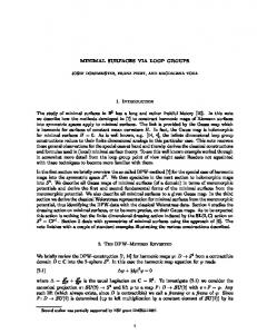
We assume multi-threaded programs are given in the form of an abstract state machine called thread transition diagram [16]. Such a diagram reflects the replicated nature of programs we consider: programs consisting of threads executing a given procedure defined over shared (“global”) and (procedure-)local variables. A thread transition diagram (TTD) is a tuple P = (S, L, R), where (6,0) (6,1) (6,2) (6,3) (6,4) – S is a finite set of shared states; (5,0) (5,1) (5,2) (5,3) (5,4) – L is a finite set of local states; – R ⊆ (S × L) × (S × L) is a(4,0)(finite) set of edges. (4,1) (4,2) (4,3) (4,4)

(6,3)

(6,4) (5,4)

(4,2)

(4,3)

(3,0) (3,1) (3,3) We (3,4) An element of V = S × L is S called thread(3,2)state. write (s → (s2 , l2 ) for 1 , l1 ) (3,2) (3,1) ((s1 , l1 ), (s2 , l2 )) ∈ R. We assume the TTD has a unique initial thread state, (2,0) (2,1) (2,2) (2,3) (2,4) denoted tI = (sI , lI ); the case(1,0)of multiple initial thread states is discussed in (1,1) (1,2) (1,3) (1,4) (1,0) (1,1) App. A. An example of a TTD is shown in Fig. 1(a). (0,0)

(0,1)

(0,2)

(0,3)

(0,4) (0,0) L

s

s (6,0)

(6,1)

(6,2)

(6,3)

(6,4)

(6,0)

(6,1)

(6,2)

(6,3)

(6,4)

(5,0)

(5,1)

(5,2)

(5,3)

(5,4)

(5,0)

(5,1)

(5,2)

(5,3)

(5,4)

(4,0)

(4,1)

(4,2)

(4,3)

(4,4)

(4,0)

(4,1)

(4,2)

(4,3)

(4,4)

(3,0)

(3,1)

(3,2)

(3,3)

(3,4)

(3,0)

(3,1)

(3,2)

(3,3)

(3,4)

(2,0)

(2,1)

(2,2)

(2,3)

(2,4)

(2,0)

(2,1)

(2,2)

(2,3)

(2,4)

(1,0)

(1,1)

(1,2)

(1,3)

(1,4)

(1,0)

(1,1)

(1,2)

(1,3)

(1,4)

(0,0)

(0,1)

(0,2)

(0,3)

(0,4)

(0,0)

(0,1)

(0,2)

(0,3)

(0,4)

(6,3) (6,3)

(6,4) (6,4) (5,4) (5,4)

(4,2) (4,2)

(4,3) (4,3)

(3,2) (3,2)

(1,1) l

l

(a)

(b)

(1,1)

(0,0)

(0,0)

(c)

Fig. 1. (a) A thread transition diagram P (initial state tI = (0, 0)); (b) the Expanded TTD P + with a path σ + ; (c) the SCC quotient graph P of P + , with quotient path σ. The black disc represents the loop in σ + (the other SCCs are trivial)

A TTD gives rise to a family, parameterized by n, of transition systems Pn = (Vn , Rn ) over the state space Vn = S × Ln , whose states we write in the form (s|l1 , . . . , ln ). This notation represents a global system state with shared component s, and n threads in local states li , for i ∈ {1, . . . , n}. The transitions of Pn , forming the set Rn , are written in the form (s|l1 , . . . , ln )  (s0 |l10 , . . . , ln0 ). This transition is defined exactly if there exists i ∈ {1, . . . , n} such that (s, li ) → (s0 , li0 ) and for all j 6= i, lj = lj0 . That is, our execution model is asynchronous: each transition affects the local state of at most one thread.1 The initial state set of Pn is {sI } × {lI }n . A path of Pn is a finite sequence of states in Vn whose first element is initial, and whose adjacent elements are 1

Dynamic thread creation is discussed at end of Sect. 6

4

Peizun Liu and Thomas Wahl

related by Rn . A thread state (s, l) ∈ S × L is reachable in Pn if there exists a path in Pn ending in a state with shared state s and some thread in local state l. A TTD also gives rise to an infinite-state transition system P∞ = (V∞ , R∞ ), whose set of states/transitions/initial states/paths is the union of the sets of states/transitions/initial states/paths of Pn , for all n ∈ N. We are tackling in this paper the thread state reachability problem: given a TTD P and a final thread state (sF , lF ), is (sF , lF ) reachable in P∞ ? It is easy to show that this question is decidable, by reducing P∞ to a well quasi-ordered system (WQOS) [1]: let the covers relation  over V∞ be defined as follows: (s|l1 , . . . , ln )  (s0 |l10 , . . . , ln0 0 ) whenever s = s0 and for all l ∈ L, |{i : li = l}| ≥ |{i : li0 = l}|. The latter inequality states that the number of threads in local state l “on the left” is at least the number of threads in local state l “on the right”. Relation  is a well quasi-order on V∞ , and (P∞ , ) satisfies the definition of a WQOS, in particular the monotonicity property required of  and . The proof of this property exploits the symmetry of the multi-threaded system: the threads execute the same program P: a state (s|l1 , . . . , ln ) can be compressed without loss of information into the counter notation (s|n1 , . . . , n|L| ), where nl = |{i : li = l}|. The thread state reachability question can now be cast as a coverability problem, which is decidable but of high complexity, e.g. EXPSPACE-hard for standard Petri nets [6], which are equivalent in expressiveness to infinite-state transition systems obtained from TTD [16]. A sound and complete algorithm to decide Algorithm 1 Bws(M, I, q) coverability for WQOS is the backward search Input: initial states I, algorithm by Abdulla et al. [2,1], a simple verfinal state q 6∈ I sion of which is shown on the right. Input is a 1: W := {q} ; U := {q} 2: while ∃w ∈ W WQOS M , a set of initial states I, and a non3: W := W \ {w} initial final state q. The algorithm maintains 4: for p ∈ CovPre(w) \ ↑ U a work set W of unprocessed states, and a set 5: if p ∈ I then U of minimal encountered states. It iteratively 6: “q coverable” computes minimal cover predecessors 0

0

CovPre(w) = min{p : ∃w  w : p  w } (1) starting from q, and terminates either by backward-reaching an initial state (thus proving coverability of q), or when no unprocessed vertex remains (thus proving uncoverability).

7: W := min(W ∪ {p}) 8: U := min(U ∪ {p}) 9: “q not coverable”

Alg. 1: infinite-state backward search. Symbol ↑ U stands for the upward closure of U : ↑ U = {u0 : ∃u ∈ U : u0  u}.

Strongly connected components. In this paper we also frequently make use of the following standard notions. Given a directed graph G, a strongly connected component (SCC) is a maximal set C of vertices such that for any two vertices c1 and c2 in C, there is a path in C from c1 to c2 . If the subgraph of G induced by C has no edge, C is called trivial.

Concolic Unbounded-Thread Reachability via Loop Summaries

5

The SCC quotient graph G of G has exactly one vertex for each SCC of G, and no other vertices; we identify each vertex of G with the SCC it represents. An edge (C1 , C2 ) exists in G whenever C1 6= C2 and there is a G-edge from some vertex in C1 to some vertex in C2 . For a vertex v, we denote by v the unique SCC that v belongs to (hence, by identification, v is also a vertex in G). Since each cycle of G is contained entirely in one SCC, and nodes in G have no self-loops, G is acyclic.

3

Pathwise Unbounded-Thread Reachability: Overview

Our approach for accelerating backward reachability analysis is two-phased. The first phase constructs from P an abstract structure P, with the property that any thread state reachable in P∞ (i.e., for any number of threads) is also reachable in P when executed by a single thread. Structure P thus overapproximates the thread-state reachability problem for P to a much simpler sequential reachability problem. Technically, the abstraction first adds certain edges to P, and then collapses strongly connected components to obtain P, which is hence acyclic. Note that this first phase performs no exploration and is in fact independent of the underlying reachability algorithm being accelerated. In the second phase, we analyze each path σ in the acyclic structure P from tI to tF separately, if any. We now distinguish: if σ visits only simple SCCs, by which we mean SCCs that represent simple loops, then we call σ simple, and we precisely summarize the effect of traversing the path using Presburger formulas.2 Instead of executing Alg. 1, we solve these Presburger constraints, in effect accelerating the algorithm, losslessly, along loop-free path segments and simple loops. If σ visits at least one spaghetti SCC — an SCC that represents more than a simple loop (e.g. a loop nest) — then we call σ spaghetti as well and explore it using Alg. 1, restricted to the edges along σ. At the end of this section we illustrate the overall process in more detail. We first introduce the acyclic quotient structure P. A Single-Threaded Abstraction of P∞ . A key operation employed during backward search is what we call expansion of a global state: the addition of a thread in a suitable local state during the computation of the cover preimage (1). We can simulate the effect of such expansions without adding threads, by allowing a thread to change its local state in certain disciplined ways. To this end, we expand the TTD data structure as follows. Def. 1 Given a TTD P = (S, L, R), an expansion edge is an edge of the form ((s, l), (s, l0 )) (same shared state) such that l 6= l0 and the following holds: – there exists an edge of the form . . . → (s, l) in R, and – there exists an edge of the form (s, l0 ) → . . . in R, or (s, l0 ) = (sF , lF ). 2

Simple SCC nodes (representing a simple loop) are not to be confused with trivial SCC nodes (representing a single node). Simple nodes are by definition non-trivial

6

Peizun Liu and Thomas Wahl

The Expanded TTD (ETTD) of P is the structure P + = (S, L, R+ ) with R+ = R ∪ {e : e is an expansion edge}. To distinguish the edge types in P + , we speak of real edges (in R) and expansion edges. Intuitively, expansion edges close the gap between two real edges whose target and source, respectively, differ only in the local state. This can be seen in Fig. 1(b), which shows the ETTD generated from the TTD in Fig. 1(a). In the graphical representation, expansion edges run horizontally and are shown as dashed arrows (s, l) 99K (s, l0 ). To facilitate the identification and treatment of loops, we collapse the ETTD P + into its (acyclic) SCC quotient graph, denoted P. An example is shown in Fig. 1(c). For ease of presentation, we assume that both the initial and final thread states tI and tF of P form single-node SCCs in P, i.e. loops occur only in the interior of a path. This can be enforced easily using artificial states. Being acyclic, the quotient graph P contains only finitely many paths between any two nodes. It also has another key property that makes it attractive for our approach. Let us interpret P as a sequential transition system. That is, when we speak of reachability of a thread state and paths in P, we assume P is executed by a single thread from tI . (In contrast, the semantics of P is defined via the unbounded-thread transition system P∞ .) Given these stipulations, P overapproximates P, in the following sense: Lem. 2 If thread state tF is reachable in P∞ , then tF is also reachable in P. By Lem. 2, if tF is not reachable from tI in P (a simple sequential reachability problem), it is not reachable in P∞ . In that case our algorithm immediately returns “unreachable” and terminates. If tF is reachable in P, we cannot conclude reachability in P∞ , as can be seen from Fig. 1: thread state tF := (6, 4) is easily seen to be unreachable in P∞ , no matter how many threads execute the diagram P in (a). But tF is obviously sequentially reachable in P (c). In the rest of this paper we describe how to decide, for each path σ in P from tI to tF , whether it actually witnesses reachability of tF in P∞ . To give an overview of this process, consider a quotient path σ with one simple SCC node. One such path is schematically depicted in Fig. 2, where we have zoomed in on the SCC node `i in order to show the simple loop of P + collapsed inside it. To analyze reachability of tF in P∞ , we first consider the path segment from tF to the exit point of the loop (see Fig. 2). The exit point is the unique node of P + abstracted by SCC node `i that is first encountered when the quotient path σ is explored backward. Our approach builds a symbolic summary for this path segment. We then do the same for the simple loop collapsed inside `i , and for the path from the entry point of the loop back to tI . These summaries are combined conjunctively into a single Presburger expression ϕ over a parameter κ that represents the number of iterations through the loop represented by `i . We now conjoin ϕ with the constraint that, when backward-reaching tI along σ, no thread resides in any local state other than lI . This condition ensures that the global state constructed

Concolic Unbounded-Thread Reachability via Loop Summaries exit point `m−1

tF

hi hm

hm−1 `m

entry point `1

`i

h0

hi−1 `i+1

7

`i−1

tI

Fig. 2. A path σ in the acyclic structure P with a non-trivial and magnified SCC node `i , representing some kind of loop structure in P +

via symbolic backward execution is of the form {sI } × {lI }n , i.e. it is initial. The claim that tF is reachable in P∞ is then equivalent to the satisfiability of the overall formula; a satisfying assignment to κ specifies how many times the loop in `i needs to be traversed. In Sect. 4 and 5 we describe how loop-free path segments and simple loops, respectively, are summarized, to obtain a symbolic characterization.

4

Presburger Summaries for Loop-Free Path Segments

Consider a path segment σ in P with only trivial (singleton) SCC nodes in its interior; we call such segments loop-free. (The start and end state of σ may still be non-trivial SCC nodes; the loops contracted by these SCC nodes are not considered in this section.) The real and expansion edges along σ suggest a firing sequence of edges during an exploration of P∞ using Alg. 1. Each real edge corresponds to a thread state change for a single thread; each expansion edge corresponds to the expansion of the current global state. More precisely, given a global state of the form (s0 |l10 , . . . , ln0 ), Alg. 1 computes cover preimages (Eq. (1)), by first firing edges of R backward whose targets equal one of the thread states (s0 , li0 ). Second, for each edge e whose target (s0 , l0 ) (with shared state s0 ) does not match any of the thread states (s0 , li0 ), Alg. 1 expands the global state, by adding one thread in local state l0 , followed by firing e backward, using the added thread.3 The steps performed by Alg. 1 can be expressed in terms of updates to localstate counters. Let edge e be of the form (s, l) → (s0 , l0 ). If the current global state (s0 |l10 , . . . , ln0 ) contains a thread in local state l0 , firing e backward amounts to decrementing the counter nl0 for the target l0 , and incrementing the counter nl for the source l. If the current global state does not contain a thread in local state l0 , we first expand the state by adding such a thread, followed by firing e backward. Together the step amounts exactly to an increment of nl . We can execute these steps symbolically, instead of concretely, by traversing path segment σ backward and encoding the corresponding counter updates 3

We exploit the fact that cover preimages in systems induced by TTDs increase the number of threads in a state by at most 1 (see [20, Lemma 1] for a proof)

8

Peizun Liu and Thomas Wahl

Algorithm 2 Summary of a loop-free path segment Input: path σ = t1 , . . . , tk in P, i.e. (ti , ti+1 ) ∈ R+ for 1 ≤ i < k ; local state l 1: ei := (ti , ti+1 ) for 1 ≤ i < k , (si , li ) := ti for 1 ≤ i ≤ k 2: summary := "nl " B summary is a string 3: for i := k − 1 downto 1 4: if ei ∈ R and li = l then 5: summary := summary."+1" B . = string concatenation 6: if ei ∈ R and li+1 = l then 7: summary := summary."-1" 8: if ei ∈ R+ \ R and li = l then 9: summary := summary."1+1" 10: return summary

described in the previous paragraph as logical constraints over the local-state counters. The constraints are expressible in Presburger (linear integer) arithmetic. To demonstrate this, we introduce some light notation. For x, y ∈ Z and b ∈ N, let xb y = max{x+y, b}. Intuitively, xb y is “x+y but at least b”. When b = 0, we omit the subscript. We also use x b y as a shorthand for x b (−y) (= max{x − y, b}). For example, x  1 equals x − 1 if x ≥ 1, and 0 otherwise. Neither b nor b are associative: (1  2)  −3 = 0 6= 1 = 1  (2  −3). We therefore stipulate: these operators associate from left to right, and they have the same binding power as + and − . Operators / in Presburger formulas are syntactic sugar: we can rewrite a formula Γ containing x b y, using a fresh variable v per occurrence: Γ

≡ (Γ |(xb y)→v ) ∧ ((x + y ≥ b ∧ v = x + y) ∨ (x + y < b ∧ v = b))

(2)

where α|β→γ denotes substitution of γ for β in α. The summary of loop-free path segment σ is computed separately for each local state l: Alg. 2 symbolically executes σ backward; for certain edges a “contribution” to counter nl is recorded, namely for each edge of R+ that is adjacent to local state l, but only if it is real, or it is an expansion edge that starts in local state l. Note that the three if clauses in Alg. 2 are not disjoint: the first two both apply when edge ei is “vertical”: it both enters and exits local state l. In this case the two contributions cancel out. The summary of path σ for local state l defines a function Σl : N → N that summarizes the effect of path σ on counter nl . The summary functions for the short path in Fig. 3 are shown next to the figure. These examples illustrate how we can encode a loop-free quotient path into a quantifier-free Presburger formula. The formula for Σ0 (n0 ) implies that if we traverse the path backward from a state with n0 = 0 threads in local state 0, at the end there will be Σ0 (0) = 0  1 + 1 = 1 thread in local state 0. If we start with n0 = 1, we also end up with n0 = 1. Note that the path cannot be traversed backward starting with n2 = 0, since its endpoint is thread state (2, 2). Non-trivial SCC nodes along σ are contractions of loops in the expanded structure P + , to the effect that paths in P + are no longer finite; their summaries

Concolic Unbounded-Thread Reachability via Loop Summaries s

9

Summary functions for local states l = 0, 1, 2: (2,0)

(2,1)

(2,2)

(1,0)

(1,1)

(1,2)

(0,0)

(0,1)

(0,2)

Σ0 (n0 ) = n0  1 + 1 − 1 + 1 = n0  1 + 1 Σ1 (n1 ) = n1 + 1 Σ2 (n2 ) = n2 − 1 Examples: Σ0 (0) = 1, Σ0 (1) = 1, Σ1 (0) = 1, Σ2 (1) = 0 .

l

Fig. 3. A loop-free quotient structure P with a vertical real edge

cannot be obtained by symbolic execution. Instead we will determine a precise summary of simple loops that is parameterized by the number κ of times the loop is executed. Spaghetti loops are discussed in Sect. 6.

5

Presburger Summaries for Simple Loops

In this section we generalize path summaries to the case of simple SCCs, formed by a single simple loop, i.e., a single cyclic path without repeated inner nodes. We aim at an exact solution in the form of a closed expression for the value of local state counter nl after Alg. 1 traverses the loop some number of times κ. In this section, since we need to “zoom in” to SCCs collapsed into single nodes in P, we instead look at paths in P + . Recall that for a loop-free path σ + , the value of counter nl after Alg. 1 traverses σ + can be computed using σ + ’s path summary function Σl , determined via symbolic execution (Alg. 2). In the case that σ + is a loop, we would like to obtain a summary formula parameterized by the number κ of times the loop is executed (we cannot replicate σ + ’s summary function κ times, since κ is a variable). To this end, let σ + = t1 , . . . , tk with tk = t1 be a loop in P + , and define (si , li ) := ti for 1 ≤ i ≤ k. Let δl = |{i : 1 ≤ i < k : (ti , ti+1 ) ∈ R ∧ li = l}| − |{i : 1 ≤ i < k : (ti , ti+1 ) ∈ R ∧ li+1 = l}|

(3)

be the real-edge summary δl ∈ Z of σ + , i.e. the number of real edges along σ + that start in local state l, minus the number of real edges along σ + that end in l. Value δl summarizes the total contribution by real edges to counter nl as path σ + is traversed backward: real edges starting in l increment the counter, those ending in l decrement it. Let further bl = Σl (1) if σ + ends in local state l (in this case the backward traversal must start with at least 1 thread in l), and bl = Σl (0) otherwise. Thm. 3 Let superscript

(κ)

denote κ function applications. Then, for κ ≥ 1,

Σl (κ) (nl ) = nl bl δl bl (κ − 1) · δl .

(4)

10

Peizun Liu and Thomas Wahl

Recall that  is not associative (it associates from left to right); the right-hand side of Eq. (4) can generally not be simplified to nl bl κ · δl . Intuitively, the term nl bl δl marks the contribution to counter nl of the first loop traversal, while (κ − 1) · δl marks the contribution of the remaining κ − 1 traversals. Example. We show how the unreachability of thread state (6, 4) for the TTD in Fig. 1 is established. For each local state l ∈ {0, . . . , 4}, the following constraints are obtained (after simplifications) from summaries of the loop-free path segment from (6, 4) to (3, 1) (“loop exit point”), the loop inside the SCC node (black disc) using Thm. 3, and the loop-free path segment from (1, 0) (“loop entry point”) via (1, 1) to the initial thread state (0, 0). Parameter κ is the number of times the loop is executed: n0 n1 n2 n3 n4

: : : : :

0 0 0 2 2 2 (κ − 1) · 2 3 3 0 1 0 1 −1 1 (κ − 1) · −1 0 −3 0 2 2 0 −1 0 (κ − 1) · −1 0 0 0 0 −2 0 0 0 (κ − 1) · 0 0 0 1 1 0 0 0 0 (κ − 1) · 0 0 0

≥ = = = =

1 0 0 0 0

The equation for n4 simplifies to 1 = 0 and thus immediately yields unsatisfiability. Since there is only one path in P, we conclude unreachability of tF = (6, 4). In contrast, for target thread state (6, 3), the equations for n3 and n4 both reduce to true. The conjunction of all five equations reduces to 1 0 (κ − 1) · (−1) = 0. This formula is satisfied by κ = 2, witnessing reachability of (6, 3) via a path containing two full iterations of the loop inside the SCC.

6

Pathwise Unbounded-Thread Reachability

Consider an SCC along quotient path σ that represents several distinct simple loops in P + . An example is an SCC with two loops A and B that have one point in common and form an “eight” ∞. Such a double loop features paths of the form (A|B)∗ , where in each iteration there is a choice between A and B. Our loop acceleration technique from Sect. 5 does not apply to such paths. To solve this problem, we exploit the synergy between the pathwise analysis suggested by the acyclic structure P, and the fact that certain — namely, simple — paths can be processed using the technique described in Sect. 4 and 5. Spaghetti paths are explored by Alg. 1, but restricted to the narrow “slice” of P marked by the quotient path in P. This algorithm is shown in Alg. 3. It takes as input the TTD P, as well as the initial and final thread states, tI and tF . The algorithm begins by building the quotient structure P. This acyclic structure is now analyzed pathwise. For each path σ from tI to tF in P, we first decide whether it is spaghetti or simple. • If σ is spaghetti (visits some spaghetti SCCs), we explore it using Alg. 1 (Line 4). More precisely, let P σ be the restriction of the given TTD to the

Concolic Unbounded-Thread Reachability via Loop Summaries

11

Algorithm 3 Pathwise Reachability Input: TTD P, thread states tI , tF 1: P + := expanded TTD, P := SCC quotient graph of P + 2: for each path σ in P from tI to tF 3: if σ is spaghetti then 4: if Bws((P σ )∞ , ∪n∈N {sI } × {lI }n , tF ) = “tF coverable” then 5: return “tF reachable in P∞ from tI ” 6: else 7: m := number of non-trivial SCCs visited by σ B these SCCs are all simple 8: φ(κ1 , . . . , κm ) := Presburger summary for σ B Sect. 4, 5 9: if φ(κ1 , . . . , κm ) satisfiable then 10: return “tF reachable in P∞ from tI ” 11: return “tF unreachable in P∞ from tI ”

edges along σ, including any edges collapsed inside SCCs. Let further (P σ )∞ be the infinite-state transition system derived from P σ as described in Sect. 2. We pass this transition system to procedure Bws (Alg. 1), along with the unchanged set of initial states, and the unchanged final state (which is also the end-point of σ). If this invocation results in “coverable”, tF is reachable in P∞ from tI , which is hence returned in Line 5. • If σ is simple (does not visit any spaghetti SCCs), we can accelerate exploration along it using the techniques introduced in Sect. 4 and 5. We build a Presburger summary for the path, parameterized by the loop iteration counts κi , one for each loop.4 If this formula is satisfiable, again we have that tF is reachable in P∞ from tI . The assignment to the κi gives the number of times each loop needs to be traversed; from this data a multi-threaded path through P can easily be constructed. If none of the paths σ results in the answer “coverable” by either concrete or symbolic exploration, tF is unreachable in P∞ from tI , which is hence returned as the answer. Note that this happens in particular if there is no path at all from tI to tF in P. Correctness. Alg. 3 terminates since P is acyclic, so the loop in Line 2 goes through finitely many iterations. Partial correctness follows from the following two claims. Let σ be a quotient path considered in Line 2. 1. If σ is spaghetti, then Alg. 3 outputs “reachable” in Line 5 iff tF is reachable in P∞ along the edges represented by σ. 2. If σ is simple, then Alg. 3 outputs “reachable” in Line 10 iff tF is reachable in P∞ along the edges represented by σ. Claim 1 is proved using soundness and completeness of Alg. 1. Claim 2 is proved using Thm. 3. Given these claims, we obtain: 4

Loop-free paths (m = 0) can be processed either using Alg. 1, or via summaries.

12

Peizun Liu and Thomas Wahl

Cor. 4 (Soundness) If Alg. 3 returns “reachable” (Line 5 or 10) or “unreachable” (Line 11), then tF is reachable or unreachable, respectively, in P∞ . Proof. • If Alg. 3 returns “reachable”, then it does so for some σ, in Lines 5 or 10. The fact that tF is actually reachable in P∞ follows from one of the two claims above, depending on whether σ is spaghetti or simple. • If Alg. 3 returns “unreachable”, then it does not reach Lines 5 or 10, for any σ. By the above two claims, tF is not reachable in P∞ along the edges represented by any quotient path. The fact that then σ is not reachable in P∞ at all follows from the proof of Lem. 2: the proof shows that, if tF is reachable, then there exists a quotient path in P from tI to tF such that tF is reachable in P∞ along the edges represented by that quotient path. 2

Implementation. Our technique is implemented in a reachability checker named Cutr5 . We discuss some details on the implementation of Alg. 3 in Cutr. Line 2 selects potential paths in P. Since we can abort the algorithm once a path is found that witnesses reachability, it makes sense to rank the paths by “promise” of ease of processing: we begin with loop-free paths, i.e. those with only trivial SCCs, followed by paths with simple SCCs whose edges are all real, followed by paths with simple SCCs that feature expansion edges. Finally we select paths with spaghetti loops inside SCCs. The length of a path is secondary. In order to call Bws in Line 4 on the TTD restricted to the edges represented by σ, there is no need to construct P σ a priori. Instead, when computing cover preimages, we make sure to only fire TTD edges belong σ and its loops. To keep our computational model simple, we have excluded from the formalization in Sect. 2 dynamic thread creation, where threads are spawned during the execution of the program. This feature does not formally add expressive power, but is often included for its presence in multi-threaded software. Our implementation does support thread creation. Symbolically backward-executing a thread creation edge is straightforward: the counter of the local state of the spawned thread must be decreased, since that thread does not exist in the source state. Our implementation performs some book-keeping to ensure the backwardexecutability of such an edge: both the local state of the spawned thread, as well as that of the spawning thread must exist in the successor state, since the spawning thread does not change its state (it only side-effects the thread creation).

7

Empirical Evaluation

In this section we provide experimental results obtained using Cutr. The goal of the experiments is to measure the performance impact of the presented approach compared to the backward search Alg. 1. We expect our approach to improve the latter, as it is short-cutting standard backward exploration across simple loops and linear path segments. The question is whether solving Presburger equations instead of concretely exploring loops actually amounts to speed-up. 5

Cutr “=” Concolic Unbounded-Thread Reachability analysis.

Concolic Unbounded-Thread Reachability via Loop Summaries

13

Experimental Setup. We collected an extensive set of benchmarks, 173 in total, which is organized into two suites. The first suite contains 124 TTDs obtained from Boolean programs (BPs), which are in turn obtained from C source programs (taken from [16]) via predicate abstraction. As TTDs are equivalent in expressiveness to certain forms of Petri nets [8,16], we include PN examples in our benchmark collection. The second suite therefore contains 49 BP min. max. 5 257 TTDs obtained from PNs (taken from [8]). While PNs are not |S| |L| 14 4097 the main focus of this work, we were hoping to get insights |R| 18 20608 into how complex concurrency affects our approach, as the PN min. max. PNs available to us exhibited more challenging concurrent |S| 6 18234 behaviors than the BPs. The table on the right shows size |L| 6 332 ranges of the benchmarks. |R| 13 27724 We use Z3 (v4.3.2) [21] as the Presburger solver. For each benchmark, we consider verification of a safety property. In the case of BP examples, the property is specified via an assertion. There are 87 safe instances in total: 56 of the BPs, and 31 of the PNs. All experiments are performed on a 2.3GHz Intel Xeon machine with 64 GB memory, running 64-bit Linux. Execution time is limited to 30min, and memory to 4 GB. All benchmarks and our tool are available online6 . Comparison. We first consider TTDs obtained from BPs, the target of this work. The runtime comparison results are given in the top left part of Fig. 4. The results demonstrate that Cutr performs much better than Bws. In some cases, runs that time out in Bws can be successfully solved by Cutr within 30min; in contrast, there is only one example such that Bws successfully completes while Cutr runs time out. The latter situation can be explained by the path explosion: there are more than 5000 paths for this example. We now consider TTDs obtained from PNs; see top right of Fig. 4. Here we see little performance difference. Investigating this further, we found that for Petri nets the density of TTD edges is higher (explained by their more complex structure and the relatively less organization and control in the concurrent systems represented by Petri nets, compared to programs). This has two consequences: (i) there are few but large SCCs, and (ii) most of them are spaghetti. As a result, there are few paths through the quotient structure, and almost all of them are explored via calling Bws. This makes the whole process essentially equivalent to a single call to Bws. The curves at the bottom left of Fig. 4 illustrate that Bws utilizes less memory on small BP benchmarks, an effect can be explained by the overhead of pathwise analysis and Z3. On large examples Cutr tends to need less memory resource than Bws. The memory comparison for PNs shows similar results. The performance impact of our acceleration approach, on both runtime and memory, can be summarized as follows. Our method analyzes a specific path at a time. If tF is reachable, there is a good chance Cutr can find a solution early, due to the ranking of paths, some of which permit quick decisions. Although 6

Webpage: http://www.ccs.neu.edu/home/lpzun/cutr

Peizun Liu and Thomas Wahl RO

103

RO unsafe BP safe BP

103 102 Cutr (sec.)

Cutr (sec.)

102

unsafe PN safe PN

101 100

101 100

101

102

103

100

RO

100

Bws (sec.)

103

RO Bws Cutr

3

10 Memory Usage (MB.)

Memory Usage (MB.)

10

102

Bws (sec.)

RO

3

101

RO

14

102

101

20

40

60

80

BP Benchmark

100

124

Bws Cutr

102

101

10

20

30

40

49

PN Benchmark

Fig. 4. Performance impact (BP/PN = TTD from BP/PN). RO stands for “out of resources”: the run reached the time or the memory limit before producing a result. • Top row shows the comparisons of execution time. Left: comparison on BPs; Right: comparison on PNs. Each plot represents execution time on one example. • Bottom row shows the comparison of memory usage. Left: comparison on BPs; Right: comparison on PNs. The curves are sorted by the memory usage of Cutr.

Cutr relies on backward search to cross nested loops, the cost of that is limited as such exploration is confined to a small fragment of the TTD. In the extreme, the entire TTD contains only one path with spaghetti loops. In this case Cutr falls back on backward search.

8

Related Work

Groundbreaking results in infinite-state system analysis include the decidability of coverability in vector addition systems (VAS) [17], and the work by German and Sistla on modeling communicating finite-state threads as VAS [13]. Numerous results have since improved on the original procedure in [17] in practice

Concolic Unbounded-Thread Reachability via Loop Summaries

15

[11,12,22,23]. Others extend it to more general computational models, including well-structured [10] or well quasi-ordered transition systems [2,1]. Recent theoretical work by Leroux employs Presburger arithmetic to solve the VAS global configuration reachability (not coverability) problem. In [18], it is shown that a state is unreachable in the VAS iff there exists an “inductive” Presburger formula that separates the initial and final states. The theoretical complexity of this technique is mostly left open. Practicality is not discussed and doubted later by the author in [19], where a more direct approach is presented that permits the computation of a Presburger definition of the reachability set of the VAS in some cases, e.g. for flatable VAS. Reachability can then be cast as a Presburger decision problem. The question under what exact conditions the VAS reachability set is Presburger-definable appears to be undecided. The results referenced above are mainly foundational in nature and target generally harder (even undecidable) reachability questions than we do in this paper. We emphasize that our motivation for acceleration is not to ensure convergence of (otherwise possible diverging) fixpoint computations. Instead, our goal here was to show, for the decidable problem of TTS thread state reachability, (i) how to practically compute a Presburger encoding whose satisfiability implies reachability of the thread state, and (ii) that the resulting (quantifierfree) formulas are often easy to decide, thus giving rise to an efficient algorithm. Existing (typically forward) acceleration techniques for infinite-state systems [9,5,15] were inspirational for this paper. In recent work, Petri net marking equations are used to reduce the coverability problem to linear constraint solving [8]. Follow-up work investigates a similar approach for thread-transition systems [3]. Like the present work, these approaches benefit from advances in SMT technology and in fact have proved to be efficient. On the other hand, they are incomplete (the constraints overapproximate coverability). Our goal here was to retain (soundness and) completeness, and to investigate at what cost this can be achieved.

9

Conclusion

In this paper, we have presented an approach for accelerating a widely-applicable infinite-state search algorithm for systems of unbounded numbers of threads. A key ingredient is the construction of an acyclic quotient of the input program, which in turn enables a finite path-by-path analysis. Loop-free paths and paths with only simple loops can be collapsed without approximation into Presburger arithmetic constraints that symbolically summarize the effect of executing the backward search algorithm along these paths in the multi-threaded program. Each path passing through loop nests is processed via standard explicit-state backward search but confined to this particular path. We have demonstrated the power of this method for proving and refuting safety properties of an extensive set of TTDs obtained from Boolean program benchmarks. We conclude that partial but exact symbolic acceleration of existing sound and complete infinitestate search algorithms is very much feasible, and in fact very beneficial.

16

Peizun Liu and Thomas Wahl

References 1. Abdulla, P.A.: Well (and better) quasi-ordered transition systems. Bulletin of Symbolic Logic 16(4), 457–515 (2010) 2. Abdulla, P.A., Cerans, K., Jonsson, B., Tsay, Y.K.: General decidability theorems for infinite-state systems. In: LICS. pp. 313–321 (1996) 3. Athanasiou, K., Liu, P., Wahl, T.: Unbounded-thread program verification using thread-state equations. In: IJCAR. pp. 516–531 (2016) 4. Ball, T., Majumdar, R., Millstein, T., Rajamani, S.K.: Automatic predicate abstraction of c programs. In: PLDI. pp. 203–213 (2001) 5. Bardin, S., Finkel, A., Leroux, J., Schnoebelen, P.: Flat acceleration in symbolic model checking. In: ATVA. pp. 474–488 (2005) 6. Cardoza, E., Lipton, R.J., Meyer, A.R.: Exponential space complete problems for Petri nets and commutative semigroups: Preliminary report. In: STOC. pp. 50–54 (1976) 7. Donaldson, A., Kaiser, A., Kroening, D., Wahl, T.: Symmetry-aware predicate abstraction for shared-variable concurrent programs. In: CAV. pp. 356–371 (2011) 8. Esparza, J., Ledesma-Garza, R., Majumdar, R., Meyer, P., Niksic, F.: An SMTbased approach to coverability analysis. In: CAV. pp. 603–619 (2014) 9. Finkel, A., Leroux, J.: How to compose Presburger-accelerations: applications to broadcast protocols. In: FSTTCS. pp. 145–156 (2002) 10. Finkel, A., Schnoebelen, P.: Well-structured transition systems everywhere! Theor. Comput. Sci. 256(1-2), 63–92 (2001) 11. Geeraerts, G., Raskin, J.F., Begin, L.V.: Expand, enlarge and check: New algorithms for the coverability problem of WSTS. J. Comput. Syst. Sci. 72(1), 180–203 (2006) 12. Geeraerts, G., Raskin, J.F., Begin, L.V.: On the efficient computation of the minimal coverability set for Petri nets. In: ATVA. pp. 98–113 (2007) 13. German, S.M., Sistla, A.P.: Reasoning about systems with many processes. J. ACM 39(3), 675–735 (Jul 1992) 14. Graf, S., Sa¨ıdi, H.: Construction of abstract state graphs with PVS. In: CAV. pp. 72–83 (1997) 15. Jonsson, B., Saksena, M.: Systematic acceleration in regular model checking. In: CAV. pp. 131–144 (2007) 16. Kaiser, A., Kroening, D., Wahl, T.: A widening approach to multithreaded program verification. ACM Trans. Program. Lang. Syst. 36(4), 14 (2014) 17. Karp, R.M., Miller, R.E.: Parallel program schemata. Journal of Computer and System Sciences 3(2), 147–195 (1969) 18. Leroux, J.: The general vector addition system reachability problem by Presburger inductive invariants. In: LICS. pp. 4–13 (2009) 19. Leroux, J.: Presburger vector addition systems. In: LICS. pp. 23–32 (2013) 20. Liu, P., Wahl, T.: Infinite-state backward exploration of Boolean broadcast programs. In: FMCAD. pp. 155–162 (2014) 21. de Moura, L., Bjørner, N.: Z3: An efficient SMT solver. In: TACAS. pp. 337–340 (2008) 22. Reynier, P.A., Servais, F.: Minimal coverability set for Petri nets: Karp and Miller algorithm with pruning. In: Petri Nets. pp. 69–88 (2011) 23. Valmari, A., Hansen, H.: Old and new algorithms for minimal coverability sets. In: Petri Nets. pp. 208–227 (2012)

Concolic Unbounded-Thread Reachability via Loop Summaries

17

Appendix A

Uniqueness of the Initial State

In our problem formulation we have assumed a unique initial state of the program (TTD) executed by each thread. This essentially fixes the start state of each TTD path we have to process. The more general case of multiple initial states can of course be handled by considering each initial state in turn. However, in many practical cases, the general case can be reduced to the unique-initial-thread-state case without affecting thread state reachability. Suppose the initial thread state set T of the given TTD P satisfies the following “box” property: ∀(s, t) ∈ T, (s0 , t0 ) ∈ T : (s, t0 ) ∈ T, (s0 , t) ∈ T .

(5)

This holds if T is (already) a singleton. More generally, it holds if all states in T have the same shared state,7 and it holds if all states in T have the same local state. It also holds of a set T whose elements form a complete rectangle in the graphical representation of P. To enforce a unique initial thread state, we build a new TTD P 0 that is identical to P, except that it has a single initial thread state tI = (sI , lI ) with fresh shared and local states sI , lI , and the following additional edges: (sI , lI ) → (s, l)

such that (s, l) ∈ T ,

(s, lI ) → (s, l)

such that (s, l) ∈ T .

and

(6) (7)

We see that the cost of obtaining P 0 from P is linear in the size of the initial state set T . Suppose now some thread state t0 = (s0 , l0 ) is reachable in Pn , for some n. Then there exists a path from some global state (sJ |l1 , . . . , ln ) such that (sJ , li ) ∈ T for all i, to a global state with shared component s0 and some thread in local state l0 . We can attach, to the front of this path, the prefix (sI |lI , . . . , lI )



(sJ |l1 , lI , lI , . . . , lI )



(sJ |l1 , l2 , lI , . . . , lI )



(sJ |l1 , l2 , l3 , . . . , ln ) ,

···

with the underlined symbols changed. The new path reaches t0 in Pn0 . Conversely, suppose some thread state t0 = (s0 , l0 ) such that s0 6= sI , l0 6= lI is reachable in Pn0 , for some n. Then there exists a path p0 from {sI } × {lI }n to a global state with shared component s0 and some thread in local state l0 . The very first transition of p0 is by some thread executing an edge of type (6), 7

Shared states are formed by valuations of shared (global) Boolean variables, which in turn store values of predicates over C program variables. If these C program variables are themselves global, they are initialized by the operating system and hence unique.

18

Peizun Liu and Thomas Wahl

since those are the only edges leaving the unique initial state (sI , lI ). Let that be thread number i, and let (s, l) ∈ T be the new state of thread i. Consider now an arbitrary thread j ∈ {1, . . . , n} \ {i}; its local state after the first transition along p0 is lI . • If thread j is never executed along p0 , we build a new path p00 by inserting edge (s, lI ) → (s, l), executed by thread j, right after the first transition in p0 . This is a valid edge (of type (7)) since (s, l) ∈ T . The edge moves thread j into an initial thread state (s, l) ∈ T . The modified state sequence remains a valid path in Pn0 since no shared states have been changed, and thread j is inactive henceforth. • If thread j is executed along p0 , then the first edge it executes must be of type (7), since again this is the only way to get out of local state lI . Let (¯ s, ¯l) ∈ T be the state of thread j after executing this first edge. Then (s, lI ) → (s, ¯l) is a valid edge (of type (7)): from (s, l) ∈ T and (¯ s, ¯l) ∈ T , we conclude (s, ¯l) ∈ T , 00 by property (5). We now build a new path p , by removing from p0 thread j’s first transition, and instead inserting, right behind the first transition of p0 , a transition where thread j executes edge (s, lI ) → (s, ¯l): i

p0 :: (sI , lI ) → (s, t) ,

...

j

, (¯ s, lI ) → (¯ s, ¯l)

becomes j i p00 :: (sI , lI ) → (s, t) , (s, lI ) → (s, ¯l) ,

...

(here we add a thread index on top of an edge’s arrow, to indicate the identity of the executing thread). The modified state sequence remains a valid path in Pn0 , since the shared states “match” and are not changed by any of the removed or inserted edges. Moving the local state change of thread j (from lI to ¯l) forward leaves the path intact, since the original edge (¯ s, lI ) → (¯ s, ¯l) was thread j’s first activity. This procedure is applied to every thread j 6= i, with the result that, after the first n transitions, all threads are in a state belonging to T . The suffix of p00 following these transitions reaches t0 in Pn . 2

B

Proof of Lemma 2

Lem. 2 If thread state tF is reachable in P∞ , then tF is also reachable in P. Proof : We show that tF is reachable in P + ; the fact that tF is reachable in P then follows from standard properties of the SCC quotient graph. Let tF = (sF , lF ), and tI = (sI , lI ) be the initial state. Since tF is reachable in P∞ = ∪∞ n=1 Pn , let n be such that tF is reachable in Pn via a witness path p: p :: (sI | lI , . . . , lI ) | {z } n



···



(sF |l1 , . . . , li−1 , lF , li+1 , . . . , ln ).

(8)

Concolic Unbounded-Thread Reachability via Loop Summaries

19

Let further (ei ) := (e1 , . . . , ez ) be the sequence of TTD edges executed along p. We drop all “horizontal” edges from (ei ), i.e. edges of the form (s, ·) → (s, ·), to obtain a subsequence (gi ) := (g1 , . . . , gz0 ) (z 0 ≤ z). Given (gi ), we construct a path σ from tI to tF in P + , by processing the edges gi , defined recursively as follows: (1) Edge g1 is processed by copying it to σ. (2) Suppose edge gk−1 has been processed, and suppose its target state is (s, li ). Edge gk ’s source state has shared component s as well, since edges gk−1 and gk are consecutive in p, except for some horizontal edges in between that may have been dropped, but these do not change the shared state. So let gk ’s source state be (s, lj ). Edge gk is now processed as follows. If li = lj , append gk to σ. Otherwise, first append (s, li ) 99K (s, lj ) to σ, then gk . Note that (s, li ) 99K (s, lj ) is a valid expansion edge in R+ , since there exist two non-horizontal edges, gk−1 and gk , adjacent to the expansion edge’s source and target, respectively. Step (2) is repeated until all edges gi have been processed. It is clear by construction that σ is a valid path in P + , and that it starts in tI = (sI , lI ). We finally have to show that it ends in tF = (sF , lF ). It may in fact not: let (sF , lf ) be the target state of the final edge gz0 ; lf may or may not be equal to lF . If it is not, we append an edge (sF , lf ) 99K (sF , lF ) to σ. This is a valid expansion edge by Def. 1, and σ now ends in tF , which is hence reachable in P + . 2

C

Proof of Theorem 3

Before we turn to this proof, we establish a lemma that uses the δl ’s defined in Sect. 5 to compactly determine local state l’s summary along σ + . Lem. 3 Let bl = Σl (1) if lk = l (path σ + ends in local state l), and bl = Σl (0) otherwise. Then Σl (nl ) = nl bl δl .

The lemma suggests: in order to determine local state l’s summary function in compact form, first compute the constant Σl (1) (or Σl (0)) using Alg. 2. Σl (nl ) is then the formula as specified in the lemma. Proof of Lem. 3: by induction on the number k of vertices of σ + = t1 , . . . , tk . k = 1: then σ + has no edges, so Σl (nl ) = nl , bl = 0, and δl = 0. Thus, Σl (nl ) = nl = nl bl 0 = nl bl δl . k → k + 1: Suppose σ + = t1 , . . . , tk+1 has k + 1 vertices, and Lem. 3 holds for all paths of k vertices. One such path is the suffix τ + = t2 , . . . , tk+1 of σ + . By the induction hypothesis, τ + ’s summary function Tl satisfies Tl (nl ) = nl cl γl for the real edge summary γl along τ + , and cl = Tl (1) if lk+1 = l; otherwise cl = Tl (0). Note that τ + and σ + have the same final state tk+1 = (sk+1 , lk+1 ). We now distinguish what Alg. 2 does to the first edge e1 = (t1 , t2 ) = ((s1 , l1 ), (s2 , l2 )) of σ + (which is traversed last):

20

Peizun Liu and Thomas Wahl

Case 1: e1 ∈ R and l1 = l: Then Σl (nl ) = Tl (nl )+1, δl = γl +1, and bl = cl +1. Using the induction hypothesis (IH), we get Σl (nl ) = nl cl (δl − 1) + 1. – If nl + δl − 1 ≥ cl , then nl cl (δl − 1) + 1 = nl + δl = nl bl δl since n l + δ l ≥ c l + 1 = bl . – If nl + δl − 1 < cl , then nl cl (δl − 1) + 1 = cl + 1 = bl = nl bl δl since nl + δl < cl + 1 = bl .

Case 2: e1 ∈ R and l2 = l: This case is analogous to Case 1; for completeness, we spell it out. We have Σl (nl ) = Tl (nl ) − 1, δl = γl − 1, and bl = cl − 1. Using the IH, we get Σl (nl ) = nl cl (δl + 1) − 1. – If nl + δl + 1 ≥ cl , then nl cl (δl + 1) − 1 = nl + δl = nl bl δl since n l + δ l ≥ c l − 1 = bl . – If nl + δl + 1 < cl , then nl cl (δl + 1) − 1 = cl − 1 = bl = nl bl δl since nl + δl < cl − 1 = bl .

Case 3: e1 ∈ R+ \ R and l1 = l: Then Σl (nl ) = Tl (nl )  1 + 1, δl = γl , and bl = cl  1 + 1. Using the IH, we get Σl (nl ) = nl cl δl  1 + 1.

– If cl ≥ 1, then bl = cl , so nl cl δl ≥ cl ≥ 1, hence nl cl δl  1 + 1 = nl cl δl = nl bl δl . – If cl = 0, then bl = 1. • If nl +δl ≥ 1, then nl cl δl 1+1 = nl +δl 1+1 = nl +δl = nl bl δl . • If nl + δl ≤ 0, then nl cl δl  1 + 1 = cl  1 + 1 = 1 = nl bl δl .

Case 4: none of the above. In this case e1 has no impact on the path summary generated by Alg. 2. Thus, Σl (nl ) = Tl (nl ); in particular we have bl = cl and (IH) δl = γl . Further, Σl (nl ) = Tl (nl ) = nl cl γl = nl bl δl . 2 We now turn to the main goal of this section, the proof of Thm. 3. We repeat it here for convenience, except that, applying Lem. 3, we replace term nl bl δl in the original theorem formulation by Σl (nl ), which simplifies the proof. Thm. 3 Let superscript

(κ)

denote κ function applications. Then, for κ ≥ 1,

Σl (κ) (nl ) = Σl (nl ) bl (κ − 1) · δl .

(9)

Proof : by induction on κ. For κ = 1, the right-hand side (rhs) of Eq. (9) equals Σl (nl ) bl 0 = Σl (nl ) since Σl (nl ) + 0 = Σl (nl ) ≥ bl by Lem. 3. Now suppose Eq. (9) holds. For the inductive step we obtain: Σl (κ+1) (nl )

= (IH)

=

(Lem. 3)

=

Σl (Σl (κ) (nl )) Σl (Σl (nl ) bl (κ − 1) · δl )

(Σl (nl ) bl (κ − 1) · δl ) bl δl .

(10)

We now distinguish three cases (h . . . i below contains proof step justifications):

Concolic Unbounded-Thread Reachability via Loop Summaries

21

(1) If δl ≥ 0: Eq. (10) h (κ − 1) · δl ≥ 0, Σl (nl ) ≥ bl , hence Σl (nl ) + (κ − 1) · δl ≥ bl i (Σl (nl ) + (κ − 1) · δl ) bl δl = h δl ≥ 0 i (Σl (nl ) + (κ − 1) · δl ) + δl = Σl (nl ) + κ · δl = h Σl (nl ) + κ · δl ≥ bl i Σl (nl ) bl κ · δl ,

=

the final expression being the rhs of Eq. (9), for κ replaced by κ + 1. (2) If δl < 0 and Σl (nl ) + (κ − 1) · δl < bl , then also Σl (nl ) + κ · δl < bl , and: Eq. (10) h Σl (nl ) + (κ − 1) · δl < bl i bl bl δl = h δl < 0 i bl = h Σl (nl ) + κ · δl < bl i Σl (nl ) bl κ · δl .

=

(3) If finally δl < 0 and Σl (nl ) + (κ − 1) · δl ≥ bl , then Eq. (10) reduces to (Σl (nl ) + (κ − 1) · δl ) bl δl . To get an overview of what we need to prove, let X = Σl (nl ) + (κ − 1) · δl , X 0 = Σl (nl ) , Y = δl , Y 0 = κ · δl . Then (the reduced) Eq. (10) equals X bl Y , and the rhs of Eq. (9) equals X 0 bl Y 0 . Further, observe that X + Y = X 0 + Y 0 . This implies that X bl Y = X 0 bl Y 0 , which follows immediately by distinguishing whether X + Y ≥ bl or not. The equality X bl Y = X 0 bl Y 0 is what we needed to prove. 2