Julia Padberg and Ulrike Prange ..... tem can evolve in two different ways, the notions of conflict .... productions) that describe in an abstract way how objects.
Concurrency in Reconfigurable Place/Transition Systems: Independence of Net Transformations as well as Net Transformations and Token Firing
Hartmut Ehrig, Claudia Ermel, Kathrin Hoffmann, Julia Padberg and Ulrike Prange Institut f¨ ur Softwaretechnik und Theoretische Informatik Technische Universit¨at Berlin, Germany {ehrig,lieske,hoffmann,padberg,uprange}@cs.tu-berlin.de
Forschungsberichte des Fachbereichs Informatik Bericht-Nr. 2007/02, ISSN 1436-9915
Concurrency in Reconfigurable Place/Transition Systems:∗ Independence of Net Transformations as well as Net Transformations and Token Firing Hartmut Ehrig
Claudia Ermel
Kathrin Hoffmann
Julia Padberg
Ulrike Prange
Technical University of Berlin Institute for Software Technology and Theoretical Computer Science, Sekr. FR6-1 Franklinstr. 28/29, 10587 Berlin, Germany {ehrig,lieske,hoffmann,padberg,uprange}@cs.tu-berlin.de
Abstract Reconfigurable place/transition systems are Petri nets with initial markings and a set of rules which allow the modification of the net during runtime in order to adapt the net to new requirements. For the transformation of Petri nets, adhesive high-level replacement systems have been recently introduced as a new categorical framework in the double pushout approach. In this paper, we analyze concurrency in reconfigurable place/transition systems. We show that place/transition systems are a weak adhesive high-level replacement category, which allows us to apply the developed theory also to tranformations within reconfigurable place/transition systems. Furthermore, we analyze under which conditions net transformations and token firing can be executed in arbitrary order. As an illustrating example, reconfigurable place/transition systems are applied in a mobile network scenario.
1. Introduction Petri nets are an important modeling technique to describe discrete distributed systems. Their nondeterministic firing steps are well-suited for modeling the concurrent behavior of such systems. As the adaptation of a system to a changing environment gets more and more important, Petri nets that can be transformed during runtime have become a significant topic in the recent years. Application areas cover e.g. computer supported cooperative work, multi agent systems, dynamic ∗ This work has been partly funded by the research project for MA NET ` (see http://tfs.cs.tu-berlin.de/formalnet/) of the German Research Council.
process mining and mobile networks. Moreover, this approach increases the expressiveness of Petri nets and allows a formal description of dynamic changes. In [23], the concept of reconfigurable place/transition (P/T) systems was introduced for modeling changes of the net structure while the system is kept running. In detail, a reconfigurable P/T system consists of a P/T system and a set of rules, so that not only the follower marking can be computed but also the net structure can be changed by rule application. So, a new P/T system is obtained that is more appropriate with respect to some requirements of the environment. In this paper, we give the formal foundation for transformations of P/T systems and show how to deal with conflict situations of transformation and token firing. For rule-based transformations of P/T systems we use the framework of adhesive high-level replacement (HLR) systems [18, 19] that is inspired by graph transformation systems [36]. Adhesive HLR systems have been recently introduced as a new categorical framework for graph transformation in the double pushout approach [18, 19]. They combine the well-known framework of HLR systems with the framework of adhesive categories introduced by Lack and Soboci´nski [26]. The main concept behind adhesive categories are the so-called van Kampen squares. These ensure that pushouts along monomorphisms are stable under pullbacks and, vice versa, that pullbacks are stable under combined pushouts and pullbacks. In the case of adhesive HLR categories, the class of all monomorphisms is replaced by a subclass M of monomorphisms closed under composition and decomposition. Within the framework of adhesive HLR systems, there are many interesting results concerning the applicability of rules, the embedding and extension of transformations, parallel and sequential dependence and independence, and concurrency of rule applications.
In this paper, we present the formal foundations for independence of evaluation steps in P/T systems. The next evolution step of such a system can be obtained either by token firing or by the application of one of the available rules. Given two evaluation steps, the question arises whether one of these steps can be postponed after the realization of the other one, yielding the same result. For two firing steps of P/T systems, the independence conditions are well-known. Concerning the independence of transformations, we show that the category of P/T systems is a weak adhesive HLR category which allows the application of the developed theory also to tranformations within reconfigurable P/T systems. This theory comprises many results concerning local confluence, parallelism and concurrency, and hence gives precise notions for concurrent or conflicting situations of transformations in reconfigurable P/T systems. Furthermore, we analyze under which conditions a net transformation step and a firing step are independent of each other leading to the notions of parallel, coparallel and sequential independence. Our work is illustrated by an example in the area of mobile emergency scenarios. This paper is organized as follows. In Section 2, we introduce reconfigurable P/T systems. The notion of weak adhesive HLR categories and adhesive HLR systems is presented in Section 3. In Section 4, we analyze the applicability of rules to P/T systems and show that the category PTSys used for reconfigurable P/T systems is a weak adhesive HLR category. Our main theorems concerning the parallel and sequential independence of net transformation and token firing are achieved in Section 6. In Section 7, we show how these concepts and results can be put into the more general framework of algebraic higher-order nets. Finally, we give a conclusion and outline related and future work in Section 8.
Moreover, for M1 , M2 ∈ P ⊕ we have M1 ≤ M2 if M1 (p) ≤ M2 (p) for all p ∈ P . A transition t ∈ T is M -enabled for a marking M ∈ P ⊕ if we have pre(t) ≤ M , and in this case the follower marking M 0 is given by t M 0 = M pre(t) ⊕ post(t) and (P N, M ) −→ (P N, M 0 ) is called a firing step. Note that is the inverse of ⊕, and M1 M2 is only defined if we have M2 ≤ M1 . In order to define rules and transformations of P/T systems we introduce P/T morphisms which preserve firing steps by Condition (1) below. Additionally they require that the initial marking at corresponding places is increasing (Condition (2)) or equal (Condition (3)).
2. Reconfigurable P/T Systems
Remark For our morphisms we do not always have fP⊕ (M1 ) ≤ M2 . E.g., M1 = p1 ⊕ p2 , M2 = p and fP (p1 ) = fP (p2 ) = p implies fP⊕ (M1 ) = 2p > p = M2 , but M1 (p1 ) = M1 (p2 ) = 1 = M2 (p). P/T Nets and morphisms satisfying (1) form the category PTNet.
Definition 2 (P/T Morphism) Given P/T systems P Si = (P Ni , Mi ) with P Ni = (Pi , Ti , prei , posti ) for i = 1, 2, a P/T morphism f : (P N1 , M1 ) → (P N2 , M2 ) is given by f = (fP , fT ) with functions fP : P1 → P2 and fT : T1 → T2 satisfying (1) fP⊕ ◦ pre1 = pre2 ◦ fT and fP⊕ ◦ post1 = post2 ◦ fT , (2) M1 (p) ≤ M2 (fP (p)) for all p ∈ P1 . ⊕ Note that the extension fP⊕ : P1⊕ → PnP2 of fP : P1 → ⊕ Pn P2 is defined by fP ( i=1 ki · pi ) = i=1 ki · fP (pi ). (1) means that f is compatible with pre and post domains, and (2) that the initial marking of P N1 at place p is smaller or equal to that of P N2 at fP (p). Moreover, the P/T morphism f is called strict if fP and fT are injective and
(3) M1 (p) = M2 (fP (p)) for all p ∈ P1 . P/T systems and P/T morphisms form the category PTSys, where the composition of P/T morphisms is defined componentwise for places and transitions.
In this section, we formalize reconfigurable P/T systems as introduced in [23]. As net formalism we use P/T systems following the notation of “Petri nets are Monoids” in [28]. Definition 1 (P/T system) A P/T net is given by P N = (P, T, pre, post) with places P , transitions T , and pre and post domain functions pre, post : T → P ⊕ . A P/T system P S = (P N, M ) is a P/T net P N with marking M ∈ P ⊕ .
Now we are able to define reconfigurable P/T systems, which allow the modification of the net structure using rules and net transformations of P/T systems, which are instantiations of the corresponding categorical concepts defined in Section 3.
P ⊕ is the free commutative monoid over P . The binary operation ⊕ leads to the monoid notation, e.g. M = 2p1 ⊕ 3p2 means that we have two tokens on place p1 and three tokens on p2 . Note that M can also be considered as a function M : P → N, where only for a finite set P 0 ⊆ P we have M (p) ≥ 1 with p P ∈ P 0 . We can switch between these notations by defining p∈P M (p) · p = M ∈ P ⊕ .
Definition 3 (Reconfigurable P/T System) Given a P/T system (P N, M ) and a set RU LES of rules, a reconfigurable P/T system is defined by ((P N, M ), RU LES). Example 1 We will illustrate the main idea of reconfigurable P/T systems in the area of a mobile scenario. This 2
00 ) (P N1 , M1
0) (P N1 , M1
(P N1 , M1 )
Select Building
Select Building
Select Building
Go to Destination
Go to Destination
Select Building
Go to Destination
Make Photo
Matching
Team Leader (picture store device)
Go to Destination
Make Photo
Make Photo
Matching
Team Member 1 (camera device)
Matching
Team Leader (picture store device)
Team Member 1 (camera device)
Team Leader (picture store device)
Team Member 1 (camera device)
Figure 1. Cooperative process of the team and firing steps Select Building and Go to Destination ecuted by firing the transition Go to Destination leading to the P/T system (P N1 , M100 ) etc.
work is part of a collaboration with some research projects where the main focus is on an adaptive workflow management system for mobile ad-hoc networks, specifically targeted to emergency scenarios1 . Our scenario takes place in an archaeological disaster/recovery mission: after an earthquake, a team (led by a team leader) is equipped with mobile devices (laptops and PDAs) and sent to the affected area to evaluate the state of archaeological sites and the state of precarious buildings. The goal is to draw a situation map in order to schedule restructuring jobs. The team is considered as an overall mobile ad-hoc network in which the team leader’s device coordinates the other team members’ devices by providing suitable information (e.g. maps, sensible objects, etc.) and assigning activities. For our example, we assume a team consisting of a team leader as picture store device and two team members as camera device and bridge device, respectively. A typical cooperative process to be enacted by a team is shown in Fig. 1 as P/T system (P N1 , M1 ), where only the team leader and one of the team members are yet involved in activities. The work of the team is modeled by firing steps. So to start the activities of the camera device the follower marking of the P/T system (P N1 , M1 ) is computed by firing the transition Select Building leading to the P/T system (P N1 , M10 ) in Fig. 1. Afterwards, the next task can be ex-
As a reaction to changing requirements, rules can be apl r plied to the net. A rule prod = ((L, ML ) ← (K, MK ) → (R, MR )) is given by three P/T systems and a span of two strict P/T morphisms l and r (see Def. 6). For the application of the rule to the P/T system (P N1 , M1 ), we additionally need a match morphism m that identifies the relevant parts. The activity of taking a picture can be refined into single steps by the rule prodphoto , which is depicted in the top row of Fig. 2. The application of this rule to the net (P N1 , M1 ) leads to the transformation (P N1 , M1 )
prodphoto ,m
=⇒
(P N2 , M2 ) shown in Fig. 2.
To predict a situation of disconnection, a movement activity of the bridge device has to be introduced in our system. In more detail, the workflow has to be extended by a task to follow the camera device. For this reason we provide the rule prodf ollow depicted in the upper row in Fig. 3. Then the transformation step (P N2 , M2 ) (P N3 , M3 ) is shown in Fig. 3.
prodf ollow ,m0
=⇒
Summarizing, our reconfigurable P/T system ((P N1 , M1 ), {prodphoto , prodf ollow }) consists of the P/T system (P N1 , M1 ) and the set of rules {prodphoto , prodf ollow } as described above.
1 MAIS:
http://www.mais-project.it, IST FP6 WORKPAD: http://www.workpad-project.eu/, MOBIDIS: http://www.dis.uniroma1.it/pub/mecella/ projects/MobiDIS
3
(L1 , ML ) 1
(K1 , MK ) 1
(R1 , MR ) 1 Zoom on damaged part
Make Photo
l1
r1
Capture Scene
Send Photos
m (P N1 , M1 )
Select Building
(P N, M )
(P N2 , M2 )
Select Building
Select Building
Go to Destination
Go to Destination
Go to Destination
Zoom on damaged part
Make Photo
Capture Scene
Send Photos
Matching
Matching
Matching
Figure 2. Transformation step (P N1 , M1 )
Conflicts in Reconfigurable P/T Systems
=⇒
(P N2 , M2 )
order or in parallel yielding the same marking.
The traditional concurrency situation in P/T systems without capacities is that two transitions with overlapping pre domain are both enabled and together require more tokens than available in the current marking. As the P/T system can evolve in two different ways, the notions of conflict and concurrency become more complex. We illustrate the situation in Fig. 4, where we have a P/T system (P N0 , M0 ) and two transitions that are both enabled leading to firing t2 t1 (P N0 , M00 ) and (P N0 , M0 ) −→ steps (P N0 , M0 ) −→ (P N0 , M000 ), and two transformations (P N0 , M0 )
prodphoto ,m
For squares (2) and (3), we require parallel independence as introduced in Section 6. Parallel independence allows the execution of the transformation step and the firing step in arbitrary order leading to the same P/T system. Parallel independence of a transition and a transformation is given – roughly stated – if the corresponding transition is not deleted by the transformation and the follower marking is still sufficient for the match of the transformation.
prod1 ,m1
=⇒
prod2 ,m2
(P N1 , M1 ) and (P N0 , M0 ) =⇒ (P N2 , M2 ) via the corresponding rules and matches. The squares (1) . . . (4) can be obtained under the following conditions:
For square (4), we use results for adhesive HLR systems that ensure parallel or sequential application of both rules (see Section 3).
For square (1), we have the usual condition that t1 and t2 need to be conflict free, so that both can fire in arbitrary
In [18], the following main results for adhesive HLR systems are shown for weak adhesive HLR categories: 4
(L2 , ML ) 2
(K2 , MK ) 2
(R2 , MR ) 2
Go to Destination
Go to Destination
r2
l2
Follow Camera Device
Send Photos
Send Photos
m0 (P N2 , M2 )
Select Building
(P N 0 , M 0 )
(P N3 , M3 )
Select Building
Select Building
Go to Destination
Go to Destination
Zoom on damaged part
Zoom on damaged part
Zoom on damaged part
Follow Camera Device
Capture Scene
Capture Scene
Capture Scene
Send Photos
Send Photos
Matching
Matching
Matching
Figure 3. Transformation step (P N2 , M2 ) 1. Local Church-Rosser Theorem, 2. Parallelism Theorem, 3. Concurrency Theorem. The Local Church-Rosser Theorem allows one to apply two transformations G =⇒ H1 via prod1 and G =⇒ H2 via prod2 in an arbitrary order leading to the same result H, provided that they are parallel independent. In this case, both rules can also be applied in parallel, leading to a parallel transformation G =⇒ H via the parallel rule prod1 + prod2 . This second main result is called the Parallelism Theorem and requires binary coproducts together with compatibility with M (i.e. f, g ∈ M ⇒ f + g ∈ M). The Concurrency Theorem is concerned with the simultaneous execution of causally dependent transformations, where a concurrent rule prod1 ∗ prod2 can be constructed leading to a direct transformation G =⇒ H via prod1 ∗ prod2 (see Ex. 2).
prodf ollow ,m0
=⇒
(P N3 , M3 )
(P N0 , M0000 )
t2
(P N0 , M00 )
t1
(1)
t1
(P N0 , M000 )
t2
(P N0 , M0 )
prod2 ,m02
(3)
prod2 ,m2
(P N2 , M20 )
t02
(P N2 , M2 )
prod1 ,m01
(2) prod1 ,m1
(4) prod1 ,m00 1
(P N1 , M10 ) t01
(P N1 , M1 ) prod2 ,m00 2
(P N3 , M3 )
Figure 4. Concurrency in reconfigurable P/T systems
3. Adhesive HLR Categories and Systems In this section, we give a short introduction to weak adhesive HLR categories and summarize some important re5
Remark M-morphisms closed under pushouts means that given a pushout (1) in Def. 4 with m ∈ M it follows that n ∈ M. Analogously, n ∈ M implies m ∈ M for pullbacks.
sults for adhesive HLR systems (see [18]). The intuitive idea of (weak) adhesive HLR categories are categories with suitable pushouts and pullbacks which are compatible with each other. More precisely the definition is based on so-called van Kampen squares. The idea of a van Kampen (VK) square is that of a pushout which is stable under pullbacks, and vice versa that pullbacks are stable under combined pushouts and pullbacks.
The categories Sets of sets and functions and Graphs of graphs and graph morphisms are adhesive HLR categories for the class M of all monomorphisms. The categories ElemNets of elementary nets and PTNet of place/transition nets with the class M of all corresponding monomorphisms fail to be adhesive HLR categories, but they are weak adhesive HLR categories (see [35]). Now we are able to generalize graph transformation systems, grammars and languages in the sense of [17, 18]. In general, an adhesive HLR system is based on rules (or productions) that describe in an abstract way how objects in this system can be transformed. An application of a rule is called a direct transformation and describes how an object is actually changed by the rule. A sequence of these applications yields a transformation.
Definition 4 (van Kampen square) A pushout (1) is a van Kampen square if for any commutative cube (2) with (1) in the bottom and the back faces being pullbacks holds: the top face is a pushout if and only if the front faces are pullbacks. A0 f0 m0 m A B C0 a B0 n0 g0 g c f D0 (1) b A f m d n C D C B n g (2) D
Definition 6 (rule and transformation) Given a (weak) l adhesive HLR category (C, M), a rule prod = (L ← r K → R) consists of three objects L, K and R called left hand side, gluing object and right hand side, respectively, and morphisms l : K → L, r : K → R with l, r ∈ M. l r Given a rule prod = (L ← K → R) and an object G with a morphism m : L → G, called match, a di-
Not even in the category Sets of sets and functions each pushout is a van Kampen square. Therefore, in (weak) adhesive HLR categories only those VK squares of Def. 4 are considered where m is in a class M of monomorphisms. A pushout (1) with m ∈ M and arbitrary f is called a pushout along M. The main difference between (weak) adhesive HLR categories as described in [18, 19] and adhesive categories introduced in [26] is that a distinguished class M of monomorphisms is considered instead of all monomorphisms, so that only pushouts along M-morphisms have to be VK squares. In the weak case, only special cubes are considered for the VK square property.
prod,m
rect transformation G =⇒ H from G to an object H is given by the following diagram, where (1) and (2) are pushouts. A sequence G0 =⇒ G1 =⇒ ... =⇒ Gn of direct transformations is called a transformation and is denoted as ∗ G0 =⇒ Gn . r l L K R m
Definition 5 ((weak) adhesive HLR category) A category C with a morphism class M is a (weak) adhesive HLR category, if
(1)
k
(2)
n
g f G D H An adhesive HLR system AHS = (C, M, RU LES) consists of a (weak) adhesive HLR category (C, M) and a set of rules RU LES.
1. M is a class of monomorphisms closed under isomorphisms, composition (f : A → B ∈ M, g : B → C ∈ M ⇒ g ◦ f ∈ M) and decomposition (g ◦ f ∈ M, g ∈ M ⇒ f ∈ M),
4. P/T Systems as Weak Adhesive HLR Category
2. C has pushouts and pullbacks along M-morphisms and M-morphisms are closed under pushouts and pullbacks,
In this section, we show that the category PTSys used for reconfigurable P/T systems together with the class Mstrict of strict P/T morphisms is a weak adhesive HLR category. Therefore, we have to verify the properties of Def. 5. First we shall show that pushouts along Mstrict morphisms exist and preserve Mstrict -morphisms.
3. pushouts in C along M-morphisms are (weak) VK squares. For a weak VK square, the VK square property holds for all commutative cubes with m ∈ M and (f ∈ M or b, c, d ∈ M) (see Def. 4). 6
Theorem 1 Pushouts in PTSys m P S0 P S1 along Mstrict exist and preserve Mstrict -morphisms, i.e. given P/T f (P O) g morphisms f and m with m strict, n P S3 then the pushout (PO) exists and n is P S2 also a strict P/T morphism. Construction Given f, m ∈ PTSys with m ∈ Mstrict we construct P N3 as pushout in PTNet, i.e. componentwise in Sets on places and transitions. The marking M3 is defined by
1. For p3 = g(p1 ) with p1 ∈ P1 \m(P0 ) we have (1)
M3 (p3 ) = M3 (g(p1 )) = M1 (p1 ) M4 (k(p1 )) = M4 (x(g(p1 ))) = M4 (x(p3 )).
(2) or (3)
M3 (n(p2 )) = M2 (p2 ) M4 (x(n(p2 ))) = M4 (x(p3 )).
h∈PTSys
≤
M4 (h(p2 )) = 2
As next property, we shall show that pullbacks along Mstrict -morphisms exist and preserve Mstrict morphisms.
(2) ∀p2 ∈ P2 \f (P0 ): M3 (n(p2 )) = M2 (p2 )
Theorem 2 Pullbacks in PTSys m P S0 P S1 along Mstrict exist and preserve Mstrict -morphisms, i.e. given P/T f (P B) g morphisms g and n with n strict, then n P S3 the pullback (PB) exists and m is also P S2 a strict P/T morphism.
(3) ∀p0 ∈ P0 : M3 (n ◦ f (p0 )) = M2 (f (p0 )) Remark Actually, we have M3 = g ⊕ (M1 m⊕ (M0 )) ⊕ n⊕ (M2 ). (2) and (3) can be integrated, i.e. it is sufficient to define ∀p2 ∈ P2 : M3 (n(p2 )) = M2 (p2 ). P ROOF Since P N3 is a pushout in PTNet with g, n jointly surjective we construct a marking for all places p3 ∈ P3 . (1) and (2) are well-defined because g and n are injective on P1 \m(P0 ) and P2 \f (P0 ), respectively. (3) is well-defined because for n(f (p0 )) = n(f (p00 )), n being injective implies f (p0 ) = f (p00 ) and hence M2 (f (p0 )) = M2 (f (p00 )). First we shall show that g, n are P/T morphisms and n is strict.
Construction Given g, n ∈ PTSys with n ∈ Mstrict we construct P N0 as pullback in PTNet, i.e. componentwise in Sets on places and transitions. The marking M0 is defined by (∗) ∀p0 ∈ P0 : M0 (p0 ) = M1 (m(p0 )). P ROOF Obviously, M0 is a well-defined marking. We have to show that f, m are P/T morphisms and m is strict.
1. ∀p1 ∈ P1 we have: (1)
1. p1 ∈ P1 \m(P0 ) and M1 (p1 ) = M3 (g(p1 )) or 2. ∃p0 ∈ P0 with p1 = m(p0 ) and M1 (p1 ) = f ∈PTSys
≤
2. For p3 = n(p2 ) with p2 ∈ P2 we have M3 (p3 ) =
(1) ∀p1 ∈ P1 \m(P0 ): M3 (g(p1 )) = M1 (p1 )
m strict
k∈PTSys
g∈PTSys
(∗)
1. ∀p0 ∈ P0 we have: M0 (p0 ) = M1 (m(p0 )) ≤ n strict M3 (g(m(p0 ))) = M3 (n(f (p0 ))) = M2 (f (p0 )). This means f ∈ PTSys.
(3)
M1 (m(p0 )) 0= M0 (p0 ) ≤ M2 (f (p0 )) = M3 (n(f (p0 ))) = M3 (g(m(p0 ))) = M3 (g(p1 )). This means g ∈ PTSys.
(∗)
2. ∀p0 ∈ P0 we have: M0 (p0 ) = M1 (m(p0 )), this means m ∈ PTSys and m is strict.
2. ∀p2 ∈ P2 we have: (2)
1. p2 ∈ P2 \f (P0 ) and M2 (p2 ) = M3 (n(p2 )) or 2. ∃p0 ∈ P0 with p2 = f (p0 ) and M2 (p2 ) =
It remains to show the pullback property. Given morphisms h, k ∈ PTSys with n ◦ h = g ◦ k, we have a unique induced morphism x in PTNet with f ◦ x = h and m ◦ x = k. We shall show that x ∈ PTSys, i.e. M4 (p4 ) ≤ M0 (x(p4 )) for all p4 ∈ P4 .
(3)
M2 (f (p0 )) = M3 (n(f (p0 ))) = M3 (n(p2 )). This means n ∈ PTSys and n is strict. It remains to show the pushout property. Given morphisms h, k ∈ PTSys with h◦ f = k ◦ m, we have a unique induced morphism x in PTNet with x◦ n = h and x ◦ g = k. We shall show that x ∈ PTSys, i.e. M3 (p3 ) ≤ M4 (x(p3 )) for all p3 ∈ P3 .
P S4 x
h
P S0
m
P S1
f
(P O)
g
P S2
n
P S3 h
k
P S0
m
P S1
f
(P B)
g
P S2
n
P S3
k x
For p4 ∈ P4 we have M4 (p4 ) m strict M1 (m(x(p4 ))) = M0 (x(p4 )).
P S4 7
k∈PTSys
≤
M1 (k(p4 )) = 2
It remains to show the weak VK property for P/T systems. We know that (PTNet, M) is a weak adhesive HLR category for the class M of injective morphisms [18, 35], hence pushouts in PTNet along injective morphisms are van Kampen squares. But we have to give an explicit proof for the markings in PTSys, because diagrams in PTSys as in Thm. 1 with m, n ∈ Mstrict , which are componentwise pushouts in the P - and T -component, are not necessarily pushouts in PTSys, since we may have M3 (g(p1 )) > M1 (p1 ) for some p1 ∈ P1 \m(P0 ). Theorem 3 Pushouts in PTSys morphisms are van Kampen squares.
along
It follows that M30 (g 0 (p01 )) (a)
d strict
=
M3 (d(g 0 (p01 ))) =
b strict
M3 (g(b(p01 ))) = M1 (b(p01 )) = M10 (p01 ). (2) and (3) For p02 ∈ P20 we have to show that M30 (n0 (p02 )) = M20 (p02 ). With m being strict also n and n0 are strict, since the bottom face is a pushout and the left front face is a pullback, and Mstrict is preserved by both pushouts and pullbacks. This means that M20 (p02 ) = M30 (n0 (p02 )).
Mstrict -
2 We are now ready to show that the category of P/T systems with the class Mstrict of strict P/T morphisms is a weak adhesive HLR category.
P ROOF Given the following commutative cube (C) with m ∈ Mstrict and (f ∈ Mstrict or b, c, d ∈ Mstrict ), where the bottom face is a pushout and the back faces are pullbacks, we have to show that the top face is a pushout if and only if the front faces are pullbacks. P S00 f0 m0 P S20 P S10 a n0 g0 0 P S3 c b P S0 f m d P S2 P S1 n g (C) P S3
Theorem 4 The category (PTSys, Mstrict ) is a weak adhesive HLR category. P ROOF By Thm. 1 and Thm. 2, we have pushouts and pullbacks along Mstrict -morphisms in PTSys, and Mstrict is closed under pushouts and pullbacks. Moreover, Mstrict is closed under composition and decomposition, because for strict morphisms f : P S1 → P S2 , g : P S2 → P S3 we have M1 (p) = M2 (f (p)) = M3 (g ◦ f (p)) and M1 (p) = M3 (g ◦ f (p)) implies M1 (p) = M2 (f (p)) = M3 (g ◦ f (p)). By Thm. 3, pushouts along strict P/T morphisms are weak van Kampen squares, hence (PTSys, Mstrict ) is a weak adhesive HLR category. 2
”⇒” If the top face is a pushout then the front faces are pullbacks in PTNet, since all squares are pushouts or pullbacks in PTNet, respectively, where the weak VK property holds. For pullbacks as in Thm. 2 with m, n ∈ Mstrict , the marking M0 of P N0 is completely determined by the fact that m ∈ Mstrict . Hence a diagram in PTSys with m, n ∈ Mstrict is a pullback in PTSys if and only if it is a pullback in PTNet if and only if it is a componentwise pullback in Sets. This means, the front faces are also pullbacks in PTSys. ”⇐” If the front faces are pullbacks we know that the top face is a pushout in PTNet. To show that it is also a pushout in PTSys we have to verify the conditions (1)-(3) from the construction in Thm. 1.
Since (PTSys, Mstrict ) is a weak adhesive HLR category, we can apply the results for adhesive HLR systems given in [18] to reconfigurable P/T systems. Especially, the Local Church-Rosser, Parallelism and Concurrency Theorems as discussed in Section 3 are valid in PTSys, where only for the Parallelism Theorem we need as additional property binary coproducts compatible with Mstrict , which can be easily verified. Example 2 If we analyze the two transformations from Ex. 1 depicted in Figs. 2 and 3 we find out that they are sequentially dependent, since prodphoto creates the transition Send Photos which is used in0 the match of the transformation prodf ollow ,m (P N2 , M2 ) =⇒ (P N3 , M3 ). In this case, we can apply the Concurrency Theorem and construct a concurrent rule prodconc = prodphoto ∗ prodf ollow that describes the concurrent changes of the net done by the transformations. This rule is depicted in the top row of Fig. 5 and leads to the
(1) For p01 ∈ P10 \m0 (P00 )) we have to show that M30 (g 0 (p01 )) = M10 (p01 ). If f is strict then also g and g 0 are strict, since the bottom face is a pushout and the right front face is a pullback, and Mstrict is preserved by both pushouts and pullbacks. This means that M10 (p01 ) = M30 (g 0 (p01 )). Otherwise b and d are strict. Since the right back face is a pullback we have b(p01 ) ∈ P1 \m(P0 ). With the bottom face being a pushout we have
prodconc ,m00
direct transformation (P N1 , M1 ) =⇒ (P N3 , M3 ), integrating the effects of the two single transformations into one direct one.
(1)
(a) M3 (g(b(p01 ))) = M1 (b(p01 )). 8
(L3 , ML ) 3
(K3 , MK ) 3
(R3 , MR ) 3
Go to Destination
Go to Destination
Zoom on damaged part Follow Camera Device
r3
l3 Make Photo
Capture Scene
Send Photos
m00 (P N 00 , M 00 )
(P N1 , M1 )
Select Building
(P N3 , M3 )
Select Building
Select Building
Go to Destination
Go to Destination
Zoom on damaged part Follow Camera Device
Make Photo
Capture Scene
Send Photos
Matching
Matching
Matching
Figure 5. Direct transformation of (P N1 , M1 ) via the concurrent rule prodconc
5. Applicability of Rules to P/T Systems
(P N1 , M1 ) we have to construct a P/T system (P N0 , M0 ) such that (1) becomes a pushout. This construction requires the following gluing condition which has to be satisfied in order to apply a rule at a given match.
In this section, we analyze under which condition a rule can be applied to a P/T system. l For the application of a rule prod = ((L, ML ) ← r (K, MK ) → (R, MR )) to a P/T system (P N1 , M1 ) we need pushouts in the category PTSys. Especially we are interested in pushouts of the form (2), where r is a strict and k is a general P/T morphism. The existence of these pushouts has been shown in Thm. 1.
GP DP
(L, ML )
l
(K, MK )
r
(R, MR )
m
(1)
k
(2)
n
(P N1 , M1 )
f
(P N0 , M0 )
g
(P N2 , M2 )
Vice versa, for a given match m:
(L, ML )
Definition 7 (Gluing Condition for P/T Systems) For a l r rule prod = ((L, ML ) ← (K, MK ) → (R, MR )) and a match m : (L, ML ) → (P N1 , M1 ), the gluing points GP , the dangling points DP and the identification points IP of L are defined by
IP
→ 9
= l(PK ∪ TK ), = {p ∈ PL | ∃t ∈ (T1 \ mT (TL )) : mP (p) ∈ pre1 (t) ⊕ post1 (t)} = {p ∈ PL | ∃p0 ∈ PL : p 6= p0 ∧ mP (p) = mP (p0 )}, ∪ {t ∈ TL | ∃t0 ∈ TL : t 6= t0 ∧ mT (t) = mT (t0 )}.
A P/T morphism m : (L, ML ) → (P N1 , M1 ) and a strict morphism l : (K, MK ) → (L, ML ) satisfy the gluing condition if all dangling and identification points are gluing points, i.e. DP ∪ IP ⊆ GP,
(2) or (3)
(2) and (3) ∀p0 ∈ P0 we have M10 (f (p0 ))
=
(4)
M0 (p0 ) = M1 (f (p0 )). This means M1 = M10 and (P N0 , M0 ) is the pushout complement of m and l. 2
and m is strict on places to be deleted, i.e. (∗) ∀p ∈ PL \ l(PK ) : ML (p) = M1 (m(p)).
Remark The uniqueness of the pushout complement follows from the fact that PTSys is a weak adhesive HLR category (see Thm. 4).
Example 3 In Figs. 2 and 3, two example transformations of P/T systems are shown. In both cases, we have the dangling points DP = PL , while the set of identification points IP is empty. So, the given matches satisfy the gluing condition, because the gluing points GP are equal to the sets of places PL , and all places are preserved.
Theorem 6 A rule prod = ((L, ML ) ← (K, MK ) → (R, MR )) is applicable at a match m : (L, ML ) → (P N1 , M1 ) if and only if the gluing condition is satisfied for l and m. In this case, we obtain a P/T system (P N0 , M0 )
l
prod,m
leading to a net transformation step (P N1 , M1 ) =⇒ (P N2 , M2 ) consisting of the following pushout diagrams (1) and (2). The P/T morphism n : (R, MR ) → (P N2 , M2 ) is called comatch of the transformation.
Note that we have not yet considered the firing of the rule nets (L, ML ), (K, MK ) and (R, MR ) as up to now no relevant use could be found. Nevertheless, from a theoretical point of view the simultaneous firing of the nets (L, ML ), (K, MK ) and (R, MR ) is easy as the morphisms are marking strict. The firing of only one of these nets requires interesting extensions of the gluing condition. Now we show that the gluing condition is a sufficient and necessary condition for the application of a rule prod via a match m.
(L, ML )
l
(K, MK )
r
(R, MR )
m
(1)
k
(2)
n
(P N1 , M1 )
f
(P N0 , M0 )
g
(P N2 , M2 )
P ROOF This follows directly from Thms. 1 and 5.
Theorem 5 Given P/T morphisms l : (K, MK ) → (L, ML ) and m : (L, ML ) → (P N1 , M1 ) with l being strict, then the pushout complement (P N0 , M0 ) together with P/T morphisms k : (K, MK ) → (P N0 , M0 ) and f : (P N0 , M0 ) → (P N1 , M1 ) exists in PTSys if and only if the gluing condition is satisfied.
2
6. Independence of Net Transformation and Token Firing In this section we analyze under which conditions a net transformation and a firing step of a reconfigurable P/T system as introduced in Section 2 can be executed in arbitrary order. These conditions are called (co-)parallel and sequential independence. We start with the situation where a transformation step and a firing step are applied to the same P/T system. This leads to the notion of parallel independence.
P ROOF If the pushout complement exists, then we have DP ∪ IP ⊆ GP as in PTNet, and the gluing condition for markings is satisfied by the pushout construction for markings (see Thm. 1). Vice versa, given the gluing condition we construct P N0 as the pushout complement in PTNet, which is unique up to isomorphism, and define M0 by
Definition 8 (Parallel Independence) Given a production l r prod = ((L, ML ) ← (K, MK ) → (R, MR )), a transfor-
(4) ∀p0 ∈ P0 : M0 (p0 ) = M1 (f (p0 )).
prod,m
mation step (P N1 , M1 ) =⇒ (P N2 , M2 ) of P/T systems t1 (P N1 , M10 ) for a tranand a firing step (P N1 , M1 ) −→ sition t1 ∈ T1 , the transformation and the firing step are called parallel independent if
Now let M10 be the marking of P N1 defined by the pushout construction in Thm. 1, i.e. (1) ∀p ∈ PL \l(PK ): M10 (m(p)) = ML (p)
(1) t1 is not deleted by the transformation step and
(2) and (3) ∀p0 ∈ P0 : M10 (f (p0 )) = M0 (p0 )
(2) ML (p) ≤ M10 (m(p)) for all p ∈ PL .
We have to show that M1 = M10 . (1)
r
Parallel independence allows the execution of the transformation step and the firing step in arbitrary order leading to the same P/T system.
(∗)
(1) ∀p ∈ PL \l(PK ) we have M10 (m(p)) = ML (p) = M1 (m(p)).
10
Theorem 7 Given
parallel
independent
Cond.
steps
prod,m
(P N1 , M1 ) =⇒ (P N2 , M2 ) and (P N1 , M1 ) −→ (P N1 , M10 ) with t1 ∈ T1 then there is a corresponding t2 (P N2 , M20 ) and a t2 ∈ T2 with firing step (P N2 , M2 ) −→ transformation step (P N1 , M10 ) the same marking M20 .
prod,m0
=⇒
(P N2 , M20 ) with
t1
(P N1 , M10 )
(P N2 , M2 ) prod,m0
t2
struction of the transformation steps (P N1 , M1 )
(P N2 , M20 )
(P N2 , M2 ) and
m
(1)
(P N1 , M1 )
l∗
(P N0 , M0 )
(R, MR )
(2)
n
r∗
(P N2 , M2 )
l
m0
(10 )
(P N1 , M10 )
l0∗
(K, MK )
(P N0 , M00 )
r
(R, MR )
(20 )
n0
r 0∗
(P N2 , M20 )
we have
t
1 By construction of the firing steps (P N1 , M1 ) −→ t 2 (P N1 , M10 ) and (P N2 , M2 ) −→ (P N2 , M20 ) we have
(5) ∀p1 ∈ P1 : M10 (p1 ) = M1 (p1 ) pre1 (t1 )(p1 ) ⊕ post1 (t1 )(p1 ) and (6) ∀p2 ∈ P2 : M20 (p2 ) = M2 (p2 ) pre2 (t2 )(p2 ) ⊕ post2 (t2 )(p2 ). Moreover, l∗ and r∗ strict implies the injectivity of l∗ and r∗ and we have
Now t1 being enabled under M1 in P N1 implies pre1 (t1 ) ≤ M1 . Moreover, l∗ and r∗ strict implies pre0 (t0 ) ≤ M0 and pre2 (t2 ) ≤ M2 . Hence t2 is enabled under M2 in P N2 and we define M20 = M2 pre2 (t2 ) ⊕ post2 (t2 ). Now we consider the second transformation step, with m0 defined by m0 (x) = m(x) for x ∈ PL ∪ TL . (L, ML )
=⇒
(4) ∀p ∈ PR \r(PK ): M200 (n0 (p)) = MR (p).
prod,m
r
(P N2 , M200 )
(3) ∀p0 ∈ P0 : M200 (r∗ (p0 )) = M00 (p0 ) = M10 (l∗ (p0 )) and
preserved by the transformation step (P N1 , M1 ) =⇒ (P N2 , M2 ). Hence there is a unique t0 ∈ T0 with l∗ (t0 ) = t1 . Let t2 = r∗ (t0 ) ∈ T2 in the following pushouts (1) and (2), where l∗ and r∗ are strict. (K, MK )
prod,m0 (P N1 , M10 ) =⇒
prod,m
(2) ∀p ∈ PR \r(PK ): M2 (n(p)) = MR (p),
P ROOF Parallel independence implies that t1 ∈ T1 is
l
8, be-
(1) ∀p0 ∈ P0 : M2 (r∗ (p0 )) = M0 (p0 ) = M1 (l∗ (p0 )),
Remark In Def. 8, Cond. (1) is needed to fire t2 in (P N2 , M2 ), and Cond. (2) is needed to obtain a valid match m0 in (P N1 , M10 ). Note that m0 (x) = m(x) for all x ∈ PL ∪ TL .
(L, ML )
(2) in Def.
cause we assume that (P N1 , M1 ) =⇒ (P N2 , M2 ) and t1 (P N1 , M10 ) with t1 ∈ T1 are parallel in(P N1 , M1 ) −→ dependent. Moreover, the match m being applicable at M1 implies IP ∪ DP ⊆ GP , and for all p ∈ PL \l(PK ) we have ML (p) = M1 (m(p)) = M10 (m(p)) by Lem. 1 bet1 low using the fact that there is a firing step (P N1 , M1 ) −→ 0 0 (P N1 , M1 ). The application of prod along m leads to the P/T system (P N2 , M200 ), where l0∗ (x) = l∗ (x), r0∗ (x) = r∗ (x) for all x ∈ P0 ∪ T0 , and n0 (x) = n(x) for all x ∈ PR ∪ TR . Finally, it remains to show that M20 = M200 . By con-
(P N1 , M1 ) prod,m
(a) is given by Cond.
prod,m
t1
(7) ∀p0 ∈ P0 : pre0 (t0 )(p0 ) = pre1 (t1 )(l∗ (p0 )) = pre2 (t2 )(r∗ (p0 )) and post0 (t0 )(p0 ) = post1 (t1 )(l∗ (p0 )) = ∗ post2 (t2 )(r (p0 )). To show that this implies (8) M20 = M200 , it is sufficient to show (8a) ∀p ∈ PR \r(PK ): M200 (n0 (p)) = M20 (n(p)) and
m0 is a P/T morphism if for all p ∈ PL we have
(8b) ∀p0 ∈ P0 : M200 (r∗ (p0 )) = M20 (r∗ (p0 )).
(a) ML (p) ≤ M10 (m0 (p)),
First we show that condition (8a) is satisfied. For all p ∈ PR \r(PK ) we have
and the match m0 is applicable at M10 if (b) IP ∪ DP ⊆ GP and for all p ∈ PL \l(PK ) we have ML (p) = M10 (m(p)) (see gluing condition in Def. 7).
(4)
(2)
(6)
M200 (n0 (p)) = MR (p) = M2 (n(p)) = M20 (n(p)), 11
because n(p) is neither in the pre domain nor in the post domain of t2 , which are in r∗ (P0 ) because t2 is not created by the rule (see Lem. 1, applied to the inverse rule prod−1 ). Next we show that condition (8b) is satisfied. For all p0 ∈ P0 we have M200 (r∗ (p0 ))
(3)
=
(3)
=
(5)
=
(1),(7)
=
(6)
=
0) (P N3 , M3
Select Building
Go to Destination
M00 (p0 ) Zoom on damaged part
M10 (l∗ (p0 ))
Follow Camera Device
M1 (l∗ (p0 )) pre1 (t1 )(l∗ (p0 )) ⊕post1 (t1 )(l∗ (p0 )) ∗
Capture Scene
∗
M2 (r (p0 )) pre2 (t2 )(r (p0 )) ⊕post2 (t2 )(r∗ (p0 )) Send Photos
M20 (r∗ (p0 )) 2
Matching
It remains to show Lemma 1 which is used in the proof of Thm. 7. Figure 6. P/T-system (P N3 , M30 )
Lemma 1 For all p ∈ PL \l(PK ) we have m(p) 6∈ dom(t1 ), where dom(t1 ) is union of pre and post domain of t1 , and t1 is not deleted.
Go to Destination in (P N3 , M30 ) could be fired leading to (P N3 , M300 ) and vice versa we could apply prodf ollow to (P N2 , M200 ) leading to the P/T system (P N3 , M3000 ), but M300 6= M3000 .
P ROOF Assume m(p) ∈ dom(t1 ). Case 1 (t1 = m(t) for t ∈ TL ): t1 not being deleted implies t ∈ l(TK ). Hence there exists p0 ∈ dom(t) ⊆ l(PK ), such that m(p0 ) = m(p); but this is a contradiction to p ∈ PL \l(PK ) and the fact that m cannot identify elements of l(PK ) and PL \l(PK ).
In the first diagram in Thm. 7, we have required that the upper pair of steps is parallel independent leading to the lower pair of steps. Now we consider the situations that the left, right or lower pairs of steps are given – with a suitable notion of independence – such that the right, left and upper pairs of steps can be constructed, respectively.
Case 2 (t1 ∈ / m(TL )): m(p) ∈ dom(t1 ) implies by the gluing condition in Def. 7 that p ∈ l(PK ), but this is a contradiction to p ∈ PL \l(PK ).
Definition 9 (Sequential and Coparallel Independence) l Given the following diagram with prod = ((L, ML ) ← r 0 (K, MK ) → (R, MR )), matches m and m with m(x) = m0 (x) for x ∈ PL ∪ TL , and comatches n and n0 with n(x) = n0 (x) for x ∈ PR ∪ TR , we say that
2 Example 4 Analogously to Fig. 1, firing the transition Select Building in (P N2 , M2 ) leads to the firing step (P N2 , M2 )
Select Building
−→
(P N2 , M20 ). This firing step and the prodf ollow ,m0
(P N1 , M1 )
transformation step (P N2 , M2 ) =⇒ (P N3 , M3 ) (see Fig. 3) are parallel independent because the transition Select Building is not deleted by the transformation step and the marking ML is empty. Thus, the firing step can be postponed after the transformation step or, vice versa, the rule prodf ollow can be applied after token firing yielding the same result (P N3 , M30 ) in Fig. 6. Go to Destination In contrast, the firing step (P N2 , M20 ) −→ 00 (P N2 , M2 ) and the transformation step
t1
prod,m,n
(P N1 , M10 )
(P N2 , M2 ) prod,m0 ,n0
t2
(P N2 , M20 ) 1. the left pair of steps, short ((prod, m, n), t2 ), is sequentially independent if
prodf ollow ,m000
(P N2 , M20 ) =⇒ (P N3 , M30 ) (see Fig. 7) are not parallel independent because the transition Go to Destination is deleted by the transformation step, i.e. it is not included in the interface K. In fact, the new transition
(a) t2 is not created by the transformation step and (b) MR (p) ≤ M20 (n(p)) for all p ∈ PR , 12
(L2 , ML ) 2
(K2 , MK ) 2
(R1 , MR ) 2
Go to Destination
Go to Destination
l2
r2
Follow Team Member 3
Send Photos
Send Photos
m000
n000
0) (P N2 , M2
(P N 000 , M 000 )
Select Building
0) (P N3 , M3
Select Building
Select Building
Go to Destination
Go to Destination
Zoom on damaged part
Zoom on damaged part
Zoom on damaged part
Follow Team Member 3
Capture Scene
Capture Scene
Capture Scene
Send Photos
Matching
Send Photos
Matching
Matching
Figure 7. Transformation step (P N2 , M20 ) 2. the right pair of steps, short (t1 , prod(m0 , n0 )), is sequentially independent if
prodf ollow ,m000
=⇒
(P N3 , M30 )
dent because the transition Select Building is not created by the transformation step and the marking MR is empty. For the same reason the pair (Select Building, (prodf ollow , m000 , n000 )) is coparallel independent.
(a) t1 is not deleted by the transformation step and (b) ML (p) ≤ M1 (m0 (p)) for all p ∈ PL ,
l
Remark Note that for prod = ((L, ML ) ← r r (K, MK ) → (R, MR )) we have prod−1 = ((R, MR ) ←
3. the lower pair of steps, short (t2 , (prod, m0 , n0 )), is coparallel independent if
l
(K, MK ) → (L, ML )) and each direct transformation prod,m
(a) t2 is not created by the transformation step and
(P N1 , M1 ) =⇒ (P N2 , M2 ) with match m, comatch n and pushout diagrams (1) and (2) as given in Def. 6 leads
(b) MR (p) ≤ M2 (n0 (p)) for all p ∈ PR .
prod−1 ,n
to a direct transformation (P N2 , M2 ) =⇒ (P N1 , M1 ) with match n and comatch m by interchanging pushout diagrams (1) and (2). t1 (P N1 , M10 ) with Given a firing step (P N1 , M1 ) −→ 0 M1 = M1 pre1 (t1 ) ⊕ post1 (t1 ) we can formally de-
Example 5 The pair of steps (Select Building, (prodf ollow , m000 , n000 )) depicted in Fig. 8 is sequentially independent because the transition Select Building is not deleted by the transformation step and the marking ML is empty. Analogously, the pair of steps ((prodf ollow , m0 , n0 ), Select Building) depicted in Fig. 9 is sequentially indepen-
t−1
1 fine an inverse firing step (P N1 , M10 ) −→ (P N1 , M1 ) with 0 M1 = M1 post1 (t1 ) ⊕ pre1 (t1 ) if post1 (t1 ) ≤ M10 , such
13
(P N2 , M2 )
0) (P N3 , M3
0) (P N2 , M2
Select Building
Select Building
Go to Destination
Zoom on damaged part
Select Building
Go to Destination
Select Building
Zoom on damaged part
Go to Destination
prodf ollow
Zoom on damaged part Follow Camera Device
Capture Scene
Capture Scene
Capture Scene
Send Photos
Send Photos
Send Photos
Matching
Matching
Matching
Figure 8. Pair of steps (Select Building, (prodf ollow , m000 , n000 ))
(P N2 , M2 )
0) (P N3 , M3
(P N3 , M3 )
Select Building
Select Building
Go to Destination
Go to Destination
Zoom on damaged part
Select Building
prodf ollow
Go to Destination
Select Building
Zoom on damaged part
Zoom on damaged part
Follow Camera Device
Matching
Follow Camera Device
Capture Scene
Capture Scene
Capture Scene
Send Photos
Send Photos
Send Photos
Matching
Matching
Figure 9. Pair of steps ((prodf ollow , m0 , n0 ), Select Building)
14
3. The lower pair of steps, short (t2 , (prod, m0 , n0 )), is coparallel independent.
that firing and inverse firing are inverse to each other. Formally, all the notions of independence in Def. 9 can be traced back to parallel independence using inverse transformation steps based on (prod−1 , n, m) and (prod−1 , n0 , m0 ) and inverse firing steps t1−1 and t2−1 in the following diagram.
P ROOF We use the proof of Thm. 7. 1.
(P N1 , M1 ) prod−1 ,n,m
(a) t2 is not created because it corresponds to t1 ∈ T1 which is not deleted. (b) We have MR (p) ≤ M20 (n(p)) for all p ∈ PR by construction of the pushout (20 ) with M200 = M20 .
t1
2.
t−1 1
prod,m,n
(P N1 , M10 )
(P N2 , M2 ) t2
(a) t1 is not deleted by the assumption of parallel independence. (b) ML (p) ≤ M1 (m(p)) for all p ∈ PL by pushout (1).
prod,m0 ,n0
3.
t−1 2
prod−1 ,n0 ,m0
(a) t2 is not created as shown in the proof of 1.(a). (b) MR (p) ≤ M2 (n(p)) for all p ∈ PR by pushout (2).
(P N2 , M20 )
2
Then we have:
In Thm. 8 we have shown that parallel independence implies sequential and coparallel independence. Now we show vice versa that sequential (coparallel) independence implies parallel and coparallel (parallel and sequential) independence.
1. ((prod, m, n), t2 ) is sequentially independent iff ((prod−1 , n, m), t2 ) is parallel independent. 2. (t1 , (prod, m0 , n0 )) is sequentially independent iff ((prod, m0 , n0 ), t−1 1 ) is parallel independent. 3. (t2 , (prod, m0 , n0 )) is coparallel independent iff ((prod−1 , n0 , m0 ), t−1 2 ) is parallel independent.
Theorem 9 1. Given the left sequentially independent steps in diagram (1) then also the right steps exist such that the upper (right, lower) pair is parallel (sequentially, coparallel) independent.
Now we are able to extend Thm. 7 on parallel independence showing that resulting steps in the first diagram of Thm. 7 are sequentially and coparallel independent.
2. Given the right sequentially independent steps in diagram (1) then also the left steps exist such that the upper (left, lower) pair is parallel (sequentially, coparallel) independent.
Theorem 8 In Thm. 7, where we start with parallel independence of the upper steps in the following diagram with match m and comatch n, we have in addition the following sequential and coparallel independence in the following diagram:
3. Given the lower coparallel independent steps in diagram (1) then also the upper steps exist such that the upper (left,right) pair is parallel (sequentially, sequentially) independent.
(P N1 , M1 ) t1
prod,m,n
(P N1 , M1 )
(P N1 , M10 )
(P N2 , M2 )
t1
prod,m,n prod,m0 ,n0
t2
(P N2 , M2 )
(P N2 , M20 )
(P N1 , M10 )
(1) prod,m0 ,n0
t2
1. The left pair of steps, short ((prod, m, n), t2 ), is sequentially independent.
(P N2 , M20 )
2. The right pair of steps, short (t1 , (prod, m0 , n0 )), is sequentially independent.
P ROOF 1. Using Rem. 6, left sequential independence in (1) corresponds to parallel independence in (2). 15
(P N1 , M1 ) prod−1 ,n,m
(P N2 , M2 )
t1
(P N1 , M10 )
(2) t2
transf orm(r, m), respectively. The initial marking is the reconfigurable P/T system given in Ex. 1, i.e. the P/T system (P N1 , M1 ) given in Fig. 1 is on the place p1 , while the marking of the place p2 is given by the rules prodphoto and prodf ollow given in Figs. 2 and 3, respectively. To compute the follower marking of the P/T system we use the transition token game of the AHO system. First, the variable n is assigned to the P/T-system (P N1 , M1 ) and the variable t to the transition Select Building. Because this transition is enabled in the P/T system, the firing condition is fulfilled. Finally, due to the evaluation of the term f ire(n, t), we obtain the new P/T system (P N1 , M10 ) (see Fig. 1). For changing the structure of P/T systems, the transition transformation is provided in Fig. 10. Again, we have to give an assignment v for the variables of the transition, i.e. variables n, m and r, where v(n) = (P N1 , M1 ), v(m) is a suitable match morphism and v(r) = prodphoto . The firing condition cod m = n ensures that the codomain of the match morphism is equal to (P N1 , M1 ), while the second condition applicable(r, m) checks the gluing condition, i.e. if the rule prodphoto is applicable with match m. Afterwards, the transformation step depicted in Fig. 2 is computed by the evaluation of the net inscription transf orm(r, m) and the effect of firing the transition transformation is the removal of the P/T system (P N1 , M1 ) from place p1 and adding the P/T system (P N2 , M2 ) to it. The pair (or sequence) of firing and transformation steps discussed in the last sections is reflected by firing of the transitions one after the other in our AHO system. Thus, the results presented in this paper are most important for the analysis of AHO systems.
prod−1 ,n0 ,m0
(P N2 , M20 ) Applying Thms. 7 and 8 to the left pair in (2) we obtain the right pair such that the upper and lower pairs are sequentially and the right pair is coparallel independent. This implies by Rem. 6 that the upper (right, lower) pairs in (1) are parallel (sequentially, coparallel) independent. The proofs of items 2. and 3. are analogous to the proof of item 1. 2
7. General Framework of Net Transformations In [23], we have introduced the paradigm ”nets and rules as tokens” using a high-level model with suitable data type part. This model called algebraic higher-order (AHO) system (instead of high-level net and replacement system as in [23]) exploits some form of control not only on rule application but also on token firing. In general, an AHO system is defined by an algebraic high-level net with system places and rule places as for example shown in Fig. 10, where the marking is given by a suitable P/T system resp. rule on these places. For a detailed description of the data type part, i.e. the AHO-S YSTEM signature and corresponding algebra A, we refer to [23]. In the following, we review the behavior of AHO systems according to [23]. With the symbol V ar(t) we indicate the set of variables of a transition t, i.e. the set of all variables occurring in pre and post domains and in the firing condition of t. The marking M determines the distribution of P/T systems and rules in an AHO system, which are elements of a given higher-order algebra A. Intuitively, P/T systems and rules can be moved along AHO system arcs and can be modified during the firing of transitions. The follower marking is computed by the evaluation of net inscriptions in a variable assignment v : V ar(t) → A. The transition t is enabled in a marking M if and only if (t, v) is consistent, that is if the evaluation of the firing condition is fulfilled. Then the follower marking after firing of transition t is defined by removing tokens corresponding to the net inscription in the pre domain of t and adding tokens corresponding to the net inscription in the post domain of t. The transitions in the AHO system in Fig. 10 realize on the one hand firing steps and on the other hand transformation steps as indicated by the net inscriptions f ire(n, t) and
8. Conclusion In this paper, we have shown that the category PTSys of P/T systems, i.e. place/transition nets with markings, is a weak adhesive HLR category for the class Mstrict of strict P/T morphisms. This allows the application of the rich theory for adhesive HLR systems like the Local ChurchRosser, Parallelismus and Concurrency Theorems to transformations within reconfigurable P/T systems. Moreover, we have transferred the results of the Local Church-Rosser Theorem to the consecutive evolution of a P/T system by token firings and rule applications. We have presented necessary and sufficient conditions for (co-)parallel and sequential independence and have shown, that provided that these conditions are satisfied, firing and transformation steps can be performed in any order, yielding the same result. Also, we have correlated these conditions, i.e. that parallel independence implies sequential and coparallel independence and, vice versa, sequential (coparallel) independence implies parallel and coparallel (parallel and sequential) independence. 16
p1 : System token game
t :Transitions enabled(n, t) =tt
p2 : Rules
n
n
transformation
(P N1 , M1 ) fire(n, t)
transform(r, m)
m :Mor cod m = n applicable(r, m) = tt
r
prodphoto prodf ollow
(AHO-S YSTEM -SIG,A)
Figure 10. Algebraic higher-order system
Related Work
Kernel [24], a tool infrastructure for Petri nets of different net classes. On the theoretical side, there are other relevant results in the context of adhesive HLR systems which could be interesting to apply within reconfigurable P/T systems. One of them is the Embedding and Extension Theorem, which deals with the embedding of a transformation into a larger context. Another one is the Local Confluence Theorem, also called Critical Pair Lemma, which gives a criterion when two direct transformations are locally confluent. As future work, it would be important to verify the additional properties necessary for these results. For the modeling of complex systems, often not only low-level but also high-level Petri nets are used, that combine Petri nets with some data specification [30]. In [35], it is shown that different kinds of algebraic high-level (AHL) nets form weak adhesive HLR categories. It would be interesting to show that the corresponding AHL systems, i.e. AHL nets with markings, are also weak adhesive HLR categories. This could be verified for each kind of AHL system directly, but a more elegant solution would be to find a categorical construction integrating the marking.
Transformations of nets can be considered in various ways. Transformations of Petri nets to a different Petri net class (e.g. in [8, 10, 37]), to another modeling technique or vice versa (e.g in [3, 6, 15, 25, 34, 14]) are well examined and have yielded many important results. Transformation of one net into another without changing the net class is often used for purposes of forming a hierarchy in terms of reductions or abstraction (e.g. in [22, 16, 21, 12, 9]), or transformations are used to detect specific properties of nets (e.g. in [4, 5, 7, 29]). Net transformations that aim directly at changing the net in arbitrary ways as known from graph transformations were developed as a special case of HLR systems e.g. in [18]. The general approach can be restricted to transformations that preserve specific properties as safety or liveness (see [31, 33]). Closely related are those approaches that propose changing nets in specific ways in order to preserve specific semantic properties, as equivalent (I/O-) behavior (e.g in [2, 11]), invariants (e.g. in [13]) or liveness (e.g. in [20, 38]). In [23], the concept of ”nets and rules as tokens” has been introduced that is most important to model changes of the net structure while the system is kept running. This concept of has been used in [32] for a layered architecture for modeling workflows in mobile ad-hoc networks, so that changes given by net transformation are taken into account and the way consistency is maintained is realized by the way rules are applied. In [27], rewriting of Petri nets in terms of graph grammars are used for the reconfiguration of nets as well, but this approach lacks the ”nets as tokens”-paradigm.
References [1] AGG Homepage. http://tfs.cs.tu-berlin.de/agg. [2] G. Balbo, S. Bruell, and M. Sereno. Product Form Solution for Generalized Stochastic Petri Nets. IEEE Transactions on Software Engineering, 28(10):915–932, 2002. [3] F. Belli and J. Dreyer. Systems Modelling and Simulation by Means of Predicate/Transition Nets and Logic Programming. In Proceedings of IEA/AIE’94, pages 465–474, 1994. [4] G. Berthelot. Checking Properties of Nets Using Transformation. In Proceedings of ATPN’85, volume 222 of LNCS, pages 19–40. Springer, 1985. [5] G. Berthelot. Transformations and Decompositions of Nets. In Advances in Petri Nets, Part I, volume 254 of LNCS, pages 359–376. Springer, 1987. [6] T. Bessey and M. Becker. Comparison of the Modeling Power of Fluid Stochastic Petri Nets (FSPN) and Hybrid Petri Nets (HPN). In Proceedings of SMC’02, volume 2, pages 354–358. IEEE, 2002. [7] E. Best and T. Thielke. Orthogonal Transformations for Coloured Petri Nets. In Proceedings of ATPN’97, volume 1248 of LNCS, pages 447–466. Springer, 1997.
Future Work We plan to develop a tool for our approach. For the application of net transformation rules, this tool will provide an export to AGG [1], a graph transformation engine as well as a tool for the analysis of graph transformation properties like termination and rule independence. Furthermore, the token net properties could be analyzed using the Petri Net 17
[25] O. Kluge. Modelling a Railway Crossing with Message Sequence Charts and Petri Nets. In Petri Net Technology for Communication-Based Systems, volume 2472 of LNCS, pages 197–218. Springer, 2003. [26] S. Lack and P. Soboci´nski. Adhesive and Quasiadhesive Categories. Theoretical Informatics and Applications, 39(3):511–546, 2005. [27] M. Llorens and J. Oliver. Structural and Dynamic Changes in Concurrent Systems: Reconfigurable Petri Nets. IEEE Transactions on Computers, 53(9):1147–1158, 2004. [28] J. Meseguer and U. Montanari. Petri Nets are Monoids. Information and Computation, 88(2):105–155, 1990. [29] T. Murata. Petri Nets: Properties, Analysis and Applications. In Proceedings of the IEEE, volume 77, pages 541– 580. IEEE, 1989. [30] J. Padberg, H. Ehrig, and L. Ribeiro. Algebraic High-Level Net Transformation Systems. Mathematical Structures in Computer Science, 5(2):217–256, 1995. [31] J. Padberg, M. Gajewsky, and C. Ermel. Rule-based Refinement of High-Level Nets Preserving Safety Properties. Science of Computer Programming, 40(1):97–118, 2001. [32] J. Padberg, K. Hoffmann, H. Ehrig, T. Modica, E. Biermann, and C. Ermel. Maintaining Consistency in Layered Architectures of Mobile Ad-hoc Networks. In Proceedings of FASE’07, 2007. To appear. [33] J. Padberg and M. Urb´asˇek. Rule-Based Refinement of Petri Nets: A Survey. In Petri Net Technology for Communication-Based Systems, volume 2472 of LNCS, pages 161–196. Springer, 2003. [34] F. Parisi-Presicce. A Formal Framework for Petri Net Class Transformations. In Petri Net Technology for Communication-Based Systems, volume 2472 of LNCS, pages 409–430. Springer, 2003. [35] U. Prange. Algebraic High-Level Nets as Weak Adhesive HLR Categories. Electronic Communications of the EASST, 2, 2007. To appear. [36] G. Rozenberg, editor. Handbook of Graph Grammars and Computing by Graph Transformation, Vol 1: Foundations. World Scientific, 1997. [37] M. Urb´asˇek. Categorical Net Transformations for Petri Net Technology. PhD thesis, TU Berlin, 2003. [38] W. van der Aalst. The Application of Petri Nets to Workflow Management. Journal of Circuits, Systems and Computers, 8(1):21–66, 1998.
[8] J. Billington. Extensions to Coloured Petri Nets. In Proceedings of PNPM’89, pages 61–70. IEEE, 1989. [9] P. Bonhomme, P. Aygalinc, G. Berthelot, and S. Calvez. Hierarchical Control of Time Petri Nets by Means of Transformations. In Proceedings of SMC’02, volume 4, pages 6–11. IEEE, 2002. [10] J. Campos, B. S´anchez, and M. Silva. Throughput Lower Bounds for Markovian Petri Nets: Transformation Techniques. In Proceedings of PNPM’91, pages 322–331. IEEE, 1991. [11] J. Carmona and J. Cortadella. Input/Output Compatibility of Reactive Systems. In Proceedings of FMCAD’02, volume 2517 of LNCS, pages 360–377. Springer, 2002. [12] G. Chehaibar. Replacement of Open Interface Subnets and Stable State Transformation Equivalence. In Proceedings of ATPN’91, volume 674 of LNCS, pages 1–25. Springer, 1991. [13] T. Cheung and Y. Lu. Five Classes of Invariant-Preserving Transformations on Colored Petri Nets. In Proceedings of ATPN’99, volume 1639 of LNCS, pages 384–403. Springer, 1999. [14] L. Corts, P. Eles, and Z. Peng. Modeling and Formal Verification of Embedded Systems Based on a Petri Net Representation. Journal of Systems Architecture, 49(12-15):571–598, 2003. [15] J. de Lara and H. Vangheluwe. Computer Aided MultiParadigm Modelling to Process Petri-Nets and Statecharts. In Proceedings of ICGT’02, volume 2505 of LNCS, pages 239–253. Springer, 2002. [16] J. Desel. On Abstraction of Nets. In Proceedings of ATPN’90, volume 524 of LNCS, pages 78–92. Springer, 1990. [17] H. Ehrig. Introduction to the Algebraic Theory of Graph Grammars (A Survey). In V. Claus, H. Ehrig, and G. Rozenberg, editors, Graph Grammars and their Application to Computer Science and Biology, volume 73 of LNCS, pages 1–69. Springer, 1979. [18] H. Ehrig, K. Ehrig, U. Prange, and G. Taentzer. Fundamentals of Algebraic Graph Transformation. EATCS Monographs. Springer, 2006. [19] H. Ehrig, A. Habel, J. Padberg, and U. Prange. Adhesive High-Level Replacement Systems: A New Categorical Framework for Graph Transformation. Fundamenta Informaticae, 74(1):1–29, 2006. [20] J. Esparza. Model Checking Using Net Unfoldings. Science of Computer Programming, 23(2-3):151–195, 1994. [21] J. Esparza and M. Silva. On the Analysis and Synthesis of Free Choice Systems. In Proceedings of ATPN’89, volume 483 of LNCS, pages 243–286. Springer, 1989. [22] S. Haddad. A Reduction Theory for Coloured Nets. In Proceedings of ATPN’88, volume 424 of LNCS, pages 209–235. Springer, 1988. [23] K. Hoffmann, H. Ehrig, and T. Mossakowski. High-Level Nets with Nets and Rules as Tokens. In Proceedings of ICATPN’05, volume 3536 of LNCS, pages 268–288. Springer, 2005. [24] E. Kindler and M. Weber. The Petri Net Kernel - An Infrastructure for Building Petri Net Tools. Software Tools for Technology Transfer, 3(4):486–497, 2001.
18