Concurrent 3-D Motion Segmentation and 3-D ... - Semantic Scholar

IEEE TRANSACTIONS ON IMAGE PROCESSING

1

Concurrent 3-D Motion Segmentation and 3-D Interpretation of Temporal Sequences of Monocular Images Hicham Sekkati and Amar Mitiche

Abstract—The purpose of this study is to investigate a variational method for joint multiregion three-dimensional (3-D) motion segmentation and 3-D interpretation of temporal sequences of monocular images. Interpretation consists of dense recovery of 3-D structure and motion from the image sequence spatiotemporal variations due to short-range image motion. The method is direct insomuch as it does not require prior computation of image motion. It allows movement of both viewing system and multiple independently moving objects. The problem is formulated following a variational statement with a functional containing three terms. One term measures the conformity of the interpretation within each region of 3-D motion segmentation to the image sequence spatiotemporal variations. The second term is of regularization of depth. The assumption that environmental objects are rigid accounts automatically for the regularity of 3-D motion within each region of segmentation. The third and last term is for the regularity of segmentation boundaries. Minimization of the functional follows the corresponding Euler–Lagrange equations. This results in iterated concurrent computation of 3-D motion segmentation by curve evolution, depth by gradient descent, and 3-D motion by least squares within each region of segmentation. Curve evolution is implemented via level sets for topology independence and numerical stability. This algorithm and its implementation are verified on synthetic and real image sequences. Viewers presented with anaglyphs of stereoscopic images constructed from the algorithm’s output reported a strong perception of depth. Index Terms—Curve evolution, dense structure-from-motion, image sequence analysis, level sets, three-dimensional (3-D) interpretation, 3-D motion segmentation.

I. INTRODUCTION

T

HREE-DIMENSIONAL (3-D) interpretation of a temporal sequence of monocular images is the process by which 3-D structure and motion are recovered from the sequence spatiotemporal variations due to short-range image motion. A fundamental problem in computer vision, it occurs in many useful applications such as robotics, real objects modeling, film conversion, and augmented reality rendering of visual data, among others. There are two ways of interpretation according to whether or not image motion is estimated prior to interpretation. Methods

Manuscript received July 9, 2004; revised February 23, 2005. This research was supported in part by NSERC under Grant OGP0004234. The associate editor coordinating the review of this manuscript and approving it for publication was Prof. Philippe Salembier. The authors are with the Institut national de la recherche scientifique, INRSEMT, Montreal, QC H5A 1K6, Canada. Digital Object Identifier 10.1109/TIP.2005.863699

where image motion estimation precedes interpretation are known as two-stage or indirect methods. Those which compute structure without prior explicit image motion estimation are known as direct methods [1]–[3]. Direct methods substitute for image motion, during interpretation, its expression in terms of a model. In this study, for instance, we assume that image motion is due to a movement relative to the viewing system of rigid objects in space, in which case we express image motion in terms of depth and of the translational and rotational components of rigid motion. In this respect, direct methods have the advantage of constraining image motion to have a physical meaning. One must also make a distinction between dense and sparse interpretation. With sparse interpretation, the variables of 3-D motion and depth are computed at a sparse set of feature points over the image positional array. This has been the subject of numerous well documented studies [4]–[8]. With dense interpretation, one seeks to compute depth and 3-D motion over the extent of the image positional array. This has been relatively little researched, in spite of the many studies on dense estimation of image motion [9]–[11]. Finally, one must distinguish interpretation of temporal sequences of monocular images from multiview interpretation of images of stereoscopy, or epipolar images as appropriately called in [12]. Although one may argue that the two problems are similar because multiview recovery of environmental structure is sought in both cases, their input and the mechanisms underlying the analysis of this input are quite dissimilar. From a general, abstract point of view, one can readily see the difference because epipolar images involve the geometric notion of displacement between views, whereas temporal image sequences involve the kinematic notion of motion of viewing system and viewed objects. A displacement is specified by an initial position and a final position; intermediate positions are irrelevant and the notions of time and velocity are immaterial. With motion, on the contrary, time and velocity are fundamental. In the practical case of discrete sequences of digital images, motion involves short-range displacements. A more significant difference between temporal image sequences and epipolar images is that both viewing system and viewed objects can move when acquiring temporal image sequences, which is not the case with epipolar images. The literature on dense 3-D interpretation of temporal sequences of monocular images is relatively scarse, understandably so because practicable applications have emerged only latterly. Most of the current methods [3], [13]–[18] consider a movement of the viewing system and no movement

1057-7149/$20.00 © 2006 IEEE

2

of the viewed objects. If the viewing system moves and environmental objects do not, the problem is simpler and can be solved directly as follows, for instance: estimate image motion with a method preserving discontinuities like in [10]; write, for each point of the image positional array, a motion-only homogeneous linear equation which involves optical velocity and intermediate motion parameters called essential parameters [19]; solve the resulting over determined system of homogeneous equations by least squares fit; recover the viewing system motion from the least square essential parameters estimates, and, finally, recover depth up to a scale factor. Movement of both viewing system and viewed objects has been considered in [20]–[22], and also in [23] and [24]. In [20], the Hough transform on an affine representation of motion is used to identify regions consistent with the motion of planar surfaces in space, followed by a grouping process. In [21], a minimum description length method for direct, dense 3-D interpretation was investigated under the assumption that the relative movement of viewing system and objects is a translation, and that the maps of the estimated 3-D variables are piecewise constant. In [22], a variational method was considered, also for direct, dense 3-D interpretation, based on the minimization of a functional with two characteristic terms, one of conformity of the interpretation to the spatiotemporal variations in the image sequence, the other of regularization based on anisotropic diffusion. In both [21] and [22], environmental objects were considered rigid. Studies in [23] and [24] do not address dense recovery of 3-D structure and motion, or segmentation of moving objects. Rather, they focus on moving objects depth ordering by local analysis of occlusions [23], or by a global analysis of spatial characteristics of presegmented image objects [24]. The rationale in [24] is that the temporal variations of the spatial characteristics of an occluded object will differ from those of an unoccluded object. None of the current methods, including ours in [21] and [22], consider simultaneous segmentation and 3-D interpretation. Also, none are level set active curve evolution methods. Such methods, based on PDE-driven evolution of closed simple planar curves, or closed regular surfaces, and implemented via level sets [25], are recent methods that led to tractable, accurate algorithms for image segmentation, motion segmentation, motion tracking, and stereoscopy ([26]–[29], for instance). The purpose of this study is to investigate a new method, which we introduced in [30], for joint multiregion 3-D motion segmentation and 3-D interpretation of temporal sequences of monocular images. Interpretation consists of dense recovery of 3-D structure and motion from the image sequence spatiotemporal variations due to short-range image motion. This is a variational, PDE-driven level set evolution method. It is direct insomuch as it does not require prior computation of image motion, and it allows movement of both viewing system and multiple independently moving objects. The problem is formulated following a variational statement with a functional containing three terms. One term measures conformity of the 3-D interpretation within each region of segmentation to the image sequence spatiotemporal variations. A second term is for regularity of depth. Under the assumption that environmental objects are rigid, regularity of 3-D motion within each region of segmentation is auto-

IEEE TRANSACTIONS ON IMAGE PROCESSING

matically accounted for. The third and last term is for regularity of segmentation boundaries. Minimization of the functional follows the corresponding Euler–Lagrange necessary conditions for a minimum. This results in iterated, concurrent computation of 3-D motion segmentation by curve evolution, depth by gradient descent, and 3-D motion by least squares within each region of segmention. Curve evolution is performed via level sets to afford a topology independent and numerically stable implementation. This algorithm and its implementation are verified on synthetic and real image sequences. Reconstructed objects are displayed using gray scale, triangulation-based surface rendering, and anaglyphs of stereoscopic images constructed from the estimated depth. Anaglyphs, viewed with chromatic (red-blue) glasses, offered viewers a strong perception of depth. The remainder of this paper is organized as follows: in the next section we describe the 3-D brightness constraint equation and state the problem as functional minimization. In Section III, we write the Euler–Lagrange descent equations and the level set evolution equations. Section IV describes several experimental results with both synthetic and real image sequences. II. BASIC MODELS We will write the 3-D brightness constraint, to be used to gauge conformity of 3-D interpretation to data, and follow with the problem statements as minimization on an energy functional. A. Three-Dimensional Brightness Constraint for Rigid Objects Let

be a rigid body in motion. Let and be, respectively, the translational and the rotational be the coordinates of the components of its motion. Let projection on the image plane of a point in space (refer to Fig. 1). Derivative with respect to time of the projective relations and , and subsequent substitution of , yields the the expression of the velocity of , following expression of image motion at in terms of depth and the (six) components of motion [19]: (1) where is the focal length. Equation (1) is a parametric model of image motion, linear in the parameters , of rigid motion, and nonlinear in the parameter of depth. be an image sequence. The coordinate functions Let of image motion are also related to the image spatiotemporal variations by the Horn–Schunck gradient constraint [9], also known in the literature as the optical flow constraint (OFC)

(2) where , , and are the image spatiotemporal derivatives. Recall from [9] that the OFC is based on the assumption of invariance of the image function along spatiotemporal motion trajectories, i.e., the assumption that the intensity recorded from a point in space does not vary in time. This assumption is verified

SEKKATI AND MITICHE: CONCURRENT 3-D MOTION SEGMENTATION

3

and let be the complement of the union , i.e., . The of regions , problem can be stated as the minimization of the following energy functional:

(4)

Fig. 1. Viewing system is modeled by an orthonormal coordinate system and central projection through the origin. A rigid motion has a rotational component, where rotation is about an axis through the origin, and a translational component on a along each axis of the coordinate system. Under this model, a point body in space under rigid motion with translational and rotational components , ! has velocity _ = + ! . If the coordinates of are (X; Y; Z ), its projection on the image plane has coordinates x = f (X=Z ) and y = f (Y=Z ), where f is the focal length.

T

p

P T

2 OP

P

P

for translating objects with lambertian surfaces. Although such objects rarely occur in real-world applications, the OFC is generally acknowledged as a good approximation and is sufficient for the purpose of this study. The substitution of (1) into (2) gives the 3-D brightness constraint

; and , are positive where real constants to weigh the contribution of the terms in (4); is the spatial gradient operator. The first integral in (4) measures conformity of 3-D intervia pretation to the sequence spatiotemporal variations in the 3-D brightness constraint. The remaining two integrals are via regularization terms, one of smoothness of depth in a boundary preserving function, such as the Aubert function [10], the other of smoothness of the boundary of . The problem is then to minimize the functional , to (4) simultaneously with respect to , 3-D motion parameters, and to depth. Minimization will seek a solution biased toward regions of segmentation that have smooth boundaries, with 3-D interpretation conformity to data, and smooth, anisotropy regularized depth within each region. Note that energy (4) has the form of an active curves Mumford–Shah [31] multiphase functional, piecewise-smooth relative to depth, and piecewise-constant relative to 3-D motion. Also note that, with this formulation, no smoothing of depth occurs across region boundaries because computations are confined to the regions interior.

(3) III. OBJECTIVE FUNCTIONAL MINIMIZATION where

and

are 3-D vectors given by

We will use this equation in the objective functional (Section III) to express conformity of a 3-D interpretation to image spatiotemporal data. B. Objective Functional Let

be an image sequence function defined over a domain , where is an open subset of and is the . duration of the sequence. is, thus, a map moving objects on a background. Assume that there are As we also allow the camera to move, the background has its own motion. On the basis of 3-D motion, the image can be partiand each region is chartioned into regions and its depth acterized by its 3-D motion parameters . The goal is to segment each region and determine both depth within and its 3-D motion parameters. Three-dimensional motion segmentation and 3-D interpretation will be sought concurrently by considering the evolution of simple closed planar curves , each delimiting a region. Let region correspond to the interior of ,

Because the objective functional (4) depends on three groups , the of variables, namely, the segmentation boundaries 3-D rigid motion parameters , and depth, we will adopt a greedy algorithm which, after initialization, consists of three iterated steps. At each step, we fix two of the three groups of variables and solve for the remaining one. A. Initialization curves provides the -region initial An initial set of segmentation. Depth is initialized to a constant over the image domain, i.e., the initial interpretation of structure is a flat frontoparallel plane. B. Step 1. 3-D Motion by Least-Squares With

and depth fixed, the energy to minimize is (5)

Because depends linearly on and , the minimization of (5) reduces to the linear least-squares estimation of the parameters within each region. In the discrete case of digital imbe the number ages, this estimation is done as follows. Let

4

IEEE TRANSACTIONS ON IMAGE PROCESSING

of points of the image positional array within region , and let be the vector associated to each point of the image

The index under the right bracket means that all vector elements are evaluated at point . We write (3) for each point in the region to obtain the linear system (6) where is the 6 1 vector representing the six(three dimensional (6-D) rigid motion components of region for translation and three for rotation). The matrix and vector are defined, respectively, as follows: the .. .

.. .

where indicates algorithmic time and the ordinary derivative of . In the right-hand side of (11), dependence on is left implicit for simplicity. which perform Boundary preserving functions anisotropic diffusion have been formally investigated in [10]. In the case of image motion estimation, the investigation led to the half-quadratic algorithm to solve the resulting Euler–Lagrange equations. However, functional (7) does not have the appropriate form to apply the half-quadratic algorithm as with optical flow estimation. Rather, we will use gradient descent and a simple but effective boundary preserving version of the Horn–Schunck algorithm proposed in [32]. In the algorithm , which yields a [32], is the quadratic function Laplacian, an isotropic operator, in the Euler–Lagrange descent equations. However, in the discrete version of the Euler–Lagrange equations, a weighed, boundary preserving operator is substituted for the ordinary approximation of the Laplacian. More precisely, the descent equations (12)

The overdetermined linear system (6) can be solved efficiently by singular value decomposition of matrix . The 6-D motion is updated by the least-squares solution vector of this vector system.

are discretized using the following operator in place of the ordinary discrete Laplacian operator:

C. Step 2. Depth by Gradient Descent

where

(13) is the set of neighbors of point , and

In the second stage, we fix the 3-D motion parameters and and solve for depth. The functional to minimize for recovering depth is

(14) The coefficients are image intensity dependent to favor coincidence of depth with image discontinuities (there are alternatives [32])

(7)

(15)

where is the characteristic function of region . The functional derivative of (7) with respect to is (see Appendix)

Recall that, for the ordinary approximation of the Laplacian, is a weighed average of the neighbors values according to a fixed set of weights [9].

(8) for a partition of the image domain, this amounts to the following functional derivatives

(9) to which we add the Neumann boundary condition (10) where is the unit normal vector to the boundary of descent equations corresponding to (9) are

D. Step 3. Curve Evolution by Level Sets for 3-D Motion Segmentation For multiple regions, i.e., for a number of regions greater or equal to two, the minimization of a functional such as (4) with can be done in different ways [33]–[36]. respect to Here, we adopt the method in [34] and [37]. With depth and the fixed, the energy to 3-D rigid motion parameters is minimize with respect to the curves (16)

. The

(11)

where . To obtain their evolution equation, curves are each embedded in a family of one-pabe parameterized by rameter curves. Let . Following [27], [38], and the analysis in [34] and

SEKKATI AND MITICHE: CONCURRENT 3-D MOTION SEGMENTATION

5

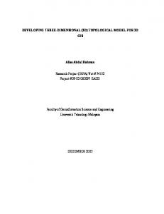
Fig. 2. (a) First of the two frames of squares used and initial curves. (b) Computed 3-D motion segmentation. (c) Image motion reconstructed from the 3-D interpretation estimated by our method. (d) Image motion estimated by the Horn–Schunk method. (e), (f) Reconstructed 3-D structure of the planar objects.

[37] for multiple region segmentation, we obtain the following (see Appendix): functional derivatives for the evolution of (17) with corresponding Euler–Lagrange descent equations

For a stable numerical implementation of (18), we use the implicitly by level set formulation. We represent each curve . With the zero level set of a function corresponding to the set , one can the interior of show [25] that, if the evolution of a curve is described by the equation

(18) where the dependence on is left implicit for simplicity, is the mean curvature of , is the exterior unit normal function are defined by to curve , and functions (19)

where is a function defined on , then the evolution of the corresponding level set function is given by

6

IEEE TRANSACTIONS ON IMAGE PROCESSING

Fig. 3. (a) First frame of teddy1 sequence and initial level set. (b) Computed 3-D motion segmentation. (c) Image motion reconstructed from the 3-D variables estimated by our method. (d) Image motion computed with Horn–Schunk method.

In our case, therefore, we obtain the following system of coupled partial differential equations:

(20) where the mean curvature and by

is given by

for such that else. Summary of the Algorithm: Initialize depth and the curves. Repeat

1)

Compute the parameters of motion by least squares (6). 2) Update depth by one iteration of the descent (11). 3) Evolve the curves using one iteration of the level set descent (20). Until convergence. Depth is initialized to that of a fronto-parallel plane. The curves are initialized to circles. Note that the objective functional is decreased at each step of the algorithm. Therefore, the functional being positive, the algorithm converges to a local minimum. Three-Dimensional Interpretation Up to Scale Factor: Methods of sparse 3-D interpretation [7] can recover depth and the translational component of rigid motion

SEKKATI AND MITICHE: CONCURRENT 3-D MOTION SEGMENTATION

7

Fig. 4. Reconstructed 3-D structure of the moving bear (a) with anisotropic smoothing of depth, (b) without anisotropy, and (c) gray scale od depth.

only up to a scale factor. We ask whether a similar result holds for dense interpretation by a variational method such as the one investigated here. Consider a Tikhonov regularization for depth . Let the change of variables in the functional (4), i.e., and reflect a change of scale of and , where is a positive real number. Consider now the three evolution equations of the algorithm, namely, (6), (12), and and (20). Equation (6) is verified by the scaled variables . As for (12), we have the following evolution equation for , after manipulation and simplification: (21) with ables with

. Similarly, (20) is verified by the scaled varireplaced by in the expression of . Therefore,

to any solution obtained with a regularization factor and initial condition , corresponds, with a regularization factor and initial condition , and for any positive real number , a solution with and scaled by . This shows a three-fold nature for : It weighs the contribution of the second term in the objective functional ( has a similar role), converts the unit of this term to that of the first ( has a similar role), and it fixes the scale of depth and the translational component of motion. It is not clear at this point what the effect on scale would be when using boundary preserving functions . IV. EXPERIMENTAL VERIFICATION To validate the approach and its implementation, we ran several experiments on both synthetic and real image sequences.

8

IEEE TRANSACTIONS ON IMAGE PROCESSING

Fig. 5. (a) First of the two frames used and initial curves. (b) Computed 3-D motion segmentation. (c), (d) Reconstructed 3-D structure of the moving blocks.

The results reported here are obtained using only two frames of each sequence. The use of a larger number of frames may improve results. For instance, one can envisage an extension of the formulation to the spatiotemporal domain as was done in [39] for motion detection and tracking. Exact knowledge of the focal length is not critical for the purpose of this study. In our experiments, we set it to 8.5 mm, which is that of common cameras. Depth is initialized arbitrarily to 65 cm. The algorithm is terminated when the computed variables cease to evolve significantly. Reconstructed objects are displayed using gray-level, triangulation-based surface rendering, and anaglyphs of stereoscopic images constructed from the estimated depth. Also shown is the optical flow reconstructed from the algorithm’s output (1), compared to the optical flow computed directly by the Horn–Schunck method, and to ground truth for the examples for which it is available. For proper viewing, optical flow is scaled before display. We show four examples. This first example uses the synthetic Squares sequence which we constructed. The planar background and both planar objects move, one object occluding the other. The occluding object image motion is (1, 1) in pixels, and that of the occluded object is ( 1, 2). The background

motion is (0, 1). The first of the two frames used is shown in Fig. 2(a), along with the initial two curves of segmentation. The final segmentation, the image motion reconstructed from the estimated 3-D variables (1), and the image motion estimated by the Horn–Schunk method are represented in Fig. 2(b)–(d), respectively. The structure of both planar objects are faithfully recovered as shown separately in Fig. 2(e) and (f). We notice, here, that the two squares are computed at approximately the same depth because the term of smoothness of depth is approximately zero in this particular example. The second example uses the teddy1 sequence (Carnegie Mellon Image Database), in which an object (a teddy bear) moves against a moving textured background. The object moves approximately laterally, the background in the opposite direction. Note that the object of this sequence presents difficulties because of large areas of weak spatiotemporal variations as well as small features without texture such as eyes, nose tip, and bow tie. The first of the two frames used, with the initial curve, is shown in Fig. 3(a). The final segmentation is shown in Fig. 3(b). Image motion recovered from the estimated 3-D variables (1) and from the Horn–Schunk method are displayed in Fig. 3(c) and (d). Note that a 3-D fronto-parallel translational motion

SEKKATI AND MITICHE: CONCURRENT 3-D MOTION SEGMENTATION

9

Fig. 6. (a) Gray scale of depth. (b) Ground truth image motion of marbled-block. (c) Recovered image motion from the 3-D in estimated by our method. (d) Image motion computed with Horn–Schunck method.

does not produce a translation in the projection plane [see (1)]. This can be clearly seen in this example. Fig. 4 displays the recorded depth, triangulated and shaded according to a local light source. To show the improvement obtained with anisotropic smoothing of depth (11) in preserving boundaries (eyes, noses, bow tie), the recovered structure is displayed when using anisotropy [Fig. 4(a)] and without anisotropy [(12); Fig. 4(b)]. The estimated depth is shown in gray scale in Fig. 4(c). In this next example, we use the Marbled-block sequence (image database of KOGS/IAKS Laboratory, University of Karlsruhe, Germany). Two blocks are in motion independently against a static background. The larger block moves to the left and slightly up. The other block moves diagonally to the left. Fig. 5(a) shows the first of the two frames used, along with the two curves of the initial segmentation. The blocks cast shadows. Also, the texture of the top of the blocks is identical to that of the background, causing two of the image occluding edges to be very week, not visible at places. For this sequence, depth presents sharp discontinuities at occlusion boundaries. The computed segmentation is displayed in Fig. 5(b). The reconstructed depth of the blocks (triangulated and shaded according to a local light source) are shown in Fig. 5(c) and (d). Note that the edges between the blocks faces are preserved due to the use of anisotropic diffusion on depth. A gray level representation of

depth is also given in Fig. 6(a). The ground truth image motion, the image motion reconstructed from the estimated depth (1), and image motion computed by the Horn–Schunck algorithm, are displayed in Fig. 6(b)–(d), respectively. This last example uses the Robert sequence of real images taken in common, realistic conditions (Heinrich-Hertz Institute image database, Germany). This is a complex sequence of real images of a person moving his head, lips, and eyebrows against a noisy textured background. The head moves backward and slightly to the left. The movements of the eyebrows and lips do not fit the rigid motion assumption when considered with the movement of the head. The sequence is taken under common lighting. There are large areas (hair, cheeks, forehead) with weak spatiotemporal variations. The particularities of this sequence make it a good testbed to show the difficulties faced by, and the limitations of, algorithms to reconstruct 3-D structure from a temporal sequence spatiotemporal variations. Fig. 7(a) shows the first frame of this sequence along with the curve of the initial segmentation. The final segmentation is shown in Fig. 7(b). The image motion reconstructed from (1), and image motion computed by the Horn–Schunck algorithm are displayed in Fig. 7(c) and (d), respectively. The reconstructed depth of the head (triangulated and shaded according to a local light source) is shown in Fig. 7(e), and the corresponding gray

10

IEEE TRANSACTIONS ON IMAGE PROCESSING

Fig. 7. (a) First frame of robert sequence and initial level set. (b) Computed 3-D motion segmentation. (c) Image motion reconstructed from the 3-D variables estimated by our method. (d) Image motion computed with Horn–Schunk method. (e) Reconstructed 3-D structure of the moving head. (f) Gray scale of depth.

scale of depth of the whole scene is shown in Fig. 7(f). The computed segmentation is overall satisfactory although parts of the hair and ears, as well as the lips and eyebrows are affected to the background due to their lack of texture. Also, the reconstructed depth is shallower than in the other examples. This is due to the weak spatiotemporal variations on the image of practically the entire face. Varying the initialization has given the same segmentation and 3-D interpretation. As with the other examples, careful setting of the weights in the functional is necessary since these weights set the relative contribution of the various terms in the functional.

A. Anaglyph Viewing of the Computed 3-D Interpretation We can view the 3-D interpretation of a monocular sequence by viewing an anaglyph of a stereoscopic image constructed from an image of the monocular sequence and the estimated depth for that image. Anaglyphs on paper are best viewed when printed on high quality photographic paper. When viewing on a CRT screen, high resolution and display options for high quality color image rendering offer a clearer impression of depth. In all cases, however, anaglyphs offer a good, inexpensive means of viewing 3-D interpretation results.

SEKKATI AND MITICHE: CONCURRENT 3-D MOTION SEGMENTATION

11

Fig. 8. Color anaglyphs of (a) squares, (b) marbled-block, (c) teddy1, and (d) Robert.

Given an image and the corresponding depth map, we constructed a stereoscopic image using the following simple be the given image. will be one of the two scheme. Let images of the stereoscopic pair and we construct the other be the viewing system representing the image, . Let that of the other (fictitious) camera which acquired , and

is placed to camera. Both viewing systems are as in Fig. 1. by a translation of amount along the X axis. differ from Let a point on the image position array of , correin sponding to a point in space with coordinates . The coordinates of in are , , and . The image of in the image domain of are,

12

IEEE TRANSACTIONS ON IMAGE PROCESSING

according to our viewing system model (Fig. 1)

Therefore (22) (23)

are Because depth has been estimated, coordinates known. Image , which will be the second of the stereoscopic pair, is then constructed as follows: (24) where is the -coordinate of the point on the image positional with coordinate closest to . Alternatively, one array of can use interpolation. However, we found it unnecessary for our purpose here. The anaglyph images constructed for the four sequences are shown in Fig. 8. They are to be viewed with chromatic (red-blue) glasses (common, inexpensive commercial plastic glasses are available). Viewers presented with these anaglyphs experienced a strong sense of depth for all sequences. The 3-D interpretation of the Squares sequence places the two objects at the same depth against a the background because the regularization term for depth vanishes for planar surfaces. The anaglyphs have been generated using the algorithm in [40] (courtesy of E. Dubois, its inventor).

which yields (9). Following the justification in [34] and [37], , are the descent equations with respect to , obtained by simultaneous minimization of the following functionals:

(26) is the set complement of and . Using the generic derivations in [27], [38], the derivative with respect to of the terms of (26) are given by where

V. CONCLUSION We presented a novel method to segment multiple independent 3-D motions and simultaneously infer 3-D interpretation in temporal sequences of monocular images. Both viewing system and viewed objects were allowed to move. The problem was stated according to a variational formulation. The corresponding Euler–Lagrange descent equations led to an algorithm which, after initialization, iterated three consecutive steps, namely, computation of rigid 3-D motion parameters by least squares, depth by gradient descent, and curve evolution by level sets PDEs. The algorithm and its implementation have been validated on synthetic and real image sequences. Viewers strongly perceived depth in stereoscopic images constructed from the scheme’s output. APPENDIX The energy (7) can be written in general form as (25) where functional derivative of

where

. The with respect to

is

which lead to evolution (17) for

,

.

REFERENCES [1] T. Huang, Image Sequence Analysis. New York: Springer-Verlag Berlin Heidelberg, 1981. [2] J. Aloimonos and C. Brown, “Direct processing of curvilinear sensor motion from a sequence of perspective images,” in Proc. IEEE Workshop on Computer Vision: Representation and Analysis, Annapolis, MD, 1984, pp. 72–77. [3] B. Horn and E. Weldon, “Direct methods for recovering motion,” Int. J. Comput. Vis., vol. 2, no. 2, pp. 51–76, 1988. [4] J. Aggarwal and N. Nandhakumar, “On the computation of motion from a sequence of images: a review,” Proc. IEEE, vol. 76, no. 8, pp. 917–935, Aug. 1988. [5] T. Huang and A. Netravali, “Motion and structure from feature correspondences: A review,” Proc. IEEE, vol. 82, no. 2, pp. 252–268, Feb. 1994. [6] O. Faugeras, Three Dimensional Computer Vision: A Geometric Viewpoint. Cambridge, MA: MIT Press, 1993. [7] A. Mitiche, Computational Analysis of Visual Motion. New York: Plenum, 1994. [8] A. Zisserman and R. Hartly, Multiple View Geometry in Computer Vision. Cambridge, U.K.: Cambridge Univ. Press, 2000. [9] B. Horn and B. Schunk, “Determining optical flow,” Artif. Intell., no. 17, pp. 185–203, 1981. [10] G. Aubert, G. Deriche, and P. Kornprobst, “Computing optical flow via variational techniques,” SIAM J. Appl. Math., vol. 60, no. 1, pp. 156–182, 1999. [11] A. Mitiche and P. Bouthemy, “Computation and analysis of image motion: a synopsis of current problems and methods,” Int. J. Comput. Vis., vol. 19, no. 1, pp. 29–55, 1996. [12] J. Mellor, S. Teller, and T. Lozano-Perez, “Dense depth map for epipolar images,” in Proc. Image Understanding Workshop, 1997, pp. 893–900. [13] S. Negahdaripour and B. Horn, “Direct passive navigation,” IEEE Trans. Pattern Anal. Mach. Intell., vol. PAMI-9, no. 1, pp. 168–176, 1987. [14] R. Laganiere and A. Mitiche, “Direct bayesian interpretation of visual motion,” J. Robot. Autonom. Syst., no. 14, pp. 247–254, 1995. [15] R. Chellappa and S. Srinivasan, “Structure from motion: sparse versus dense correspondance methods,” in Proc. Int. Conf. Image Processing, vol. 2, 1999, pp. 492–499.

SEKKATI AND MITICHE: CONCURRENT 3-D MOTION SEGMENTATION

[16] Y. Hung and H. Ho, “A kalman filter approach to direct depth estimation incorporating surface structure,” IEEE Trans. Pattern Anal. Mach. Intell., vol. 21, no. 6, pp. 570–575, Jun. 1999. [17] S. Srinivasan, “Extracting structure from optical flow using the fast error search technique,” Int. J. Comput. Vis., vol. 37, no. 3, pp. 203–230, 2000. [18] T. Brodsky, C. Fermuller, and Y. Aloimonos, “Structure from motion: beyond the epipolar constraint,” Int. J. Comput. Vis., vol. 37, no. 3, pp. 231–258, 2000. [19] H. Longuet-Higgins and K. Prazdny, “The interpretation of a moving retinal image,” Proc. Roy. Soc. Lond. B, pp. 385–397, 1981. [20] G. Adiv, “Determining three-dimensional motion and structure from optical flow generated by several moving objects,” IEEE Trans. Pattern Anal. Mach. Intell., vol. PAMI-7, no. 4, pp. 384–401, Apr. 1985. [21] A. Mitiche and S. Hadjres, “Mdl estimation of a dense map of relative depth and 3D motion from a temporal sequence of images,” Pattern Anal. Applicat., no. 6, pp. 78–87, 2003. [22] H. Sekkati and A. Mitiche, “Dense 3D interpretation of image sequences: A variational approach using anisotropic diffusion,” presented at the Int. Conf. Image Analysis and Processing, Mantova, Italy, 2003. [23] F. Morier, H. Nicolas, J. Benois, D. Barba, and H. Sanson, “Relative depth estimation of video objects for image interpolation,” in Proc. Int. Conf. Image Processing, 1998, pp. 953–957. [24] F. Martinez, J. Benois-Pineau, and D. Barba, “Extraction of the relative depth information of objects in video sequences,” in Proc. Int. Conf. Image Processing, 1998, pp. 948–952. [25] J. Sethian, Level Set Methods and Fast Marching Methods. Cambridge, U.K.: Cambridge Univ. Press, 1999. [26] S. Jehan, M. Gastaud, M. Barlaud, and G. Aubert, “Region-based active contours using geometrical and statistical features for image segmentation,” presented at the Int. Conf. Image Processing, Barcelona, Spain, 2003. [27] G. Aubert and P. Komprobst, Mathematical Problems in Image Processing. New York: Springer, 2002. [28] S. Osher and N. Paragios, Geometric Level Set Methods in Imaging, Vision, and Graphics. New York: Springer, 2003. [29] O. Faugeras and R. Keriven, “Variational principles, surface evolution, PDE’s, level set methods, and the stereo problem,” IEEE Trans. Image Process., vol. 7, no. 3, pp. 336–344, Mar. 1998. [30] H. Sekkati and A. Mitiche, “Joint dense 3D interpretation and multiple motion segmentation of temporal image sequences: a variational framework with active curve evolution and level sets,” presented at the Int. Conf. Image Processing, Singapore, 2004. [31] D. Mumford and J. Shah, “Optimal approximation by piecewise smooth functions and associated variational problems,” Commun. Pure Appl. Math., no. 42, pp. 577–685, 1989. [32] R. Feghali and A. Mitiche, “Fast computation of a boundary preserving estimate of optical flow,” in Proc. Brit. Machine Vision Conf., 2000, pp. 212–221. [33] T. Chan and L. Vese, “An active contour model without edges,” in Proc. Int. Conf. Scale-Space Theories in Computer Vision, Corfu, Greece, 1999, pp. 141–151.

13

[34] A. Mansouri and J. Konrad, “Multiple motion segmentation with level sets,” IEEE Trans. Image Process., vol. 12, no. 2, pp. 201–220, Feb. 2003. [35] A. Mansouri, A. Mitiche, and C. Vazquez, “Image segmentation by multiregion competition,” presented at the Reconnaissance de Formes et Intelligence Artificielle Conf., RFIA-04, Toulouse, France, 2004. [36] C. Vazquez, A. Mitiche, and I. B. Ayed, “Segmentation of vectorial images by a global curve evolution method,” presented at the Reconnaissance de Formes et Intelligence Artificielle Conf., RFIA-04, Toulouse, France, 2004. [37] , “Image segmentation as regularized clustring: a fully flobal curve evolution method,” in Int. Conf. Image Processing, Singapore, 2004, pp. 3467–3470. [38] S. Zhu and A. Yuille, “Region competition: unifying snakes, region growing, and bayes/mdl for multiband image segmentation,” IEEE Trans. Pattern Anal. Mach. Intell., vol. 18, no. 9, pp. 884–900, Sep. 1996. [39] A. Mitiche, R. Feghali, and A. Mansouri, “Motion tracking as spatiotemporal motion boundary detection,” J. Robot. Autonom. Syst., no. 43, pp. 39–50, 2003. [40] E. Dubois, “A projection method to generate anaglyph stereo images,” in Proc. ICASP, vol. III, 2001, pp. 1661–1664.

Hicham Sekkati received the Licence Ès Sciences in physics and the Diplome d’études approfondies (DEA) in automatic and signal processing from the university Mohammed V, Rabat, Morocco, in 1993 and 1994, respectively, and the M.S. degree in telecommunications from the National Institute of Scientific Research (INRS-EMT), Montreal, QC, Canada, in 2003. He is currently pursuing the Ph.D. degree at the INRS-EMT. His research interests are in computer vision and image processing.

Amar Mitiche received the Licence És Sciences in mathematics from the University of Algiers, Algiers, Algeria, and the Ph.D. degree in computer science from the University of Texas, Austin. He is currently a Professor in the Department of telecommunications, Institut National de Recherche Scientifique, Montreal, QC, Canada. His research interests include computer vision, motion analysis in monocular and stereoscopic image sequences (detection, estimation, segmentation, and tracking) with a focus on methods based on level-set PDEs, and written text recognition with a focus on neural networks methods.