of intensity dI is a linear function of the object motion dPo. Under the small motion assumption, dN has only two degrees of freedom (on the plane perpendicular ...
3D Motion Segmentation Using Intensity Trajectory Hua Yang1 , Greg Welch2 , Jan-Michael Frahm2 , and Marc Pollefeys2 2
1 Kitware, Inc. Computer Science Department, University of North Carolina at Chapel Hill
Abstract. Motion segmentation is a fundamental aspect of tracking in a scene with multiple moving objects. In this paper we present a novel approach to clustering individual image pixels associated with different 3D rigid motions. The basic idea is that the change of the intensity of a pixel can be locally approximated as a linear function of the motion of the corresponding imaged surface. To achieve appearance-based 3D motion segmentation we capture a sequence of local image samples at nearby poses, and assign for each pixel a vector that represents the intensity changes for that pixel over the sequence. We call this vector of intensity changes a pixel “intensity trajectory”. Similar to 2D feature trajectories, the intensity trajectories of pixels corresponding to the same motion span a local linear subspace. Thus the problem of motion segmentation can be cast as that of clustering local subspaces. We have tested this novel approach using some real image sequences. We present results that demonstrate the expected segmentation, even in some challenging cases.
1
Introduction
Motion segmentation has been an active research topic in recent years. Motivated by 2D motion estimation, in particular optical flow work, most of the early approaches to motion segmentation address the problem of segmenting pixels using dense 2D flow fields. For instance, Black and Anandan use robust statistics to handle discontinuities in the flow fields [1]. In layered approaches [2] [3], images are segmented into a set of layers. These methods work on image motion and can not be extended to accommodate 3D motion. Common approaches to 3D motion analysis segmentation are feature-based. They usually aim at clustering feature points according to their underlying motion. Early work includes applying robust statistic methods like RANSAC [4]. Pioneered by Costeira and Kanade’s work, multi-body factorization based methods have been proposed [5] [6] for segmenting independent affine motions. These algorithms use as input a matrix of 2D feature trajectories (sequences of image coordinates of feature points across multiple frames), then use algebraic factorization techniques to cluster the feature trajectories into groups with different motions. One issue with the factorization method is that it assumes independent motion. Recently, to address more complicated scenes that exhibit partially
dependent-motion, [7] [8] propose to solve motion segmentation by clustering the motion subspaces spanned by the feature trajectories. Salient feature is not the only visual cue for analyzing motion. Researchers have widely used dense appearance measurements for tracking 3D motion. Traditional 3D appearance-based methods usually assume a 3D texture mapped model of the target object that is acquired off-line [9] [10] [11] or on-line [12]. The region of interest in the image is precisely initialized by an external (usually manual) method and is assumed to be accurately predicted by projecting the 3D model into the image space using the estimated motion. In addition to 3D models, researchers have also explored acquiring parametric representation of the scene appearance directly from training image samples. For instance, Murase and Nayar proposed an eigenspace-based recognition method and demonstrated tracking 1D motion of a rigid object [13]. Deguchi applied a similar eigenspace representation to simultaneously track rigid motions of the target camera and object [14]. Most image-based approaches require a large number of training images. Recently, a differential approach has been proposed to tracking 3D camera motion in complicated scenes without any prior information [15]. However, it made the assumption of a static scene. We believe that by providing semantic information about the underlying scene motion, a dense appearance-based 3D motion segmentation method could be valuable to image-based methods. Moreover the model-based methods may also benefit from motion segmentation, as it provides an alternative to the manual initialization process to locate the target. Compared to the prosperous research in feature-based techniques, dense (perpixel) 3D motion segmentation is to a large extend unexplored. To our knowledge, only one effort has been made to address dense 3D motion segmentation [16]. In that approach, image regions are segmented using optical flow, or more exactly, covariance-weighted optical flow approximated using spatial and temporal intensity derivative measurements. To address the noisy flow estimate, the authors proposed to compute a covariance-weighted flow-field using intensity measurement, under the assumption of brightness constancy [17]. A covariance matrix flow-field matrix is formed by stacking row vectors of transformed 2D flows of all image regions across multiple frames. Motion-based segmentation is achieved by factorizing the covariance-weighted flow-field matrix into a motion matrix and a shape matrix. Then regions with same motion are grouped by computing and sorting a reduced row echelon form of the shape matrix. In this paper, we will present an approach to clustering individual image pixels associated with different 3D rigid motions. Similar to [16], our method is based on the observation that the image measurements captured from different perspectives across multiple frames span a linear subspace. However, instead of 2D flow fields we use the less noisy 1D pixel intensities as the input measurements. Specifically, we introduce the notion of the pixel intensity trajectory, a vector that represents the intensity changes of a specific pixel over multiple frames. Like the 2D feature trajectories, the intensity trajectories of pixels associated with the same motion span a low-dimensional linear subspace. We therefore formulate the problem of motion segmentation as that of clustering local subspaces. Unlike the
flow-based technique, this linear model of the intensity measurements does not require strict brightness constancy. As we will discuss later, it can be extended to accommodate more general cases, such as illumination changes on Lambertian surface under directional lighting. For segmenting motion subspaces, we apply spectral clustering to the intensity trajectories. This classification technique addresses some issues of direct matrix factorization, such as the noise-sensitivity [18] and the difficulty in handling partially dependent motion [19].
2 2.1
Clustering motion subspaces Intensity trajectory matrix
We begin our discussion in scenes with constant uniform illumination. In this case, the image intensity can be represented as a function of the pose P of the corresponding imaged surface patch in the camera viewing space. Let P = [x, y, z, α, β, γ] represents the relative pose between the object and the camera. Let I(u, P ) be the image intensity, or a filtered version of the image intensity, of a pixel u = [ux , uy ] captured at a pose P . Using the brightness constancy equation, we can compute a local linearization of the intensity function using a Taylor expansion. Let dP be the 3D motion. If dP is small, namely image motion caused by dP is sub-pixel, the change of intensity dI can also be locally linearized as ∂I dI = I(u, P + dP ) − I(u, P ) = dP (1) ∂P Consider acquiring a reference image I0 at pose P0 , and a sequence of f images Ii at nearby poses Pi , and then computing f difference images dIi = Ii − I0 (i = 1, ..., f ). Next assign each pixel an f -vector that represents its intensity changes over the f different images corresponding to the motions dPi . We call the f -vectors of intensity changes dI = [dI1 , dI2 , ..., dIf ] pixel intensity trajectories (as oppose to the 2D feature trajectories). Next construct an intensity trajectory matrix W that combines the intensity trajectories of all n image pixels. The rows of W represent difference images, and its columns represent pixel intensity trajectories. ¯ ¯ ¯ dI1,1 ... dI1,n ¯ ¯ ¯ ¯ ¯ W = ¯ ... . . . ... ¯ ¯ ¯ ¯ dIf,1 ... dIf,n ¯ 2.2
Motion subspaces
Consider a scene with a single 3D rigid motion. Using equation (1), W can be decomposed into two matrices: a motion matrix M of size f × 6 and an intensity Jacobian matrix F of size n × 6 as follows. W = MFT
(2)
¯ ¯ ∂I ¯ ∂P 1,1 ¯ F = ¯¯ ... ¯ ∂I ¯ ∂P n,1
... .. . ...
¯ ¯ ¯ ¯ dP1,1 ¯ ¯ .. ¯¯ , M = ¯ .. ¯ . . ¯ ¯ ¯ ∂I ¯ dPf,1 ¯ ∂P n,6 ∂I ∂P 1,6
¯ ... dP1,6 ¯¯ . ¯ .. . .. ¯¯ ... dPf,6 ¯
If the scene texture and the motion are non-degenerate, M and F are of rank 6. Thus the intensity trajectory matrix W is at most rank 6 (less for degenerate cases). In other words, the intensity trajectories of pixels associated with a single 3D rigid motion span a linear subspace, whose rank is less than or equal to 6. Now consider the intensity trajectory matrix when the scene contains k different motions. In this case, the image pixels belong to k groups. Each group corresponds to the scene surfaces undergoing the same motion. To demonstrate the structure of the W matrix, we assume a certain permutation matrix Λ such that W = |W1 , W2 , ..., Wk | Λ¯ ¯ ¯ ¯ F1T ¯ ¯ T ¯ ¯ F 2 (3) ¯ ¯ = |M1 , M2 , ..., Mk | ¯ ¯Λ . .. ¯ ¯ ¯ ¯ ¯ FkT ¯ Wi = Mi FiT
(i = 1, 2, ....k)
(4)
where Mi and Fi are the motion matrix and intensity Jacobian matrix for the i-th group, and Wi is the concatenation of pixel intensity trajectories of pixels in that group. Again rank(Wi ) ≤ 6. From Equations (3) and (4), we can see that the intensity trajectories captured in a scene with k rigid motions can be clustered into k groups, which span k linear subspaces of rank less than 6. This indicates that motion segmentation can be achieved through subspace clustering. 2.3
Motion subspaces under directional illumination
The previous analysis assumes brightness constancy. In this section, we will show that such a constraint can be relaxed to accommodate scenes with Lambertian objects and constant directional light sources. Consider a scene that consists of m light sources with directions Li and magnitudes li (i = 1...m), and a 3D point p on a convex object with surface normal N and albedo λ. If we denote the incidence angle, the angle between the ray from light source i and the surface normal at p, to be θi , the intensity of p can be written as m m X X I= li λ max(Li · N, 0) = li λ max(cos θi , 0) (5) i=1
i=1
Denote the half cosine function as ki = max(cosθi , 0). Its derivative can be written as 3 ½ ∂ki − sin θi − π2 < θi < π2 = (6) 0 otherwise ∂θi 3
i The partial derivative ∂k is unbounded at θi = 0. This discontinuity only affects ∂θi pixels lying exactly on the illumination silhouette. In practice, its effect is usually blurred out by the image low-pass filtering process (see Section 4).
Now let us consider the change of the intensity caused by the motions of the object and the camera. We denote object motion as dPo . Unlike the dP used in previous sections, dPo is defined in the world space. We begin our discussion by assuming a fixed camera. When the object motion consists of nonzero rotational components, the surface normal and the incidence angles will change accordingly. Denote the change of the incidence angle of light source i as dθi . For a small dPo and thus a small dθi , we can apply Taylor extension and represent the change of the pixel intensity dI as a linear function of dθi . dI = λ
m X ∂ki dθi li ∂θi i=1
(7)
From Equation (7), we can see that the change of intensity dI of point p is a linear function of dθi . For fixed distant light sources, the incidence angle θi (i=1...m) is determined by the surface normal N . Therefore, θi is function of N . Under small motion, we can approximate the change of incidence angle dθi as a linear function of the change of the surface normal dN . dθi = arccos(Li · (N + dN )) − arccos(Li · N ) 1 ≈−√ Li · dN = − sin1θi Li · dN 2 2
(8)
1−(Li ·N )
If θi is not zero, it is clear that dθi is a linear function of dN . Notice that θi is zero only when N and Li align with each other. In this case, dN is perpendicular to Li . Using a small angle approximation of sin θ = θ, we have dθi = sin dθi = dN . From Equation (7) and (8), we can see that dI is a linear function of dθi , which is a linear function of dN . Since dN is clearly a linear function of dPo , the change of intensity dI is a linear function of the object motion dPo . Under the small motion assumption, dN has only two degrees of freedom (on the plane perpendicular to N ). Thus the change of intensity dI caused by the change of illumination lies in a 2D subspace. For a fixed camera, the relative motion between the object and the camera dP is the same as dPo . Thus the 2D illumination subspace is embedded in the 6D motion subspace. In more general cases, where both the object and the camera move independently, dP is independent of dPo . The 2D illumination subspace and the 6D motion subspace are orthogonal. Therefore, for a scene with convex Lambertian objects and constant directional light sources, the intensity trajectories of pixels corresponding to the same underlying motion generally span a 8D subspace.
3
Motion segmentation by clustering local subspaces
We have discussed that given a number of local image samples captured at nearby poses (sub-pixel motion), one can construct an intensity trajectory matrix W . The 3D motion segmentation can be formulated as clustering columns of W with respect to their different underlying motion subspaces. The column clustering can be achieved by factorizing the measurement matrix [5] [6] [16]. However, matrix factorization requires the underlying motions
to be independent [19], an assumption often violated in real environments. Recently, researchers have attempted to address partially-dependent motion. Most notably are Vidal and Hartley’s algebraic-based approach [7] and Yan and Pollefeys’s spectral-based approach [8]. A review can be found in [20]. We employ the so called Local Subspace Affinity (LSA) method for clustering motion subspaces [8]. The LSA algorithm is based on local linear projection and spectral clustering. Instead of working directly on the trajectory matrix W , LSA fits a local subspace for each point and constructs a similarity matrix A using the pairwise distances between the local subspaces. Motion segmentation is achieved by spectral clustering of the similarity matrix. The algorithm can be described in four steps: Step 1. Dimension reduction and data normalization: Remove redundant dimensions (usually contributed by noise) by projecting the trajectories from Rf onto a lower dimensional space Rl using SVD. Then normalize these l-vectors onto a unit hyper-sphere. Step 2. Local subspace estimation: For each projected point pi , find its nearest neighbors on the hyper-sphere (not from the image space) and compute a local linear subspace Si of dimension m. Step 3. Similarity matrix construction: Compute the distances (principle angles) between local subspaces, and construct a similarity matrix A, using Equation (9), where θijh is the h-th component of the principle angle vector between two local subspaces Si and Sj . Aij = exp(−
m X
sin2 θijh )
(9)
h=1
Step 4. Spectral clustering: Apply spectral clustering [21] to the similarity matrix A and segment data into k clusters, where k is the number of different rigid motions in the scene. In [8], the dimensions of the projected space l and the local subspace m are automatically determined using a rank detection algorithm to accommodate general unknown motion such as articulated or non-rigid motion. Since this paper only addresses 3D rigid motion, we choose l and m to be 6k and 6 for scenes with uniform lighting or 8k and 8 for directional lighting. There are two potential causes of segmentation error in the above algorithm. First, the neighbors selected in step 2 can be pixels of different subspaces. Second, the selected neighbors may not fully span the underlying motion subspace. In both cases, the local subspace tend to have similar distances to several motion subspaces, and misclassification may occur. To address these issues we have developed a refinement procedure (Step 5). In this procedure, we identify ambiguous pixels by comparing their distances to different motion subspaces, then reclassify them using the spatial continuity of the moving objects. Step 5a.1: For each cluster, compute a global motion subspace spanned by all the pixels belonging to it, using the result from step 4.
Step 5a.2: For each pixel, compute the pixel-to-cluster distance as the distance between its local subspace and its classified global subspace. Then for each cluster, compute the median of the in-cluster pixel-to-cluster distance. Step 5a.3: For each pixel compute the distances between its local subspace and all k global subspaces, normalized by the median in-cluster distance. Compute the ratio of the smallest and the second smallest normalized distances. Classify a pixel as an ambiguous-pixel if its ratio is bigger than a threshold (in all the experiments we set it to be 0.7). Step 5b: For each ambiguous pixel, search for its neighbors in the image space and classify it to the majority class.
4
Acquiring local appearance samples
We have formulated the problem of motion segmentation as clustering linear subspaces spanned by pixel intensity trajectories. The pixel intensity trajectories are computed from a sequence of local image samples. In theory, to span a motion subspace of rank k, we need k + 1 image samples. This number is usually bigger in practice due to the noise issue. Since our subspace formulation is based on linearizing the local appearance manifold (see Equation (1)), the motion of the imaged surface across the sequence needs to be small (within the linear region). It is feasible to acquire sufficient local samples for normally moving objects using commodity imaging devices. First, we can use the common technique of blurring the original image to smooth the appearance manifold. The enlarged linear region can then accommodate larger motion. Secondly, the speed of commodity camera has become high enough to densely sample motion in most practical scenes. For instance, the Point-Gray Flea2 camera can capture at 80 framesper-second at VGA resolution. Moreover, for sampling 3D rigid motion under constant uniform illumination, the number of frames can be reduced by using a small-baseline camera cluster. This technique is based on the dual relationship between the camera motion and the object motion: under the brightness constancy assumption, images of an object captured at a specific pose from different perspectives can be considered as image samples of that object captured at different poses from the same perspective. A prototype of such a small baseline camera cluster is described in [15]. Commercial products are also available. An example is Point-Gray’s ProFUSION, a 5x5 camera array with 12mm spacing.
5
Experiment
To begin we used a camera cluster to capture some intensity trajectories. To do so we implemented a differential camera cluster similar to that used in [15]. Our camera cluster contains four small baseline Point-Gray Flea2 black-and-white cameras. At each frame time, we use the cluster to acquire seven local appearance samples. In addition to the four real samples from the physical cameras, we also generate three simulated images as in [15]. This is achieved by reprojecting one real image to three different synthetic image planes that are generated
by rotating the image plane around its camera center. Simultaneously capturing multiple spatial samples helps to reduce the number of temporal frames. In addition, such a cluster setting can ensure the capture of the full 6D motion subspace for any object in the scene 4 , even if the underlying rigid motion of that object is degenerate within the sequence. Notice that while we use a camera cluster in some of our experiments, for the above reasons, our motion segmentation algorithm is general and is not restricted to a cluster setup. Section 5.2 and section 5.3 show two examples of segmentation using a single physical camera. Our cameras capture images at VGA resolution. However, to accommodate larger motion, we blurred the images to smooth the appearance manifold. In all the experiments, we used a Gaussian filter with σ = 12 to blur the original image and sub-sample the blurred image at a 20-to-1 rate. We ran our motion segmentation algorithm on the sub-sampled image. As a result of the sub-sampling, one pixel in the resulting segmented image corresponds to a 20×20 block in the original image. Note that because the cameras are packed closely in the cluster, some cameras see the lenses of other cameras in the border area. In addition, the blurring process introduces some additional border effects. For these reasons, in our experiments we only processed the inner regions of the images. We tested our algorithm on three real data sets. All of them contain two rigid motions: the camera and one moving object. 5.1
Controlled motion
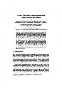
Our first experiment demonstrates motion segmentation in a scene with two controlled rigid motions. To control the motion, we mounted the camera cluster on a 1D translational platform, and a checkerboard on a rail. Between each frame, we shifted the camera and the checkerboard (4mm for the camera, 5mm for the checkerboard) along the directions of their rails. We captured six frames for a total of 42 real and synthetic images, and extracted intensity trajectories from these images. The classification results are presented in Fig. 1. Fig. 1(a) shows the segmentation without refinement. The pixel classification is super-imposed on the original image. Boundary pixels are not processed (they are marked as black). Dark gray and light gray are used to indicate foreground and background pixels, respectively. Ambiguous pixels computed in the refinement process are marked white in Fig. 1(b). The refined motion segmentation results are shown in Fig. 1(c). The misclassification error (number of mis-classified pixels divided by the number of all processed pixels) was 2.5%. Fig. 1(d) shows the similarity matrices permuted using the initial (top) and refined segmentations (bottom). We used the motion segmentation results with the differential tracking method proposed in [15]. At each frame, we used the seven local appearance samples acquired by the differential camera cluster to compute a first-order approximation of the local appearance manifold. When new cluster samples were captured at the next frame time, we then estimated the incremental motion using a linear 4
It only guarantees the motion subspace for each object to be 6D. The motion subspaces of different objects can still be partially dependent.
solver. The estimation results of the controlled motion (restricted to the X-Z plane of the camera coordinate frame) are shown in Fig. 1(e,f). There are five lines in both figures. The “Estimated Whole” line (black, dashed) indicates the motion computed using all of the non-boundary pixels under the assumption of a rigid scene. Using the segmentation results, we estimated different motion components in the scene. The upper and lower pairs of lines respectively represent the real (true) and estimated motion of the checkerboard and the background with respect to the camera. The estimate using all of the pixels (unsegmented) appears to be a weighted average of the two underlying motions, as one would expect, and is clearly wrong for either motion. The result using the segmented pixels appears to be very accurate for the background motion, and reasonably accurate for the foreground motion. Notice that we do not assume scene geometry. While the foreground moving objects in the experiments are planar, the moving backgrounds contain objects with different shapes at different depths.
5.2
Free-form motion
In the second experiment, we used our algorithm to segment two free-form rigid motions—both the camera cluster and the checkerboard were moved by hand. For each frame, we extracted pixel intensity trajectories across a window of 15 adjacent frames. The motion segmentation results over 45 frames are shown in the first row of Fig. 2. Pixels corresponding to the moving checkerboard are marked white. The remaining pixels are classified as background. For a clearer representation, the boundary pixels are excluded. To explore the use of our algorithm in a single camera setting, we ran it again on the above sequence. But this time we only used images captured by one of the four physical cameras and three synthetic rotational cameras. Again, the intensity trajectories are extracted across a window of 15 frames. The results are shown in the second row of Fig. 2. Although only one physical camera is used, the segmentation results are reasonably good.
5.3
Motion segmentation under directional lighting
Our last experiment demonstrates 3D motion segmentation in a scene with directional lighting using a single camera setup. The scene is illuminated with multiple ceiling lights and a directional light source from the left. A person sits on a chair and rotates. All light sources are static and constant. Again, we used images captured by one physical camera and three synthetic rotational cameras. Fig. 3(a) presents the illumination effect of the side light. The segmentation result is shown in (b)-(f). Pixels corresponding to the person and the chair are marked gray. Notice that most of the segmentation error are from pixels on the back of the chair. This is due to the plain texture in that area. In this experiment, the intensity trajectories were extracted from a window of 15 frames.
6
Conclusion and future work
We have presented a novel approach to 3D motion segmentation. Based on a local linear mapping between the changes of the pixel intensities and the underlying motions, we introduced the notion of pixel intensity trajectories, and formulated motion segmentation as clustering local subspaces spanned by those intensity trajectories. We have demonstrated our algorithm using some real data sets. Although we only discuss 3D rigid motion in this work, we believe the analysis can be extended to more general motion such as articulated, non-rigid motion. Just like parameterizing dI into a 6D space for rigid motion (see Equation (1)), for a general motion of rank m, we can map dI into an mD space represented by its motion parameters. In this case the motion vector dP becomes an mD vector. We can still decompose the intensity trajectory matrix W into the motion matrix M and the intensity Jacobian matrix F . All three matrices are of rank m. Thus the intensity trajectories of pixels corresponding to a general motion of rank m span an mD subspace.
References 1. Black, M.J.: The robust estimatoin of multiple motions: Parametric and piecewisesmooth flow fields. Computer Vision and Image Understanding 63(1) (1996) 2. Xiao, J., Shah, M.: Accurate motion layer segmentation and matting. IEEE Conference on Computer Vision and Pattern Recognition (2005) 3. Wang, J., Adelson, E.: Representing moving images with layers. IEEE Transactions on Image Processing 3(5) (1994) 625–638 4. Fischler, M.A., Bolles, R.C.: Random sample consensus: a paradigm for model fitting with applications to image analysis and automated cartography. Readings in computer vision: issues, problems, principles, and paradigms (1987) 726–740 5. Costeira, J., Kanade, T.: A multi-body factorization method for motion analysis. International Conference on Computer Vision (1995) 6. Gear, C.: Multibody grouping from motion images. International Journal of Computer Vision 29(2) (1998) 133–150 7. Vidal, R., Hartley, R.: Motion segmentation with missing data by power factorization and by generalized pca. IEEE Conference on Computer Vision and Pattern Recognition (2004) 310–316 8. Yan, J., Pollefeys, M.: A general framework for motion segmentation: Independent, articulated, rigid, non-rigid, degenerate and non-degenerate. European Conference on Computer Vision (2006) 9. Cascia, M.L., Sclaroff, S., Athitsos, V.: Fast, reliable head tracking under varying illumination: An apporach based on registration of texture-mapped 3d models. IEEE Transactions on Pattern Analysis and Machine Intelligence 22(4) (2000) 10. Malciu, M., Preteux, F.: A robust model-based approach for 3d head tracking in video sequences. Fourth IEEE International Conference on Automatic Face and Gesture Recognition (2000) 11. Moritani, T., Hiura, S., Sato, K.: Real-time object tracking without feature extraction. International Conference on Pattern Recognition (2006) 747–750 12. Zimmermann, K., Svoboda, T., Matas, J.: Multiview 3d tracking with an incrementally constructed 3d model. Third International Symposium on 3D Data Processing, Visualization, and Transmission (2006)
13. Murase, H., Nayar, S.: Visual learning and recognition of 3d objects from appearance. International Journal of Computer Vision 14(1) (1995) 14. Deguchi, K.: A direct interpretation of dynamic images with camera and object motions for vision guided robot control. International Journal of Computer Vision 37(1) (2000) 15. Yang, H., Pollefeys, M., Welch, G., Frahm, J.M., Ilie, A.: Differential camera tracking through linearizing the local appearance manifold. IEEE Conference on Computer Vision and Pattern Recognition (2007) 16. Zelnik-Manor, L., Machline, M., Irani, M.: Multi-body factorization with uncertainty: Revisiting motion consistency. International Journal of Computer Vision 68(1) (2006) 27–41 17. Irani, M.: Multi-frame correspondence estimation using subspace constraints. International Journal of Computer Vision 48(3) (2002) 173–194 18. Gruber1, A., Weiss, Y.: Incorporating constraints and prior knowledge into factorization algorithms - an application to 3d recovery. Lecture Notes in Computer Science 3940 (2006) 151–162 19. Kanatani, K.: Motion segmentation by subspace separation and model selection. International Conference on Computer Vision (2001) 586–591 20. Tron, R., Vidal, R.: A benchmark for the comparison of 3d motion segmentation algorithms. IEEE Conference on Computer Vision and Pattern Recognition (2007) 21. Ng, A., Jordan, M., Weiss, Y.: On spectral clustering: Analysis and an algorithm. Advances in Neural Information Processing Systems (2001)
(a)
(b)
(c)
Motion estimation of X translation
Motion estimation of Z translation
35
25
Estimate Whole Real Back Estimate Back Real Front Estimate Front
30 translation (mm)
translation (mm)
30
35
20 15 10 5 0 1
(d)
25
Estimate Whole Real Back Estimate Back Real Front Estimate Front
20 15 10 5
2
3
4
5
6
0 1
2
3
4
frame
frame
(e)
(f)
5
6
Fig. 1. Motion segmentation and tracking results for a controlled sequence. (a) Segmentation results before refinement. (b) Segmentation results with ambiguous-pixels. (c) Segmentation results after refinement. (d) Similarity matrices before (top) and after (bottom) refinement. (e) and (f) Motion estimation of X translation. (f) Motion estimation of Z translation.
(a)
(b)
(c)
(d)
(e)
(f)
Fig. 2. Segmenting free-form rigid motions across a sequence of 45 frames. The checkerboard and the camera were moved by hand. Images (a)-(c) show the results on segmenting image sequences captured by a camera cluster. Images (d)-(f) show the results on segmenting image sequences captured using a single camera.
(a)
(b)
(c)
(d)
(e)
(f)
Fig. 3. Motion segmentation in a scene with directional lighting across 40 frames. A person was sitting on a chair rotating; the camera were moved by hand. (a) An image from the original sequence showing the person was illuminated by a directional light source from the left side. (b)-(f): Segmentation results on 5 frames from the sequence.