Bre79] and RLF Lei79], to sophisticated search strategies, e.g. simulated annealing Joh91] or tabu search Her87]. Nevertheless, such algorithms usually perform ...
Concurrent Algorithm Development and Software Implementation Strategies and an Application to Graph Coloring� Darko Kirovski and Miodrag Potkonjak Computer Science Department, University of California, Los Angeles
Abstract Algorithm implementation has been commonly addressed separately from the algorithm development process. Moreover, implementation of algorithms has been assumed to be cumbersome, but straightforward process. To show that concurrent algorithm development and implementation may often result in boosting the performance of an algorithm or a synergy of algorithms, we have developed a set of guidelines for algorithm development and implementation. To demonstrate the e�ectiveness the approach, we have applied these techniques to the well-studied problem of graph coloring. The application of the algorithm development and implementation guidelines has emerged a new hybrid algorithm for graph coloring. The ideas that have had crucial impact on algorithm's performance are: successive reduction of the problem space (coloring successively one independent set of vertices at a time), global search for the most-constrained independent set and its computationally inexpensive objective function computation, early coloring of most-constrained vertices in a way that the remainder of the graph is least-constraining, reuse and locality exploration of intermediate solutions, search timing management, iterative solution improvement using lottery-scheduling, and once the software was written, optimization of execution bottlenecks and statistical determination and validation of all program parameters. The algorithm has been tested on a number of real-life examples and graph models which correspond to instances frequently encountered in VLSI CAD. We have found that hard-to-color real-life examples exist, especially in domains where problem modeling results in denser graphs. We have de ned a novel graph model which has a single optimum coloring. Our algorithm has been tested against this provably hard-to-color class of graphs. Extensive experiments have shown that in many instances the algorithm has outperformed all other implementations reported in literature both in solution quality and search run-time. � A preliminary version of parts of this manuscript has been published at the 1998 IEEE/ACM Design Automation
Conference.
1
1 Introduction The ever-increasing amount of resources encountered in contemporary designs with exponentially ascending complexities impacts optimization intensive development, compilation, and fabrication strategies. Since many problems related to resource sharing can be modeled as graph coloring, its importance is selfevident. Possible applications include register assignment, cache line coloring, logic minimization, circuit testing, operations scheduling [Cou97]. Graph coloring is an NP-complete problem [Gar79]. Previous work shows that so far algorithm development was focused on establishing a single heuristic expected to provide exceptional results on all instances. The reported algorithms range from greedy constructive methods, such as DSATUR [Bre79] and RLF [Lei79], to sophisticated search strategies, e.g. simulated annealing [Joh91] or tabu search [Her87]. Nevertheless, such algorithms usually perform well only on small subset of graph model classes or real-life examples. For example, Johnson et al. [Joh91] simultaneously employed three distinct simulated annealing graph coloring techniques: Kempe Chain, Fixed-K , and Penalty Function annealing, and one multivariant successive augmentation XRLF algorithm on a set of various graph models. All implementations resulted in relatively low-quality solutions on some instances. Recently, Coudert proposed a set of exact algorithms for graph coloring based on the knowledge of the maximum clique in a graph [Cou97]. Statistically, such reduction of a hard problem onto another hard problem is not a good problem solving strategy especially when the reduction encompasses nding a maximum clique in a graph, a problem that has been suggested, due to its di�culty, to hide information in some cryptographic protocols [Jue96]. Coudert applied his algorithm on a large set of real-life examples. However, he did not provide experimental results for most graph classes which correspond to di�cult optimization problems. Complex problems such as graph coloring, require extensive exploration of the problem solution space. Deployment of a single search or constraint strategy usually leads to a limited adaptibility to particular problem topologies. Moreover, nding strategies that meet search quality requirements for a large number of problem topologies is an extremely hard task. We have developed a new algorithm for graph coloring which outperforms all algorithms reported in literature with respect to both solution quality and search run-time. In this paper we describe the key algorithm and software development ideas that had crucial impact on the algorithm's performance: successive reduction of the problem space (coloring successively one independent set of vertices at a time), global search for the most-constrained independent set and its computationally inexpensive objective function computation, early coloring of most-constrained vertices in a way that the remainder of the graph is least-constraining, reuse and locality exploration of intermediate solutions, intelligent search timing management, iterative solution improvement post-processing using lottery-scheduling, and once the software was written, optimization of the execution bottlenecks and statistical determination and validation of all parameters in the program. 2
The guidelines that have driven our concurrent algorithm development and implementation have been generalized for a subset of NP-hard problems (e.g. graph partitioning and feedback arc set). The algorithm has been well tested on a number of real-life examples and graph models which correspond to real-life instances frequently encountered in VLSI CAD. We have found that hard-to-color real-life examples exist especially in domains where problem modeling results in denser graphs. We have de ned a novel graph model which has a single optimum coloring. We have tested the algorithm's performance against this provably hard-to-color class of graphs. Extensive experiments have shown that in many instances the algorithm signi cantly outperformed all other implementations reported in literature both in solution quality and search run-time.
2 Related Work In this section the related work in both theoretical and applications domain is presented. Exact graph coloring is with contemporary computing systems possible up to a certain bound on the number of vertices and edges. Various techniques for exact coloring have been developed which try to explore graph's properties in order establish upper bounds and therefore to restrict the solution search space. Experiments show that the best exact techniques are based on the approach developed by Brown [Bro72]. His technique was modi ed by Brelaz [Bre79] and nally the modi cation was improved by Peemoeller [Pee83]. Recently, Coudert presented a set of new exact algorithms based on the knowledge of the maximum clique in a graph [Cou97]. The non-exact algorithms found in literature are driven either by constructive or iterative improvement heuristics. The constructive class of algorithms colors vertices in an order determined by examining properties of the uncolored part of the graph. The simplest constructive algorithm for graph coloring is the "sequential" coloring algorithm (SEQ). Vertices are sequentially traversed and colored with color having the lowest index not used by the already colored neighboring vertices. The worst case bound of this algorithm has been determined to be: O(V � ( logloglogV V )3 ) � �(G) where �(G) is the optimum number of colors and V is the number of vertices. Variety of algorithms outperform SEQ. The current best guaranteed performance algorithm is devised by Halldorson [Hal93]. It guarantees to use no more than log n) ) � �(G) colors. Also a number of constructive heuristics has been developed which sigO( n�(log log n ni cantly outperform SEQ on the average. The most widely used are DSATUR by Brelaz [Bre79] and Recursive Largest First (RLF) by Leighton [Lei79]. In DSATUR the next vertex to color is selected depending on the number of neighbor vertices already colored (saturation degree) where priority is given to vertices with higher saturation degree. Leighton's algorithm colors the vertices sequentially one color class at a time. The algorithm tries to color with each color maximum number of vertices. However, the problem of nding the maximum independent subset in a graph is also intractable ([Gar79], GT20, p.194). Therefore, a heuristic is employed which selects the next vertex to join the current color class 2
3
3
as the one with the largest number of neighbors already assigned to that independent subset. The rst vertex in each independent subset is recommended to be the one with maximum cardinality of incident edges. Best case implementation for both, RLF and DSATUR heuristics results in O(n3 ) running time which makes them ine�cient for coloring large graphs. There exist several di�erent approaches how to utilize the paradigm of iterative improvement in solving the graph coloring problem. Basic model of all iterative improvement schemes probabilistically generates new solutions trying to improve the current best memorized solution. One search strategy, tabu search, was suggested for graph coloring by Hertz and de Werra [Her87]. Another approach, simulated annealing, was rst used for graph coloring by Morgenstern and Shapiro [Mor86]. Di�erent simulated annealing approach was devised by Chams, Hertz, and de Werra [Cha87]. Survey of three highly optimized simulated annealing algorithms was reported along with extensive experimental results by Johnson et al. [Joh91]. Best results up to date were reported for modi ed RLF algorithms which utilize knowledge of the graph's topology in order to establish with exceptional colorings. Such algorithms were implemented by Bollobas and Thomason [Bol85], Johnson et al. [Joh91] and lately by Morgenstern [Mor94]. An e�cient hybrid genetic tabu search algorithm has been developed by Fleurent and Ferland [Fle96]. The standard test example, random V = 1000 vertex graph with p = 0:5 probability of edge existence, averaged 86.9 colors for Bollobas and Thomason [Bol85], and 85.5 for Johnson et al. [Joh91]. Bollobas and Thomason required less than an hour on an IBM 3081, while Johnson et al. required 136 hours on a Sequent Balance 21000 single processor multicomputer. Moreover Johnson et al. reported that they obtained 85 graph colorings only on graphs with "slightly less than expected 0.5" probability of edge existence. The recent attacks by both Morgenstern, and Fleurent and Ferland resulted in 84colorings for the G(1000; 0:5) graph. 84-coloring took between 9 and 36 hours on ve Sparc-2s upgraded with 80MHz CPUs for Morgenstern's mix of distributed XRLF [Joh91, Mor94] and simulated annealing based rejectionless Metropolis move selection. The same coloring quality took 41.35 hours on a Sparc-10 workstation for the tabu search genetic algorithm implementation by Fleurent and Ferland [Fle96]. The question that arises, when a random or real-life graph is given, is whether the lower bound on the solution can be determined. There are methods to analyze the lower bound of the chromatic number of a random graph. Lets denote the chromatic number of a graph G with N vertices and p probability of edge existence as �(G(N; p)). Grimmett and McDiarmid [Gri75] have proved that for a xed probability p the chromatic number �(G(N; p)) satis es: 2 logNd N (1 + O(1)) � �(G(N; p)) � logNd N (1 + O(1)), where d = 1?1 p . Luczak [Luc91] gave an explanation of the asymptotical behavior of the chromatic number when N ! 1 and p ! 0. Then, the chromatic number is bounded within: Np
� Np (1 +
2 log
log log log
Np?1 Np 30�log log Np Np ) � �(G(N; p)) � 2�log Np (1 + log Np ).
We restrict the related work in the graph coloring application domain to VLSI CAD and software 4
synthesis optimization problems. Variable to register assignment problem was treated for the rst time as a graph coloring problem by Chaitin et al. [Cha82]. Other methods for spill code minimization and optimal register assignment are presented in [Cho84, Bri94]. In the cache line coloring problem, program code reordering at link and compile time is performed in order to minimize the number of dynamic cache misses. Bershad et al. have proposed dynamic address remapping for avoiding con ict misses in large direct-mapped instruction caches [Ber94]. In VLSI CAD many problems at all levels of system synthesis can be modeled as graph coloring. Well known problems of resource assignment and static scheduling have been modeled as graph coloring [Kra90, Spr91, Jai93]. Combinational logic test matrices have been developed using graph coloring techniques [Bus95]. Wiring test diagnosis [Che90] and functional logic manipulation [Wan92] can be also modeled as graph coloring.
3 Graph Models The performance evaluation and validation of a graph coloring algorithm is strongly dependent on the benchmark graph topologies. In order to position properly our experiments and the development strategy, in this section we describe the key graph models used to generate the graph instances for our statistical validation mechanisms. The graphs generated using these models were used to determine and evaluate the algorithm in coordination with a large number of real-life examples. We used several diverse graph models: random, geometrical, k-cooked, and uniquely k-cooked graph model. One of the standard test models for graph coloring heuristics is the random graph model denoted as R(V; p). In the notation V is the number of vertices in the graph and p is the probability that a particular edge in the graph exists. The geometric model G(V; d) is used since it has the locality properties as many real-life instances. Geometric graphs are constructed in the following way. In a xed square area a set of V random points is placed. Circles of radius d centered at each of the random points are drawn. A point corresponds to a vertex in the graph, while an edge is created whenever the circles of two edges overlap. The range of the estimated colorability does not assure the algorithm developer in the quality of the proposed algorithm. One class of graphs can be built in such a way that graph's minimal colorability is guaranteed. Such graphs are called k-cooked graphs and are denoted as K (V; p; k). In the notation, V is the number of vertices, p is the probability that a particular edge in the graph exists, and k is the minimum number of colors which is guaranteed to color the graph. The k-cooked graphs in this work were generated using a procedure as presented in Figure 1. Initially k vertices are colored in k distinct colors and a clique is created among them. The remaining vertices of the graph are randomly colored using k colors. Pairs of vertices are then randomly generated and if the vertices in each pair are not colored with the same color, an edge between them is created. This procedure is repeated until the number of edges in the graph is equal to p � V �(V2 ?1) . 5
K-Cooked graph generation:
Generate V vertices Randomly color all vertices with k colors Select one vertex of each color and create a clique among those vertices Number of Edges = k�(k2?1) Repeat
Select randomly two nodes Vi and Vj If an edge which connects Vi and Vj does not exists and Vi and Vj are colored with di�erent colors Create edge EVi ;Vj Number of Edges = Number of Edges + 1 V �(V ?1) until Number of Edges < p � 2
Figure 1: Pseudo-code for k-cooked K (V; p; k) graph generation.
3.1 A Novel Class of Uniquely Colorable -cooked ( K
S V; p; k
) Graphs
One way to provide a hard benchmark is to guarantee that there exists only one solution to the problem. The possibility that a graph has a unique solution has been studied by Bollobas [Bol78]. He proved that a graph of vertex cardinality V is uniquely k-colorable if its minimal degree, �(G) is greater than V � 33��kk??25 . For a 1000 node graph G and 85-colorability this formula guarantees unique solution when the minimal degree �(G) > 992. Thus, graphs are guaranteed to be uniquely colorable only for very dense topologies. Create V vertices Select a set S of k vertices, color them into k distinct colors and create a clique among them Repeat until all vertices are not colored Delete one random vertex Vr from S Let the color of Vr be kr Select one of the uncolored vertices Vi and add edges between Vi and all vertices in S Color Vi with kr and add it to S Let the vertex with maximum number of dissecting edges has MAX edges For each vertex Vi Repeat MAX ? NumberOfEdges(Vi ) times Select randomly an vertex Vj colored with di�erent color than and create an edge E Vi ;Vj between them V �(V ?1) Repeat until Number of Edges < p � 2 Select randomly two nodes Vi and Vj If an edge which connects Vi and Vj does not exists and Vi and Vj are colored with di�erent colors Create the edge EVi ;Vj Number of Edges + 1
Figure 2: Pseudo-code for a uniquely colorable k-cooked S (V; p; k) graph generation. 6
The pseudo-code used to create uniquely colorable k-cooked graphs is presented in Figure 2. The procedure that uniquely colors the graph rst selects a set of k vertices. Then it creates a clique among them. After deleting one vertex from the set, it selects an uncolored vertex, colors it with the color of the deleted vertex, creates edges between the uncolored and all other edges remaining in the set and nally adds the uncolored vertex into the set. The procedure of deleting and adding nodes repeats until all nodes are colored. Note that the procedure up to this point adds exactly k + (V ? k) � (k ? 1) edges. For a 80-colorable 1000 vertices graph S (1000; 0:5; 80) 14.57% of the total number of edges are used in order to create the net of cliques which guarantees a single 80-color solution. 2
2
1
5
1
5
4
6
4
6
3
3 (a)
(b)
2
2
1
5
1
5
4
6
4
6
3
3
(c)
(d)
Figure 3: An example how single solution 3-cooked graph is created. An example of how a single solution 3-cooked graph is created, is depicted in Figure 3. First a clique is created among vertices 1, 4, and 3. Then node 3 is deleted from the set S . Node 2 is colored with the color of node 3 and a clique among 1, 2, and 3 is created. The same set of tasks is performed when nodes 5 and 6 are colored with the color of nodes 1 and 4 and connected to nodes 2 and 4, and 2 and 5 respectively. After creating the net of cliques additional random edges are added (dotted lines). Since 7
at any time the newly selected vertex can take only one color (the one of the deleted vertex), the graph has only one solution. If another solution exists than the vertex that could be colored in another color would have another choice of selecting a color.
4 The New Approach In this section the problem is de ned and the proposed algorithm is described in detail. Also, an insight into the statistical determination and validation of the key parameters in the algorithm is provided. The problem can be de ned using the following standard Garey-Johnson format [Gar79]:
PROBLEM: GRAPH K -COLORABILITY INSTANCE: Graph G(V; E ), positive integer K � jV j. QUESTION: Is G K -colorable. i.e., does there exist a function f : V ! 1; 2; 3; ::; K such that f (u) = 6 f (v) whenever u; v 2 E ?
Graph coloring is an NP-complete problem. Particular instances of the problem which can be solved in polynomial time are listed in [Gar79]. For instance, graphs with maximum vertex degree less than four, and bipartite graphs are guaranteed to be colored in polynomial time. In the general case when K > 2 the problem remains to be NP-hard. We introduce two new distinct graph coloring algorithms and propose their hybrid as a champion algorithmic solution to the graph coloring problem. The rst algorithm is a successive augmentation of a global probabilistic most-constrained least-constraining RLF (lmXRLF). The second one is a lottery-scheduling-driven iterative improvement (lsII) algorithm. The hybrid uses the lmXRLF algorithm to reduce the solution search space until an experimentally determined graph size checkpoint. Then the lsII algorithm iteratively improves the solution until the user stops the search for improvement.
4.1 lmXRLF Reduction of the problem solution space is essential in fast solving of problems with large domains such as graph coloring. The lmXRLF algorithm performs an e�cient problem reduction by coloring early the most-constrained vertices in a way that the remainder of the graph is least-constraining. Therefore, the remaining vertices in the graph after each color assignment are expected to establish a graph coloring subproblem quantitatively and qualitatively easier to solve than the one in the previous step. Successive augmentation of the described technique evolves into a complete lmXRLF algorithm. The cost function that quanti es the vertex constraints is a factor that has crucial impact on the algorithm performance. We have determined experimentally the most-constrained and least-constraining objectives of this search. The pseudo-code of the algorithm is presented in Figure 4. In the rest of this subsection we describe the lmXRLF algorithm and the accompanying algorithm development and implementation guidelines in detail. 8
Color = 0 Repeat
Color = 0 then CANDIDATES = F � GLOBAL ertices2 ) CANDIDATES = GLOBAL � (1 ? NumberOfColoredV V ertices2 Generate a random independent subset S and add it to the list of solutions with largest objective costs ListOfBestSolutions Repeat CANDIDATES times Delete randomly vertices from S until at least one vertex does not have a colored neighbor (not counting the deleted ones) Add randomly vertices which do not have colored neighbors into S If ObjectiveF (S ) > Min(ObjectiveF (ListOfBestSolutionsi )); i = 1::F Add S to the list (the worst objective-e�cient solution is discarded) For each independent subset S in the ListOfBestSolutions If
Else
Repeat
S+ = S
LOCAL times S� = S Delete randomly vertices from S � until at least one vertex does not have a colored neighbor (not counting the deleted ones) Add randomly vertices which do not have colored neighbors into S � If ObjectiveF (S �) > ObjectiveF (S +) then S + = S � S = S+ until there is at least one improvement For each vertex Vi 2 Max(ObjectiveF (ListOfBestSolutionsi ); i = 1; ::; F ) COLOR Vi with Color Discard Vi from further color consideration Delete all solutions S 2 ListOfBestSolutions which have at least one common vertex with Max(ObjectiveF (ListOfBestSolutionsi ); i = 1; ::; F ) Color = Color + 1 until there are uncolored vertices Repeat
Figure 4: Pseudo-code for the graph coloring algorithm.
Solution Space Reduction. The outermost loop of the algorithm drives the search for the most
objective-e�cient independent subset. Once the underlying search returns the subset, all vertices in the independent set are colored with the next available color and deleted from the graph. The described graph reduction is unchangeable, i.e., deleted vertices are not revisited. The objective function that decides the independent set selection was experimentally determined and validated on a set of examples described in Section 5. The objective function found to perform the best on a set of benchmarks is:
ObjectiveF (S ) = PV 2S (NON (V ) � PU 2Neighbor V NON (U ) ) 2
(
)
3
where S is the evaluated independent subset, function Neighbor(V ) returns the set of vertices adjacent to V , and function NON (V ) returns the number of vertices adjacent to V . Thus, vertices found to have large number of incident edges as well as neighborhood with large number of neighbors are treated as constrained. Finding a set of vertices which has the largest accumulated sum of constraints corresponds to the INDEPENDENT SET problem which is also an NP-complete problem [Gar79]. 9
Local Computation of Objectives. Very important property of the objective function is its
local computation and usage of simple search operations such as remove node and add node from/to the current independent set. Local cost computation means that the objective function is not computed over the entire graph, but only over the included/excluded nodes in the new independent set. This approach enables fast independent subset evaluation and boosts the number of independent sets considered in the search. Integer squares and cubes are precomputed which enables avoidance of multiplications in the implementation. Probabilistic Search of the Solution Space. The search for the most objective-e�cient independent subset is performed in the following way. The algorithm rst creates a random initial independent set. Then it iteratively randomly deletes vertices until there exists at least one node in the graph not adjacent to the remaining vertices in the set. Among the uncovered vertices, a subset is randomly selected and added to the independent subset. We experimented greedy strategies for vertex exclusion/inclusion but they did not yield any performance improvement over the fully probabilistic search. Besides introducing larger computation delays between generating two independent sets, controlling the convergence of the greedy probabilistic search strategies is time-consuming and highly sensitive to graph topologies [Joh91]. On the other hand, fully probabilistic search showed unexpectedly good results for all experimented instances. Locality Exploration. During the global problem reduction search, at each step a number of independent subsets is generated. The search is terminated when GLOBAL successive randomly generated independent subsets do not yield any objective improvement. Due to the randomized search, the locality of the most objective-e�cient independent subset is searched extensively in order to nd better slightly di�erent solution. While searching locally, LOCAL number of independent subsets are generated starting from the solution returned by the global search. The nal version of the algorithm performs the local search in recursive fashion until it is stuck in one of the solution space local minima. Maintaining a Pool of Intermediate Solution. During the search for the most objectivee�cient independent subset a set of independent set candidates is generated. When an extensive search is performed, candidates may involve disjoint color classes. In order not to discard the solutions which may be objective-competitive and most probably not reachable in the following search for the next color class, a list of F most objective-e�cient solutions is maintained throughout the search. When the search is stopped and the best independent subset is colored and deleted from the graph, all other independent subsets in the list are checked for mutual vertices and if conjunctive deleted from the list. Hopefully, some independent subsets present good starting points for the next iteration of the search. Search Time Distribution. Finally, since the rst search is handicapped due to lack of previous search results, the number of search iterations is adjusted to the number of solutions available from previous searches and the cardinality of the remaining graph. For the rst color class F � GLOBAL candidates are generated. For every succeeding color class the number of generated candidates during 10
ertices ). Therefore, the program search time is global search equals GLOBAL � (1 ? NumberofColoredV V ertices managed in such a way that di�cult to nd subsets in the beginning of the search are given longer search time-outs. 2
2
(a)
(b)
(c)
(d)
(e)
Figure 5: Example how randomized independent subsets are created. An example, how the search is performed is presented in Figure 5. The black vertices represent the elements of the independent subset. Shaded vertices represent neighbors to the elements of the independent subset. In Figure 5(a) a random node is added to the rst independent subset. In Figure 5(b) the independent subset is completed by adding another vertex (pointed with arrow). In Figures 11
5(c) and (d) another two independent sets are created by discarding (outgoing arrows) and adding (ingoing arrows) vertices into the independent set. Out of the three independent subsets the one in Figure 5(c) is selected as the best one and it is colored with the rst color. All vertices and their dissecting edges are discarded and the graph that remains to be solved is depicted in Figure 5(e). The remaining graph can be colored obviously with two colors. The nal solution yields optimum three colors. The main disadvantage of the described algorithm is the fact that it does not allow search backtracking. Once colored, each vertex is permanently excluded from the graph. It is also hard to establish an objective function that describes the desirability of selecting a particular independent set relatively small with respect to the vertex cardinality of the entire graph (characteristic for extremely dense graphs). For example, the cardinality of most independent subsets of a G(1000; 0:9) graph is four. Evaluating four element independent subsets with respect to the rest of the 1000-node graph is di�cult.
4.2 lsII As described in the previous subsection, there exist instances where iterative solution improvement is required. Many techniques have been developed that exploit probabilistic heuristic-driven solution covergence such as: simulated annealing [Joh91], tabu search [Her87], etc. The main quality of these algorithms is the ability to discard existing and set new color classes. Probabilistic search with controlled greed is used to traverse the solution space. Best solutions are memorized and successive trials are conducted in order to improve the best memorized solution. At any time during the search, the vertex selection and coloring is non-deterministically greedy, i.e. slight probability of traversing towards worse solutions always exists. The main disadvantage of employing such algorithms is the fact that they do not have xed run-times. Moreover, the run-times for obtaining a solution may di�er substantially from one graph to another of the same cardinalities. Finally, the probabilistic parameters, such as annealing rate, are very di�cult to establish and greatly vary depending on the graph topology [Joh91]. We have developed a new iterative improvement algorithm for graph coloring. The lsII algorithm tries to color the graph with xed K number of colors. The graph is initially colored randomly using the K colors. Unfortunatelly, such coloring usually yields incorrectly colored vertices. Therefore, incorrectly colored vertices are considered for recoloring using a greedy heuristic and the lottery-scheduling paradigm for vertex and color selection probability distribution [Wal94]. The recoloring step is iterated until feasible coloring is found. The algorithm is described using the pseudo-code in Figure 6. Each recoloring step consists of two phases. In the rst phase for each incorrectly colored vertex an objective is assigned describing the vertex' constraint. One incorrectly colored vertex is selected probabilistically for recoloring in such a way that vertices with higher constraints are given proportional priority in the lottery-scheduling driven probabilistic selection. As an objective function to quantify the vertex constraint we used the number of adjacent vertices colored with the same color as the incorrectly colored vertex. In the second phase the colors are assigned objectives which correspond to 12
their constraints. The constraint of a color is computed according to the following formula:
ObjectiveFunction(V; C ) =
1
V erticesAdjTo(V;C )�
1+
where � is xed parameter and V erticesAdjTo(V; C ) returns the number of vertices adjacent to V and colored with C . Again, according to the individual constraint of each color lottery-scheduling driven probabilistic selection is used to select the one in which the selected incorrectly colored vertex is to be colored. Priority is given to colors rarely used in the incorrectly colored vertex' neighborhood. The algorithm iteratively performs the recoloring phases until a viable coloring is found. Randomly color all V vertices with K colors
P
Repeat
Generate random number R 2 [0; V 2ICV ertices(G) V erticesAdjTo(V; V:Color) Select vertex Vw such that R � j=V0 ::V[ w?1]2ICV ertices(G) V erticesAdjTo�(Vj ; Vj :Color) and w is minimum 1 Generate random number Q 2 [0; i=1::COLORS V erticesAdjTo (Vw ;i)� Select color Cx such that Q � j=C0 ::C[x?1] V erticesAdjTo(Vw ; Cj ) and x is minimum Color Vw in Cx If V 2ICV ertices(G) V erticesAdjTo(V; V:Color) of the current coloring G is minimum Memorize G as the best coloring G+ If there is no improvement of V 2ICV ertices(G) V erticesAdjTo(V; V:Color) after SUCC successive colorings Color all vertices with colors of G+ until graph colored properly ICV ertices(G) returns the set of incorrectly colored vertices in the graph G. V erticesAdjTo(V; V:Color) returns the number of vertices adjacent to V colored with color V:Color.
P
P
P
P
P
Figure 6: Pseudo-code for the ITERATIVE IMPROVEMENT graph coloring with K colors. The probability distribution using lottery-scheduling is accomplished in the following way. A binary tree is built such that each candidate is assigned to one leaf. The nodes of the tree are assigned the sum of objectives of all leaves contained inteh subtree to which the current node is the root. Then, a random number R is selected uniformly in the range of the objective OBJroot assigned to the root of the entire tree. According to this number the tree is depth-search traversed to the left child if R < OBJcurrentNode or right otherwise until a particular leaf is reached. The reached leaf is the lottery winner and the selected candidate. Implementation details for e�cient lottery scheduling are presented in [Wal94]. Finally, the parameter � has tremendeous impact on the convergence speed of the algorithm. Large values leave no room for slight non-greedy colorings which results in fast but in exible convergence and usually oscillations. Smaller values converge in more iterations but explore the search space more extensively. In our experiments we dynamically converged � from � = 10 to asymptotical � = 4. 13
An example how lottery scheduling is used to achieve probabilistic color perturbation is depicted in Figure 7. At each iteration a random number is generated in the range of the sum of objective functions of all incorrectly colored vertices. The random number points to a vertex which is selected for color perturbation. As depicted, the BLACK node in the middle of the graph is selected for recoloring in Figure 7. Since it has one WHITE and one GREY neighbor the sum of colors' objective functions is 2. Another random number decides that the middle BLACK vertex is to be colored in GREY. The developed lsII iterative improvement algorithm performs exceptionally well on graphs with relatively small number of edges (see Table 2). Graphs with large number of edges induce untollerable coloring run-times which make the algorithm impractical for such graphs. General characteristic of all improvement algorithms is that their run-time is highly unpredictable. Standard deviations of typical run-times reported in literature reach the order of magnitude of the average search run-time [Mor94]. Therefore, we employ this algorithm only to small graph instances where the e�ect of extremely variant expected run-times can be neglected.
1
1
0
0 0
2
1
2
0
3
1
1 1α
1
1 2
4
Σ=2
Random Number = 2
1α
6
not considered due color change
Random Number = 4
Figure 7: Example how the iterative improvement algorithm is guided by a lottery scheduled greedy heuristic .
4.3 The Hybrid Solution In order to explore the bene ts of both the constructive and iterative improvement algorithm, we coordinated their application to the graph coloring problem. The lmXRLF algorithm is used to reduce the search space by peeling sets of independent sets of vertices until a graph of edge cardinality equal 14
to or less than K remains. Then, the lsII iterative improvement algorithm is iteratively invoked until it continues nding succesful colorings. The starting chromatic number for the lsII algorithm is obtained as a result of the application of the lmXRLF algorithm to the remaining subgraph. Since the edge cardinality limit K desides how much time will be spent in the last iterative improvement phase we have xed K = 8000 in oue experimentations in order to achieve negligible search times and their variations with respect to the processing time dedicated to the lmXRLF. The global ow of the algorithm is depicted in Figure 8 where the global probabilistic least-constraining most-constrained heuristic colors the graph until the edge cardinality of the uncolored part is less than CAR. Then iterative improvement algorithm is employed to nd coloring of the rest of the graph. Modified XRLF Global probabilistic least-constraining most-constrained heuristic
G0 < CAR
Iterative Improvement Local lottery scheduling driven greedy probabilistic iterative improvement heuristic
Figure 8: The global algorithm ow: coordinated lmXRLF and lsII deployment for graph coloring.
5 Experimental Results In this section the conducted experiments are described and results are presented. First, the objective function that estimates the quality of an independent set is statistically determined and validated. Then, the obtained colorings are presented for a set of random, k-cooked, uniquely colorable k-cooked, geometric, and real-life graphs. Finally the algorithm was applied to the set of on-line benchmark graphs at the DIMACS challenge site.
5.1 Objective Function Validation The function that drives the independent subset selection was determined and validated by performing a statistic evaluation of performance measurements for a set of objective function candidates. The ob15
tained results are shown in Table 1. In the rst column the objective function candidates are presented. The objective of an independent set was computed as a sum of values returned by the candidate function applied to each vertex V in the independent set. N (V ) represents the number of non-colored vertices adjacent to vertex V . Function Adj (V ) returns a set of non-colored vertices adjacent to V . Next six columns present the average colorings for sets of 80 R(125; p) and 45 R(250; p) random graphs where p 2 f0:1; 0:5; 0:9g. The last column represents average coloring quality for the candidate objective function. It was computed as a weighted sum of obtained average colorings. The weight for each average coloring is inverse of the nearest integer number of colors. Parameters of the applied algorithm are deP scribed in the rst row in Table 1. Function N 2 (V ) Adj (V ) N 3 (Vi ) appears to have statistically the best performance from the set of function candidates. Therefore, in the rest of the conducted experiments objective-e�cient independent subsets are evaluated only using this function. GLOBAL=15000; LOCAL=150 F=8; V=125; ALG=lmXRLF Objective function p = 0:1 p = 0:5 p = 0:9 N (V ) 6.1 19.0625 45.925 N 2 (V ) 6.025 18.4625 45.8875 6.1125 19.05 45.7125 Adj (V ) N (Vi ) 2 N ( V ) 6.25 19 45.65 i Adj (V ) 3 6.3625 19.125 45.775 Adj (V ) N (Vi ) N (V ) Adj(V ) N (Vi ) 6 18.4875 45.675 N 2 (V ) Adj(V ) N (Vi ) 6.0125 18.55 45.55 N 3 (V ) Adj(V ) N (Vi ) 6.075 18.75 45.6625 N (V ) Adj(V ) N 2 (Vi ) 6.0125 18.3875 45.7125 N 2 (V ) Adj(V ) N 2 (Vi ) 6 18.425 45.775 N 3 (V ) Adj(V ) N 2 (Vi ) 6.0125 18.3875 45.7125 N (V ) Adj(V ) N 3 (Vi ) 6.0125 18.4625 45.825 N 2 (V ) Adj(V ) N 3 (Vi ) 6 18.3375 45.6125 N 3 (V ) Adj(V ) N 3 (Vi ) 6.0375 18.55 45.6625 2 N (V ) + Adj(V ) N (Vi ) 6.025 18.5875 45.7125 N 3 (V ) + Adj(V ) N 2 (Vi ) 6 18.35 45.8 N 4 (V ) Adj(V ) N 2 (Vi ) 6.075 18.9625 45.4875
P P P
P P P P P P P P P P P P
GLOBAL=80000; LOCAL=150 F=8; V=250; ALG=lmXRLF p = 0:1 p = 0:5 p = 0:9 9.04444 30.8444 78.1125 9 30.0889 77.675 9.06667 30.7333 77.3375 9.08889 30.6667 78.8875 9.15556 30.7333 77.3375 9 30.1333 77.3375 9.02222 30 78.3875 9.02222 30.5333 78.0625 9 30 77.3875 9 30 77.3373 9 30.0667 78.0667 9 30.0667 77.7125 9 29.7333 78 9.02222 30.3333 78 9 30.3333 78.3875 9 30.0667 78.3333 9.06667 30.8 77.3625
Total 1.02396 1.01022 1.02153 1.02805 1.03104 1.00848 1.01089 1.01716 1.00741 1.00754 1.00925 1.00960 1.00608
1.01302 1.01363 1.00946 1.01926
Table 1: Objective function candidates evaluation on a set of 80 R(125; p) and 45 R(250; p) graphs where p 2 f0:1; 0:5; 0:9g.
5.2 Random 0.5, 0.1, and 0.9 Graphs Table 2 shows the experimental results for coloring a set of random R(V; 0:5) graphs. First two columns describe the GLOBAL and LOCAL properties of the lmXRLF algorithm or signify that the lsII algorithm was used. The size of the window used to store the best independent subsets was equal to F = 10 in all runs of lmXRLF. All runs of the lsII algorithm were executed with � = 8 and SUCC = 1000. 16
Next eight columns present obtained average colorings and run-times in seconds for a set of 10 graph instances for each vertex count. The timings are shown with respect to the GLOBAL and LOCAL parameters. The simulations were executed on a 40MHz SPARC 4 workstation. Second row of Table 2 presents the expected chromatic number of each graph. During the simulations, for the 125-node graphs we succeeded to obtain 17-colorings on two graphs for two di�erent number of trials (105 and 3 � 105 ). For the set of 250-vertex graphs we succeeded to obtain 29 coloring only for one graph while for all others we obtained at least 30-colorings. The 500node graphs were all colored with 50 colors after less than 10 minutes, while more extensive searching resulted in three out of ten 49-colorings. The fact that the algorithm performs even better when graphs are larger was proven by applying it to a set of 10 1000-vertex graphs. We obtained 85-colorings after 30-minutes and reached 85.4 average after less than 1.9 hours. We obtained one 84-coloring in 1.9 hours and two in 3+ hours. Existing modi ed XRLF algorithms required as described in [Joh91] 136 hours to obtain 85.5 average on an 21000 Sequent Balance multicomputer and 400 seconds to obtain 87.5 average on ve Sparc-2 workstations [Mor94]. Trials R(125; 0:5) R(250; 0:5) R(500; 0:5) R(1000; 0:5) Lower bound for �(G) 16 27 46 80 GLOBAL LOCAL Colors Time Colors Time Colors Time Colors Time 1 1 21 0.084 35.6 0.333 61.8 2.163 113.6 3.28 10 10 18.9 0.805 31.1 3.274 53.9 18.274 100 100 18.3 5.182 30.7 21.926 51.8 117.09 103 100 18.3 6.412 30.3 25.3 51.1 133.452 90.6 150.23 104 100 18.2 9.669 30.2 35.341 50.9 174.132 3 �104 100 18.2 19.654 30.1 74.322 50.5 210.16 105 100 18.2 46.2 29.9 172.396 50 624.77 85.9 2850.72 3 �105 100 18.2 133.338 30 386.369 50 1792.13 5 �105 ! 85 7012.73 6 10 100 30 419.619 49.7 4612.12 85.1 18083.12 Iterative Improvement 18 0.23 30 111.86 17 116.58 29 -
Table 2: Average random p = 0:5 graph colorings for 125, 250, 500, and 1000 vertex graphs. Algorithm applied: lmXRLF and lsII. The lsII algorithm was applied only to the set of 125- and 250-vertex graphs. Although signi cantly better results than lmXRLF were obtained on smaller graphs, competitive coloring of 500-vertex and larger graphs took more than 5+ hours. Moreover, nding 17-colorings on 125-graphs took from 5 to 300 seconds. In one out of ten cases the algorithm could not nd a 17-coloring in reasonable time (< 1hour). Using the hybrid lmXRLF/lsII algorithm we were always able to obtain 84-colorings of our set of R(1000; 0:5) graphs. The 84-colorings were obtained even for 105 trials in the lmXRLF and cardinality of the part of the graph colored by lsII in the range from 110 to 160 vertices. Thus, we were able to 17
obtain 84-colorings in about 50-minutes in average. Note that Morgenstern required 10 to 40 hours Sparc-2 CPU time to obtain 84-colorings [Mor94] while the same coloring quality took 41.35 hours on a Sparc-10 workstation for the tabu search genetic algorithm implementation by Fleurent and Ferland [Fle96]. Table 3 shows the experimental results for 125, 250, 500, and 1000 node graphs with edge presence probability equal to 0.1. The information in Table 3 corresponds to the presented information in Table 2. We were never able to obtain 5- and 8-coloring of the R(125; 0:1) and R(250; 0:1) graphs respectively. We succeeded to obtain one 12- and two 21-colorings for the R(500; 0:1) and R(1000; 0:1) graphs respectively. Johnson et al. reported for their implementation of XRLF that it took them 16.5 hours to get 13-coloring for R(500; 0:1) and 35 hours to obtain 22-coloring for R(1000; 0:1) on 21000 Sequent Balance multicomputer. It took in average about three and 15 seconds for the lsII algorithm to obtain 5- and 8-colorings of the R(125; 0:1) and R(250; 0:1) graphs respectively. We never succeeded to obtain 12- and 21-coloring using lsII for the 500- and 1000-vertex p = 0:1 graph. Trials R(125; 0:1) R(250; 0:1) R(500; 0:1) R(1000; 0:1) Lower bound for �(G) 5 7 11 19 GLOBAL LOCAL Colors Time Colors Time Colors Time Colors Time 1 1 7.7 0.011 11.5 0.029 18.2 0.16 29.3 0.246667 10 10 6 0.17 9.1 0.786 14.9 5.53 100 300 6.1 2.28 9.2 9.475 14.4 64.117 103 300 6 2.541 9 10.159 14 65.789 23 30.41 104 300 6 3.31 9 11.972 14.1 72.297 3 �104 300 6 5.289 9 18.067 14 97.711 105 300 6 13.92 9 38.748 13.9 172.401 22 1318.6 3 �105 300 6 50.49 9 88.486 13.8 386.61 106 300 9 288.862 13.3 1045.21 21.8 9079.44 Iterative Improvement 6 0.01 9 0.86 13 471.39 22 4515.749 5 3.23 8 14.62 12 21 -
Table 3: Average random p = 0:1 graph colorings for 125, 250, 500, and 1000 vertex graphs. Algorithm applied: lmXRLF and lsII. Table 4 shows the experimental results for 125, 250, 500, and 1000 vertex graphs with probability of edge existence equal to 0.9. The information in Table 4 corresponds to the presented information in Table 2. As expected the lmXRLF did not perform well for this type of graphs. For smaller graphs the same results are achieved by lsII in less than 104 iterations i.e. less than a second. For larger graphs the performance of lsII decreases but still the results obtained by lmXRLF are produced by lsII orders of magnitude faster. Therefore, we do not recommend lmXRLF for coloring extremely dense graphs and suggest usage of faster variants of lsII that will encounter the fact that coloring the graph requires large number of colors. Fortunately, in most real-life examples extremely dense graphs are rare.
18
Trials Lower bound for �(G) GLOBAL LOCAL 1 1 10 10 100 300 103 300 104 300 3 �104 300 105 300 Iterative Improvement
R(125; 0:9) 40 Colors Time 48.12 0.13375 46.25 0.89875 46 17.046 45.875 19.04 46.125 24.4775 45.875 43.6525 45.875 96.5275 43 2.25 42 118.46
R(250; 0:9) 70 Colors Time 86.375 0.725 78 3.67125 77.375 68.69625 77.5 77.535 77.75 97.13625 77.375 159.797 77.375 413.125 73 1117.53 72 -
R(500; 0:9) R(1000; 0:9) 122 217 Colors Time Colors Time 154.125 6.6875 279.375 14.4 137.125 31.89875 133.25 423.875 133 511.125 234.125 903.875 133.125 791.5 133.125 1387.125 132.75 4481.25 231.25 10935.5 -
Table 4: Average random p = 0:9 graph colorings for 125, 250, 500, and 1000 vertex graphs. Algorithm applied: lmXRLF and lsII.
5.3
K
-Cooked and Unique Solution -Cooked Graphs K
The algorithm performance for coloring k-cooked and single solution k-cooked 500-node graphs is presented in Tables 5 and 6. Table 5 presents obtained colorings for a set of 500-node xed-p (0.5) graphs. The rst column presents the guaranteed colorability. Columns two, four, and six present obtained colorings for k-cooked graph when the algorithm properties correspond to the values in the rst row of the table. Similarly, columns three, ve, and seven present the colorings for uniquely colorable k-cooked graphs and corresponding algorithm parameters. Table 6 shows average colorings of cooked graphs for xed k and variable p. Single solution graphs are created for two values of k = 64; 96, while regular cooked graphs are created for k = 32; 64. GLOBAL = 1; LOCAL = 1; F = 1 k k-C UC k-C 32 64.75 32 48 67 57.25 56 70.25 70.5 64 75.25 79.75 80 86.75 93 96 100.5 107.5 112 113.25 122.25 128 130 137
GLOBAL = 1000; LOCAL = 100; F = 6 k-C UC k-C 32.25 32 51.25 63.25 58 71.25 65.75 77.75 80.5 92.25 96.25 105.75 112 120.75 128 135.5
GLOBAL = 100000; LOCAL = 100; F = 8 k-C UC k-C 33 32 49 50 56.5 67 65 75.5 80 91.5 96 105.5 112 120.5 128 136
Table 5: Average k-cooked and uniquely colorable k-cooked graph colorings for a sample set of four 500-vertex p = 0:5 graphs. Algorithm applied: lmXRLF.
19
p k ! 32 0.3 41.5 0.4 52 0.5 64.75 0.6 76 0.7 85.25
GLOBAL = 1; GLOBAL = 1000; GLOBAL = 100000; LOCAL = 1; F = 1 LOCAL = 100; F = 6 LOCAL = 100; F = 8 64 UC 64 UC 96 32 64 UC 64 UC 96 32 64 UC 64 UC 96 67 70.25 33.75 64 71.25 32.5 64 71.5 69.5 74.25 102.75 38.25 65 74.75 102.5 32 64 73 102.5 75.25 79.75 107.5 32.25 65.75 77.75 105.75 33 65 75.5 105.5 82.25 81 116 32 66.25 77.5 109.75 33.5 64.5 71 109.5 96.75 74.25 123.75 32 66 64.5 113.5 32 66 64.5 111
Table 6: Average k-cooked and uniquely colorable k-cooked graph colorings for a sample set of four 500-vertex graphs. Algorithm applied: lmXRLF.
5.4 Geometric Graphs Table 7 shows the experimental results achieved by applying the developed algorithm to a set of geometric graphs. We have chosen a set of 500-vertex graphs with radii equal to 0:1; 0:5; and 0:3. The obtained coloring results are presented in columns three, ve, and seven, while the appropriate runtimes in seconds appear in columns four, six, and eight. The search parameters are shown in the rst two columns. Trials G(500; 0:1) G(500; 0:5) G(500; 0:3) GLOBAL LOCAL Colors Time Colors Time Colors Time 1 1 14 0.01 150 0.81 70 0.2 1000 100 12 5.16 129 117.9 56 56.44 100000 100 12 27.62 128 720 57 293.56
Table 7: Geometric G(500; 0:1), G(500; 0:3), and G(500; 0:5) graph colorings. Algorithm applied: lmXRLF. Obviously, sparser graphs such as G(500; 0:1) and G(500; 0:3) are provided with more e�cient colorings due to the described characteristics of the lmXRLF algorithm. Denser graphs such as G(500; 0:5) result in good but not exceptional colorings. Note that Johnson et al. succeeded with their implementation of XRLF to obtain 127-coloring of G(500; 0:5) [Joh91]. We did not perform extensive search on these graphs.
5.5 DIMACS Challenge Graphs The developed algorithm was applied to the on-line challenge graphs at the DIMACS site. Table 8 contains a report on the obtained colorings using three di�erent sets of search parameters. In both tables, the rst column represents the le name. Next three columns represent graph's vertex and edge cardinalities, and the optimal coloring if known. Next three columns represent three di�erent 20
search trials with parameter sets A, B , and C where A ! GLOBAL = 1; LOCAL = 1; F = 1; B ! GLOBAL = 1000; LOCAL = 100; F = 6, and C ! GLOBAL = 100000; LOCAL = 100; F = 8. Note that none of the coloring runs did not take more than 1.5 hours on a SPARCstation 5. We report 84-coloring of the DSJC1000.5 graph when lmXRLF/lsII algorithm was applied. The 84-coloring was obtained in the same number of trials as the 85-coloring reported in Figure 8. All real-life examples were solved optimally in less than a second. However, di�cult-to-color real-life optimization problems exist, in particular, when the conceptual problem modeling results in higher vertex degrees. We present few examples extracted from the cache line coloring optimization challenge [Kir98]. FILENAME DSJC1000.1 DSJC1000.5 DSJC125.1 DSJC125.5 DSJC125.9 DSJC250.1 DSJC250.5 DSJC250.9 DSJC500.1 DSJC500.5 DSJC500.9 DSJR500.1 DSJR500.1c DSJR500.5 anna david
at1000 50 0
at1000 60 0
at1000 76 0
at300 20 0
at300 26 0
at300 28 0 fpsol2.i.1 fpsol2.i.2 fpsol2.i.3 games120 homer huck inithx.i.1 inithx.i.2 inithx.i.3 cacheline.1 cacheline.3
V 1000 1000 125 125 125 250 250 250 500 500 500 500 500 500 138 87 1000 1000 1000 300 300 300 496 451 425 120 561 74 864 645 621 822 585
E 99258 499652 1472 7782 13922 6436 31336 55794 24916 125248 224874 7110 242550 117724 986 812 245000 245830 246708 21375 21633 21695 11654 8691 8688 1276 3258 602 18707 13979 13969 22117 9912
k ? ? ? ? ? ? ? ? ? ? ? ? ? ? 11 11 50 60 76 20 26 28 65 30 30 9 13 11 54 31 31 ? ?
A B C 29 22 22 116 89 85 8 6 6 22 19 18 50 45 45 11 9 9 39 30 30 85 77 77 19 14 14 64 51 50 156 134 134 15 13 13 97 96 96 144 128 128 11 11 11 11 11 11 112 87 50 112 89 61 112 89 85 39 20 20 41 31 28 41 33 32 65 65 65 30 30 30 30 30 30 9 9 9 14 13 13 11 11 11 54 54 54 31 31 31 31 31 31 64 48 46 37 34 31
FILENAME latin square 10 le450 15a le450 15b le450 15c le450 15d le450 25a le450 25b le450 25c le450 5a le450 5b le450 5c le450 5d miles1000 miles1500 miles250 miles500 miles750 mulsol.i.1 mulsol.i.2 mulsol.i.3 mulsol.i.4 mulsol.i.5 myciel7 queen15 15 queen16 16 school1 school1 nsh zeroin.i.1 zeroin.i.2 zeroin.i.3 cacheline.2 cacheline.4
V 900 450 450 450 450 450 450 450 450 450 450 450 128 128 128 128 128 197 188 184 185 186 191 225 256 385 352 211 211 206
E 307350 8168 8169 16680 16750 8260 8263 17343 5714 5734 9803 9757 6432 10396 774 2340 4226 3925 3885 3916 3946 3973 2360 10360 12640 19095 14612 4100 3541 3540
1121 287220 742 15001
k A B C ? 129 109 100 15 21 17 17 15 21 17 17 15 29 22 21 15 29 22 21 25 26 25 25 25 27 25 25 25 33 28 28 5 12 7 5 5 13 7 5 5 16 5 5 5 16 5 5 42 45 43 42 73 75 73 73 8 9 8 8 20 20 20 21 31 33 32 32 49 49 49 49 31 31 31 31 31 31 31 31 31 31 31 31 31 31 31 31 8 8 8 8 ? 20 17 17 ? 23 18 18 ? 39 16 14 ? 35 16 14 49 49 49 49 30 31 30 30 30 30 30 30 ? ?
74 44
53 37
50 35
Table 8: Algorithm performance for the DIMACS set of coloring challenge graphs. Algorithm applied: lmXRLF.
21
6 Conclusion Optimization problems related to resource sharing among a set of tasks can be modeled as graph coloring. The fact that graph coloring is an NP-complete problem makes exact algorithms in general computationally intractable in polynomial time on deterministic machines. We have developed a novel algorithm design strategy which focuses on building an e�ective software implementation of a mix of various statistically validated problem search and constraint strategies rather than using a single exceptional heuristic. Thus, the solution space of complex problems such as graph coloring is more e�ciently explored, resulting in high solution quality and short run-times. Each applied optimization strategy is selected by statistically analyzing its individual objective-e�ciency with respect to its computation run-time. After experimentally validating the combination of heuristics that achieve the best results, the code is optimized for speed. The devised graph coloring algorithm searches for independent subsets, i.e. color classes, using a global randomized search and most-constrained leastconstraining objective-driven heuristic. Once selected, a color class is colored and removed from the set of vertices considered for further coloring. In order to provide the ability for solution improvement, a lottery-scheduling-driven probabilistic iterative improvement algorithm is developed which uses greedy randomized color perturbations to obtain better colorings. The algorithm was benchmarked on a large set of graph models and real-life examples. A novel graph model with a unique solution is another contribution of this paper. The single solution property guarantees that nding the optimal coloring is hard. Extensive experimentations showed that the algorithm outperforms all other implementations reported in literature for orders of magnitude in search run-time while maintaining the same solution quality.
7 References [Ber94] B.N. Bershad, D. Lee, T.H. Romer, and J.B. Chen. Avoiding con ict misses dynamically in large direct-mapped caches. International Conference on Architectural Support for Programming Languages and Operating Systems, vol.29, (no.11), pp. 158-70, 1994. [Bol78] B. Bollobas. Uniquely colorable graphs. Journal of Combinatorial Theory, Series B, vol.25, (no.1), pp. 54-61, 1978. [Bol85] B. Bollobas and A. Thomason. Random Graphs of Small Order. Annals of Discrete Mathematics, vol.28, pp. 47-57, 1985. [Bre79] D. Brelaz. New methods to color the vertices of a graph. Communications of the ACM, vol.22, (no.4), pp. 251-6, 1979. [Bri94] P. Briggs, K.D. Cooper, and L. Torczon. Improvements to graph coloring register allocation. Transactions on Programming Languages and Systems, vol.16, (no.3), pp. 428-55, 1994. [Bro72] R.J. Brown. Chromatic Scheduling and the Chromatic Number Problem. Management Science, vol.19, pp.456-63, 1972. [Bus95] F.Y. Busaba and P.K. Lala. A graph coloring based approach for self-checking logic circuit design. Proceedings of the Fourth Asian Test Symposium, pp.327-30, 1995.
22
[Cha82] G.J. Chaitin. Register allocation and spilling via graph coloring. SIGPLAN Notices, vol.17, (no.6), pp.98-105, 1982. [Cha87] M. Chams, A. Hertz, and D. de Werra. Some Experiments with Simulated Annealing for Coloring Graphs. European Journal of Operations Research, vol.32, pp.260-66, 1987. [Che90] W.-T. Cheng, J.L. Lewandowski, and E. Wu. Diagnosis for wiring interconnects. Proceedings International Test Conference, pp. 565-71, 1990. [Cho84] F. Chow and J. Hennessy. Register allocation by priority-based coloring. SIGPLAN Notices, vol.19, (no.6), pp.22232, 1984. [Cou97] O. Coudert. Exact coloring of real-life graphs is easy. Design Automation Conference, pp. 121-126, 1997. [Fle96] C. Fleurent and J.A. Ferland. Genetic and hybrid algorithms for graph coloring. Annals of Operations Research, vol.63, pp.437-461, 1996. [Gar79] M.R. Garey and D.S. Johnson. Computers and intractability: a guide to the theory of NP-completeness. W. H. Freeman, San Francisco, CA, 1979. [Gri75] G.R. Grimmett and C.J.H. McDiarmid. On Colouring Random Graphs. Math. Proc. Cambridge Phil. Soc., no.77, pp.313-24, 1975. [Hal93] M.M. Halldorsson. A still better performance guarantee for approximate graph coloring. Information Processing Letters, vol.45, (no.1), pp.19-23, 1993. [Her87] A. Hertz and D. de Werra. Using Tabu Search Techniques for Graph Coloring. Computing, vol.39, pp.345-351, 1987. [Jai93] A. Jain and R.E. Bryant. Inverter minimization in multi-level logic networks. ICCAD, pp. 462-5, 1993. [Joh91] D.S. Johnson, C.R. Aragon, L.A. McGeoch, and C. Schevon. Optimization by simulated annealing: an experimental evaluation. II. Graph coloring and number partitioning. Operations Research, vol.39, (no.3), pp.378-406, 1991. [Kra90] H. Kramer and W. Rosenstiel. System synthesis using behavioural descriptions. EDAC, pp. 277-82, 1990. [Lei79] F.T. Leighton. A Graph Coloring Algorithm for Large Scheduling Algorithms. Journal of Res. Natl. Bur. Standards, vol.84, pp.489-506, 1979. [Luc91] T. Luczak. The chromatic number of random graphs. Combinatorica, vol.11, (no.1), pp.45-54, 1991. [Mor86] C. Morgenstern and H. Shapiro. Chromatic Number Approximation Using Simulated Annealing. Unpublished, 1986. [Mor94] C. Morgenstern. Distributed Coloration Neighborhood Search. DIMACS Series in Discrete Mathematics, vol.0, 1994. [Pee83] J. Peemoeller. A correction to Brelaz's modi cation of Brown's coloring algorithm. Communications of the ACM, vol.26, (no.8), pp.595-7, 1983. [Spr91] D. Springer and D.E. Thomas. New methods for coloring and clique partitioning in data path allocation. Integration, The VLSI Journal, vol.12, (no.3), pp. 267-92, 1991. [Wal94] C.A. Waldspurger and W.E. Weihl. Lottery scheduling: exible proportional-share resource management. First USENIX Symposium on Operating Systems Design and Implementation, pp.1-11, 1994. [Wan92] W. Wan and M.A. Perkowski. A new approach to the decomposition of incompletely speci ed multi-output functions based on graph coloring and local transformations and its application to FPGA mapping. EURO-DAC, pp. 230-5, 1992.
23