Conditional Bit Error Rate for an Impulse Radio. UWB Channel with Interfering Users. Ruben Merz and Jean-Yves Le Boudec. EPFL, School of Computer and ...
Conditional Bit Error Rate for an Impulse Radio UWB Channel with Interfering Users Ruben Merz and Jean-Yves Le Boudec EPFL, School of Computer and Communication Sciences CH-1015 Lausanne, Switzerland phone: (+41) 21 693 6616, fax: (+41) 21 693 6610 {ruben.merz,jean-yves.leboudec}@epfl.ch
Abstract— We consider a multi-user impulse radio UWB physical layer in a multipath environment. We propose a fast and efficient method to compute the conditional bit error rate (BER), given some realizations of the channels from source/interferer to destination, and of delay differences. Our motivation is packet level simulation of large scale or dense impulse radio UWB networks. The conditional BER is used in a packet level simulator with block fading channel assumption to sample packet transmission error events. However, due to the timescale difference between physical layer events and network events, a pulse-level simulation of the BER in a realistic multipath channel environment is infeasible. Our solution is based on a novel combination of large deviation and importance sampling.
I. I NTRODUCTION Future UWB networks will range from a few dozen nodes to large-scale networks composed of hundreds of nodes. Development of new receiver structures at the physical layer or of new MAC or routing protocols will necessitate extensive simulations. In the case of MAC or routing protocols, large scale simulations are conducted in packet-level simulators such as ns-2 or Qualnet; in order to declare if a packet is properly received, it is necessary to compute a packet error rate. This packet error rate depends on the current level of interference and background noise as well as physical layer parameters such as the coding and modulation schemes that are used. To be able to run large scale simulations it is therefore crucial to have a fast algorithm to evaluate the probability of packet error. In this paper, we assume it is based on the computation of the Bit Error Rate (BER). The packet error rate can be derived from it, either exactly or using upper and lower bounds [1]. Whereas physical layer events take place on a subnanosecond timescale, higher layer events such as packet reception and forwarding occur on a timescale of milliseconds. Due to the sheer number of events, it is not possible to directly derive this BER from a pulse-level simulation of the physical layer. An alternative is to compute the BER and use it to sample packet level errors in the simulator. It is tempting to make the Gaussian assumption, which consists in approximating the interference stemming from concurrent transmitters as a The work presented in this paper was supported (in part) by the National Competence Center in Research on Mobile Information and Communication Systems (NCCR-MICS), a center supported by the Swiss National Science Foundation under grant number 5005-67322, and by CTI contract No7109.2;1 ESPP-ES
Gaussian random variable. The Gaussian assumption was often used to obtain closed form analytical expression for the BER of a pulsed based UWB physical layer [2]. However, it was shown that the Gaussian assumption is not valid in many scenarios [3], [4], especially when the pulse transmission period is large or in the absence of power control. Heterogeneous power levels occur, for example, in the presence of multiple interfering piconets, or in purely ad-hoc networks operating at very low power, where it is optimal to let all users use full power [5]. Near-far situations are frequent in such cases. Existing work on the computation of the BER assuming a non-Gaussian model for the interference can be mainly divided into two areas; in [6], [7] the interference stemming from a single interferer at the matched filter output is modeled as a mixture of a Dirac function and uniform random variable. Assuming perfect power control, a combinatorial convolution formula is developed to compute the BER. However, their approach quickly suffers from combinatorial explosion when the number of interferers increases. In [8], [3], [9] a characteristic function approach is taken. To obtain the BER, it requires numerical integrations for the inverse transform, which do not permit a fast implementation. A similar issue arises in [10]. A different approach is [11] where the interference is modeled as a Poisson distributed train of impulse. In spite of the convenience offered when working analytically, a hidden difficulty lies in easily and accurately identifying the parameters of the Poisson shot noise with those of the physical layer. Note that all the discussed work consider a simple additive white Gaussian noise (AWGN) channel and assume perfect power control. The performance of a UWB Rake receiver in a multipath channel environment is addressed in [12], [13], [14]. There are two major differences between the work previously discussed and our setting. First, existing work assume perfect power control. Second, the computed BER is the unconditional BER, i.e., the average BER over many channels and transmitter-receiver delay realizations. In our case, the setting is different. We do not assume power-control. Further, we assume a block fading channel model: during the transmission of a block of bits, all channels conditions and delays between concurrent transmitters and the receiver are fixed. Indeed the coherence time of a UWB channel can be as large as 200 ms. Hence, we compute the conditional BER, given some realizations of the channels from source/interferer to a specific destination, and of delay differences. Our results
can be used with any method for drawing the different channel realizations; in Section IV, we evaluate our method on numerical cases where we draw the different channels from source and interferers to a specific destination independently and according to an IEEE 802.15.4a UWB multipath channel model. Our solution is based on a novel combination of large deviation [15], [16] and importance sampling [17]. It is completely automated and is appropriate to be included in a packet level simulator. In this first version, we do not consider repetition coding and leave the mapping of raw BER to packet error rate for further study. II. P HYSICAL LAYER MODEL AND ASSUMPTIONS Tf
(1)
cj ·Tc
Tc
User 1 j=n−1
j=n
j=n+1
Interferer i
φi
j=n
Fig. 1. Illustration of the definitions. φi is the delay between interferer i and the source. The dashed curve following the pulses represents the multipath propagation.
We consider an impulse radio physical layer with timehopping. We assume Binary Phase Shift Keying (TH-BPSK) modulation, but our approach is also valid, with minor modifications, with binary pulse position modulation. The signal produced by the ith transmitter is ∞ � � X (i) (i) dj · p t − cj Tc − jTf s(i) (t) = (1) j=−∞
h
(i) dj
i
where is the antipodal data sequence, p(t) the second derivative of a Gaussian pulse, Tc is the chip width, Tf is the (i) frame length and cj is the Time-Hopping Sequence (THS). The THS is a sequence of integers uniformly distributed in T [0, P T P − 1] where P T P = Tfc is the Pulse Transmission Period. We assume that there is no intersymbol interference (ISI). This can be enforced by having a guard time Tg at the end of each frame, or by constraining the THS such that the minimum spacing between two consecutive chips is larger than Tg . th The channel impulse response PL between the i transmitter (i) and the receiver is h (t) = l=1 αi,l δ(t − νi,l ) where δ is a dirac function, νi,l is the delay induced by the lth path and L PL 2 the maximum number of path. We denote by A(i) = l=1 αi,l the total energy of the channel. The channel is considered to be static for the duration of a packet transmission. At the receiver side, we consider PU a coherent Rake receiver. The received signal is r(t) = i=1 hi (t) ∗ si (t − φi ) + n(t) where U is the number of transmitters present in the system, φi ∈ [0, Tf [ is the delay between the ith transmitter and the receiver, and n(t) is zero mean white gaussian noise with twosided power spectral density N20 . We let i = 1 be the user of interest and assume φ1 = 0. Following similar steps as in [3],
we can write the jth sampled output Yj of the match filter at the receiver as Yj = sj +
U X
Ii,j + Nj
(2)
i=2
PL (1) 2 where sj = � l=1 α1,l dj , the filtered white noise 2 2 Nj ∼ N 0, σN with σN = N20 and h i αi,m Θ ∆i,j + (νi,m − ν1,l )
(3)
where (see Figure 1) � � (1) c(i) − c(1) Tc + φi if cj · Tc > φi j j � � ∆i,j = c(i) − c(1) Tc + (φi − Tf ) otherwise j−1 j
(4)
(i)
Ii,j = dj
L X l=1
α1,l
L X
m=1
� � �2 and Θ(τ ) = 1 − 4π ττp +
4π 2 3
�
τ τp
�4 �
� � �2 � exp −π ττp is
the autocorrelation of p(t) where τp is a time normalization factor.
III. A FAST AND E FFICIENT M ETHOD TO C OMPUTE THE BER As mentioned in the previous section, we develop a fast method to sample the BER of a UWB link in the presence of concurrent transmitters in a multipath channel environment. We want to compute the conditional bit error probability Pe|φ, ~~ h , given that the vector of channel impulse responses is ~h = [h1 , h2 , . . . , hN u ] and that the vector of delays is φ ~ = [φ1 , φ2 , . . . , φN u ]. Since we condition on channel realizations and delays, the only remaining randomness is in the sequence of the transmitted bits and the time hopping sequences of every user. Note that Pe|φ, bit error proba~~ h is different fromhthe usual i ~ and H ~ bility, which can be expressed as E P ~ ~ where Φ are random.
e|Φ,H
A. Expression for the BER We assume that decoding is bit by bit. We drop the index j. Given that the source decoding error PU transmitted 1 [resp.−1], aP U occurs when x+P i=2 Ii +N < 0 [resp. −x+ i=2 Ii +N > 2 0] where x = l α1,l . By symmetry, both have the same probability, thus we can write � � ~ ~h Pe|φ, = P N + I + . . . + I > x| φ, (5) 2 U ~~ h As mentioned earlier, P we cannot simply assume that the sum U of interference terms i=2 Ii is Gaussian; also, we have to assume that interferers have different channels and attenuation, thus the Ii s do not have the same distribution.
B. Distribution of the Interference Ii We can easily compute the distribution of Ii , for every i. Since we assume all users have a guard time Tg larger than the maximum channel spread Tch , an interferer collides with at most one pulse. Let ∆i be the time offset between the reception of the beginning of the pulse of the source and of the pulse of interferer i. It is given by (4), where we drop index j. Now define τi ∈ [0, Tc [ as the remainder of Tφci . We can rewrite ∆i as ∆i = τi + kTc for h some k ∈ Z. Let ixi,k = � � PL PL e Θ ∆i = l=1 α1,l m=1 αi,m Θ ∆i + (νi,m − ν1,l ) . The distribution of Ii for fixed channel impulse responses h1 , hi and fixed delay τi is given by � � Tch Tch , . . . , −1, 0, 1, . . . , −1 for k ∈ K = − Tc Tc � � P (Ii = +xi,k ) = P ∆i = τi + kTc |d(i) = 1 = q � � P (Ii = −xi,k ) = P ∆i = τi + kTc |d(i) = −1 = q P (Ii = 0)
=
for any random variable variable Y. The normalizing constant K is equal to e−Λ(a) . Lemma 1: For a random variable X � � ∗ ∗ P (X > x) = e−Λ (x) Ea∗ 1{X >x} e−a (X −x) (8) Proof: See [16] The previous Lemma can be used to compute Pe|φ, ~~ h . Let us define the random variable I=
= 50 and U = 5 we have very large (for example with TTch c 3 · 108 evaluations). An alternative could be to use the fast Fourier transform, but the supports of all Ii s are all different, so one would first need to find a regular grid that approximates well the union of all the supports of the Ii s. We use another approach, that is easier to implement in an automatic way (as is required by our desire to implement our computations in a packet level simulator). Our method is a combination of large deviation and importance sampling. We first present each of these two ingredients separately, then we describe our combination. C. BER Computation using Large Deviation We expect this to work well when interference is significant due to a large number of small interferers (remember that even in this case the Gaussian approximation is not valid). The Cumulant Generating Function (CGF) of a random � variable X is defined by Λ(a) = ln E eaX . The rate function is Λ∗ (x) = supa∈R+ (ax − Λ(x)), which can be computed by Λ∗ (x) = a∗ x − Λ(a∗ ), where a∗ is the unique a that satisfies d da (ax − Λ(a)) = 0 [16]. Definition 1 (Twisted distributions): For a fixed random variable X , we define a new family of probabilities indexed by a by � � Pa (A) = KP eaX 1A (6) for all event A. Similarly,
�
Ea (Y) = KE eaX Y
�
(7)
Ii + N
(9)
i=2
Then, applying (8) to I yields
� � ∗ ∗ P (I > x) = e−ΛI (x) Ea∗ 1{I≥x} e−a (I−x)
(10)
where Λ∗I (·) is the rate function of I. The CGF of I is given by
1 − 2nq
and q = 12 TTfc . The distribution where n = |K| = 2 TTch c of Ii has a discrete support, thus one can use a brute force (enumeration) approach in order to evaluate (5). This would work as follows. Let ϕi (x) be the right-hand side of (5), as a function of x and i = U . We have ϕi (x) = E(ϕi−1 (x − Ii )) x and ϕ1 (x) = 21 erfc( √2σ ) , which can be used recursively N to compute Pe|φ, = ϕ U (x) . The number of evaluations ~~ � h �U of ϕU (x) is TTch , which for even small values of U is c
U X
ΛI (a) = =
U X i=2
U X
� � ln E eaIi + ln E eaN U X
Λi (a) + ΛN (a) =
Λi (a) +
i=2
i=2
2 a2 σN (11) 2
1) A modified Bahadur-Rao approximation of Pe|φ, ~~ h : Our approach is similar to [15] but differs in that we use the exact expression instead of an upper bound for the Gaussian Qfunction. In the large deviation setting, a good approximation of Pe|φ, the twisted ~~ h = P (I > x) is found if we replace � ∗ distribution of I in Ea∗ 1{I>x} e−a (I−x) by its normal approximation: � � Z ∗ Ea∗ 1{I>x} e−a (I−x) ≈
∞
∗
e−a
(u−x)
dµ(u)
(12)
x
where � � 2 µ = N Ea∗ (I) , σ ∗ = N (x, Λ00 (a∗ )) Note that this does not at all have the same effect as using a normal approximation of the interference under the original, non-twisted distribution. �
−a∗ (I−x)
Ea∗ 1{I>x} e
�
1 ( a ∗ σ ∗ )2 ≈√ e 2 π
Z
∞
2
∗ σ∗ a√ 2
e−u du (13)
and we obtain Pe|φ, ~~ h
1 ∗2 Λ00I (a∗ ) 2 ≈ ea erfc a∗ 2
r
Λ00I (a∗ ) 2
!
∗
e−ΛI (x)
(14)
R∞ 2 where erfc (x) = √2π x e−t dt In order to apply (14), we need to compute Λ00I and a∗ , which is explained next.
2) Computing the CGF of Ii and its first and second derivative: By definition and (11), the CGF Λi (a) of Ii is given by ! n X � ax � −ax i,k (15) e i,k + e Λi (a) = ln 1 − 2nq + q k=1
˜ i (a) = eΛi (a) , the first derivative Λ0 (a) of Let us define Λ i the CGF is ˜ 0 (a) d Λ Λ0i (a) = (16) Λi (a) = i ˜ i (a) da Λ
where n
X � � ˜ i (a) = q ˜ 0i (a) = d Λ xi,k eaxi,k − e−axi,k Λ da
(17)
k=1
The second derivative Λ00i (a) of the CGF is #2 " ˜ 00 (a) ˜ 0 (a) Λ Λ i i 00 Λi (a) = − ˜ i (a) ˜ i (a) Λ Λ
∗
(18)
xi,k
(23)
and similarly ∗
Pa∗ (Ii = 0) = (1 − 2nq)e−Λi (a
n
(19)
k=1
Note that Λi (a) satisfies conditions Λi (0) = 0, Λ0i (0) = Pthe n 00 0 = µIi and Λi (0) = 2q k=1 x2i,k = σI2i 3) Computing a∗ and the rate function of I: As mentioned above, a∗ is found by solving the equation � d (20) ax − ΛI (a) = x − Λ0I (a) = 0|a=a∗ da Although (20) cannot be solved analytically, it is straightforward to solve numerically (for example by dichotomic search). D. BER Computation Using Importance Sampling Our second ingredient is importance sampling. It does not make the assumption that interferers are small, and its complexity is linear in the number of interferers. The idea is to evaluate the probability in (5) by Monte Carlo simulation. However, a straight application of Monte Carlo is grossly inefficient: a large number of samples is required since the BER is expected to be very small. This can be fixed by using importance sampling, which consists in using a twisted distribution. 1) Importance Sampling Estimate: We use the same twisted distribution as in (6), with a = a∗ as in (20). By inversion of (7), we have � � ∗ ∗ P(I > x) = E(1{I>x} ) = eΛI (a ) Ea∗ 1{I>x} e−a I (21) We evaluate (21) by Monte-Carlo under the twisted distribution, as follows. We compute a∗ by (20). We draw R replicate samples I 1 , . . . , I R of I under the twisted distributions (see below) and estimate P(I > x) by R
∗ r ∗ 1 X 1{I r >x} e−a I P¯R = eΛI (a ) R r=1
∗
= qe−Λi (a ) ea
where X � � ˜ 00i (a) = d Λ ˜ 0i (a) = q Λ x2i,k eaxi,k + e−axi,k da
We compute R such that the 95% confidence interval gives a relative accuracy of 10% (see Section III-D.3). Note that it can be shown that, under the twisted distribution with parameter a∗ , the expectation of I is x, and thus I > x has a probability close to 0.5 (in contrast, under the original distribution, I > x is a rare event). This explains why a small value of R is needed to obtain a good confidence interval. 2) Sampling under the Twisted Distribution: The twisted distribution of Ii is as follows. By (7): � ∗ � ∗ Pa∗ (Ii = xi,k ) = e−ΛI (a ) E ea I 1{Ii =xi,k } � � ∗ ∗ ∗ = e−ΛI (a ) E ea (I−Ii ) ea Ii 1{Ii =xi,k } � ∗ � � � ∗ ∗ = e−ΛI (a ) E ea (I−Ii ) E ea Ii 1{Ii =xi,k } � � ∗ ∗ = e−Λi (a ) E ea Ii 1{Ii =xi,k }
(22)
)
(24)
Note how, under the twisted distributions, large values of Ii are more likely to occur. We use the inversion method to sample from the distribution defined by (23) and (24), as follows. For a given i, let {˜ xi,−n , . . . , x ˜i,−1 , 0, x ˜i,1 , . . . , x ˜i,n } bet the ordered set of all possible interference values of interferer i (see Section III-B). Pj Then let Fi (j) = −n Pa∗ (Ii = x ˜i,j ) for j = −n, . . . , n. A sample value Iir is obtained by drawing a random number U uniform in (0, 1), finding the index j such that Fi (j) ≤ U < Fi (j + 1), and letting Iir = x ˜i,j if j < n − 1. Similarly, one finds that the twisted distribution of the noise 2 2 ) and sampling is done using a standard , σN N is N (a∗ σN method for sampling from the normal distribution. 3) A Stopping Criterion for the Number R of Replicate Samples: We use standard confidence interval theory. Let ∗ ∗ r us define Xr = eΛI (a ) 1{I r >x} e−a I . Then, a 95% confidence interval for P¯R is P¯R ± 1.96 √sRR where s2R = � PR 1 ¯ 2 r=1 Xr − PR . To obtain a 10% relative accuracy, we R choose R such that sR (25) 1.96 √ ≤ εP¯R R with ε = 0.1. E. Our Proposed Method: a Combination of Large Deviation and Importance Sampling Large deviation is faster than importance sampling, but works well only when all interferers are small. In contrast, importance sampling always works, but its complexity grows linearly with the number of interferers. We combine the two methods as follows. We fix a power threshold θ. An interferer i = 2, ..., U such that maxk xi,k > θ · A(1) is declared large (or near-far), whereas other interferers are declared small (or weak). Whether a given interferer i is declared large depends on its power and distance to the destination, but also on its channel realization and delay.
Pi0 Therefore, we can write I = IL + IS where IL = i=2 Ii PU denotes the large interferers and IS = I + N i i=i0 +1 denotes the small interferers plus noise. We apply the same distribution twist as before, by computing a∗ as in (20), where ΛI is the CGF for the total interference (large and small) and noise, as before. Under the twisted distribution, we approximate IS , the sum of all small interferers plus noise by a�Gaussian distribution, with mean Ea∗ (IS ) and variance � 2 Ea∗ IS 2 − Ea∗ (IS ) Now, by definition i h ∗ ∗ Ea∗ (IS ) = e−ΛI (a ) E ea I IS i h ∗ ∗ ∗ = e−ΛI (a ) E ea IL ea IS IS h ∗ i h ∗ i ∗ = e−ΛI (a ) E ea IL E ea IS IS h ∗ i ∗ ∗ = e−ΛI (a ) E ea IL eΛIS (a ) Λ0IS (a) =
�
∗
since E ea show that
Hence
IL
�
Λ0IS (a)
(26)
∗
= eΛIL (a ) . By similar arguments, we can
� � 2 Ea∗ IS 2 − Ea∗ (IS ) = Λ00IS (a) � � IS ∼ N Λ0IS (a∗ ), Λ00IS (a∗ )
(27) (28)
This is the main step performed by the large deviation method. However, for the large interferers, we use importance sampling, as in Section III-D, whereby we sample i0 −1 interferers from their twisted distributions, plus � one value from a normal distribution N Λ0IS (a), Λ00IS (a) . The combined method is described in detail in algorithm 1. Algorithm 1: Fast BER computation. 2 and q Input: U , Tf , Tc ,Tch ~h, ~τ , σN Output: P¯R begin for interferer i = 2 to U do e i + kTc ], ∀k = 1, . . . , 2 Tch ; xi,k ← Θ[τ Tc end Solve (20) to obtain a∗ ; Classify the interferers between small and large; Compute µS ← Λ0IS (a∗ ) and σS2 ← Λ00IS (a∗ ); Create an array I to store the samples; K ← 1000; while confidence interval on P¯R > εP¯R do R ← R + K; Draw K samples I~S = [IS1 . . . ISK ] ∼ N (µS , σS2 ); for each large interferer i = 2 to i0 do Draw K samples I~i = [Ii1 . . . IiK ] from the twisted distribution given by (23) and (24); end Pi0 ~ Add the elements of I~S + i=2 Ii to the array I; ∗ Use a and I to obtain P¯R from (22); end end
TABLE I AVERAGE COMPUTATION TIME FOR A SINGLE BER SAMPLE WITH U = 65 AND
95% CONFIDENCE INTERVAL ( USING M ATLAB ).
Direct Simulation
Importance Sampling
Combined
5202.3 s
14.9 s
2.0 s
IV. P ERFORMANCE E VALUATION The parameters of our physical layer are the following: Tc = 1 ns, Tf = 1000 ns, Tch = 80 ns and τp = 0.2877. The rate is 1Mbps. For the sake of simplicity, we have fixed Tch in our simulation. But, since it depends on the delay spread, Tch could be adapted for each channel. The channel model is the modified Saleh-Valuenza (SV) model used by the IEEE 802.15.4a working group. We use the LOS channel model parameters [18]. For a given topology, the channels ~h between each transmitter and the receiver are drawn independently and ~ chosen uniformly in [0, Tf [. The SNR is defined the delays φ A(1) as N0 with h1 normalized impulse response such that A(1) = 1. For completeness, we compute a purely normal approximation of the interference. We will compare it with our previously developed combined method. PU Let us denote by I N the normal approximation of �i=2 Ii + N . Then � PU Pn 2 I N ∼ N 0, σN + 2q i=2 k=1 x2i,k and the BER under this approximation is given by 1 x N Pe| = erfc √ q ~~ PU Pn φ, h 2 2 2 2 σ + 2q x N
i=2
k=1
i,k
All our simulations have been performed using Matlab. In Figure 2 we validate our approach by comparing the importance sampling method with direct simulation results for U = {65, 8, 3} with one set of channels and delays for each U . For U = 65, [A(2) , . . . , A(60) ] were uniformly selected from [0, 2] and [A(61) , . . . , A(65) ] = [2, 10, 20, 200]. For U = 8, [A(2) , . . . , A(8) ] = [1, 1, 1, 4, 7, 20, 100] and for U = 3, [A(2) , A(3) ] = [2, 10]. In addition, we show the Gaussian approximation computed above which completely underestimates the BER. Table I contains the average computation time for a single BER sample for U = 65. The computation time of the importance sampling method is two orders of magnitude faster than direct simulation. The combined method, although not shown on Figure 2 for clarity reasons, reduces the computation time even more by an additional order of magnitude. We show the accuracy of the combined method with respect to pure importance sampling on Figure 3. We also add the simpler large deviation method. The topology is the same for all sets of BER curves (U = 21, [A(2) . . . A(19) ] were uniformly selected from [0, 2] and [A(20) A(21) ] = [20 100]). However, we draw three sets [hi , φi ], i = 1, 2, 3 of channel and delay samples. The results show a perfect agreement between our combined method and the importance sampling method. But the combined method provides an additional computation time saving since sampling is required only for the interferers that have a strong impact on the BER. Note furthermore that the Bahadur-Rao approximation alone used
−1
10
our method is usable with minor modifications with suboptimal Rake receivers, other modulation formats and non coherent receivers. Furthermore, with the appropriate modification of the computation of the distribution of the interference Ii , our approach can also be used to compute the average BER, instead of the conditional BER given channel states. This is of interest when the existing methods do not work, such as multipath channel and many heterogeneous power levels. Future work will consist in extending our approach to a physical layer with channel coding and implement our model in a network simulator such as ns-2 or Qualnet.
U =65
−2
10
−3
10 BER
U =8 −4
10
U =3
−5
10
Direct Simulation Importance Sampling
R EFERENCES
Gaussian Approximation −6
10
0
5
10 SNR [dB]
15
20
Fig. 2. We validate our approach by comparing the importance sampling method with direct simulation results. There are three different topologies where U = {65, 8, 3}. In each case, there is a mixture of near-far and weak interferers. Note how the Gaussian approximation underestimates the BER. The channel is a UWB 802.15.4a LOS. −1
10
−2
10
~ [~ h,φ]
−3
BER
10
−4
10
~0 ] [~ h0 ,φ
−5
10
~ 00 ] [~ h00 ,φ Importance Sampling
−6
10
Combined Large Deviation
0
5
10
15 SNR [dB]
20
25
30
Fig. 3. The large deviation method and the combined method are compared with importance sampling. The parameters U and A(i) , i = 2, . . . , U are ~ constant (fixed topology and received powers), but there are three sets [~h, φ], ~ 0 ] and [~h00 , φ ~ 00 ] of channel and delay samples. Note how the BER [~h0 , φ can be vastly different depending on the particular instances of delays and channels (even though the topology and received powers remain the same). The channels are chosen according to a UWB 802.15.4a LOS.
in the large deviation method becomes inaccurate when nearfar interference is present. Also, large A(i) ’s do not always ~ 00 ]. imply a strong near-far case as can be observed with [~h00 , φ Indeed, even if a collision occurs, due to the multipath delays and the additional asynchronism between the source and the interferer, the received pulses might not completely overlap. V. C ONCLUSION We have proposed a novel combination of large deviation and importance sampling theory to efficiently and accurately compute the conditional BER for a multi-user impulse radio UWB physical layer in multipath channel environment. Our method provides a high reduction in computation time. Although we used BPSK modulation and a perfect Rake receiver,
[1] R. Mukhtar, S. Hanly, M. Zukherman, and F. Cameron, “A model for the performance evaluation of packet transmissions using type-II hybrid ARQ over a correlated error channel,” Wireless Networks, vol. 10, no. 1, pp. 7–16, 2004. [2] M. Z. Win and R. A. Scholtz, “Ultra-wide bandwidth time-hopping spread-spectrum impulse radio for wireless multiple-access communications,” IEEE Transactions on Communications, vol. 48, no. 4, pp. 679–691, April 2000. [3] B. Hu and N. Beaulieu, “Accurate evaluation of multiple-access performance in TH-PPM and TH-BPSK UWB systems,” IEEE Transactions on Communications, vol. 52, no. 10, pp. 1758–1766, October 2004. [4] G. Giancola, L. De Nardis, and M.-G. Di Benedetto, “Multi user interference in power-unbalanced ultra wide band systems: analysis and verification,” in UWBST, 2003, pp. 325–329. [5] B. Radunovic and J. Y. Le Boudec, “Optimal power control, scheduling and routing in UWB networks,” IEEE Journal on Selected Areas in Communications, vol. 22, no. 7, September 2004. [6] K. Hamdi and X. Gu, “On the validity of the gaussian approximation for performance analysis of TH-CDMA/OOK impulse radio networks,” in The 57th IEEE Semiannual Vehicular Technology Conference, vol. 4. VTC 2003-Spring, 2003, pp. 2211–2215. [7] A. Forouzan, M. Nasiri-Kenari, and J. Salehi, “Performance analysis of time-hopping spread-spectrum multiple-access systems: uncoded and coded schemes,” IEEE/ACM Transactions on Wireless Communications, vol. 1, no. 4, pp. 671–681, October 2002. [8] S. Niranjayan, A. Nalianathan, and B. Kannan, “A new analytical method for exact bit error rate computation of TH-PPM UWB multiple access systems,” in IEEE PIMRC, 2004, pp. 2968–2972. [9] M. Sabattini, E. Masry, and L. Milstein, “A non-gaussian approach to the performance analysis of UWB TH-BPPM systems,” in IEEE UWBST, November 2003, pp. 52–55. [10] G. Durisi, A. Tarable, J. Romme, and Benedetto, “A general method for error probability computation of UWB systems for indoor multiuser communications,” Journal of Communications and Networks, vol. 5, no. 4, pp. 354–364, December 2003. [11] C. Bi and J. Hui, “Multiple access capacity for ultra-wide band radio with multi-antenna receivers,” in UWBST, 2002, pp. 151–155. [12] G. Durisi and G. Romano, “Simulation analysis and performance evaluation of an UWB system in indoor multipath channel,” in UWBST 2002, 2002, pp. 255–258. [13] F. Ramirez-Mireles, “On the performance of ultra-wide-band signals in gaussian noise and dense multipath,” IEEE Transactions on Vehicular Technology, vol. 50, no. 1, pp. 244–249, 2001. [14] ——, “Signal design for ultra-wide-band communications in dense multipath,” IEEE Transactions on Vehicular Technology, vol. 51, no. 6, pp. 1517–1521, November 2002. [15] R. R. Bahadur and R. Rao, “On deviations of the sample mean,” Ann. Math. Statis, vol. 31, pp. 1015–1027, 1960. [16] A. Dembo and O. Zeitouni, Large Deviations Techniques and Applications. London: Jones and Bartlett, 1993. [17] P. Heidelberger, “Fast simulation of rare events in queueing and reliability models,” ACM Transactions on Modeling and Computer Simulation, vol. 5, no. 1, pp. 43–85, January 1995. [18] B. Kannan, K. C. Wee, S. Xu, C. L. Chuan, F. Chin, C. Y. Huat, C. C. Choy, T. T. Thiang, P. Xiaoming, M. Ong, and S. Krishnan, “IEEE P802.15-15-04-0439-00-004a UWB channel characterization in indoor office environments,” Available at http://www.ieee.org, 2004.