Distributed Rate Allocation for Network-Coded Systems Amin Jafarian, Sang Hyun Lee, and Sriram Vishwanath
Christina Fragouli
Department of Electrical and Computer Engineering University of Texas at Austin Austin, TX 78712, USA Email: {jafarian,shlee,sriram}@ece.utexas.edu
School of Computer and Communication Sciences Ecole Polytechnique Federale de Lausanne (EPFL) Lausanne, Switzerland E-mail:
[email protected]
Abstract—This paper addresses the problem of distributed rate allocation for a class of multicast networks employing linear network coding. The goal is to minimize the cost (for example, the sum rates allocated to each link in the network) while satisfying a multicast rate requirement for each destination in the network. In essence, this paper aims to achieve network capacity while ensuring that the cost of operation (equivalently, the rate allocated per link in the network) is minimal. This paper uses a belief propagation framework to obtain a distributed algorithm for the rate allocation problem. Simulation results are presented to demonstrate the convergence of this algorithm to the optimal rate allocation solution.1
I. I NTRODUCTION It is well known that linear network coding achieves the capacity of a multicast network [3]. However, there may be multiple rate allocation strategies (rates assigned to each link in the network) that all achieve network capacity. An important problem is determining that rate allocation which achieves multicast capacity as “efficiently” as possible. By associating a cost with each link of the network (which is proportional to the rate allocated to each link), the problem of efficient rate allocation translates to determining the minimum cost rate allocation strategy for the network. Associating costs with network links is especially relevant in wireless communications, where it is important that energy and/or bandwidth be as efficiently utilized as possible. The problem of network coding with cost, where a cost is associated with each link in the network has been extensively studied [6], [7]. It has been shown that the minimum cost solution can be formulated as a linear programming (LP), and for more general utility functions, a convex program. In general, this LP must be solved using a centralized solver. The goal of this paper is to derive a belief propagation (BP) based decentralized algorithm to solve this optimal rate allocation. For networks employing routing instead of network coding, rate allocation is often formulated as an integer linear programming (ILP) [2], [5], [8]. In general, this ILP is computationally hard to solve. In recent years, both centralized and distributed (approximate) solvers for ILP’s have been developed [1]. The 1 We thank the generous support we receive from the DARPA IAMANET program, the ARO Young Investigator Program and the Department of Defense.
distributed solver based on BP in [9] for ILP’s forms the basis for our work in this paper. As stated earlier, in the network coding setting, the rate allocation problem is an LP, and can be solved using centralized solvers. In addition, primal-dual and gradient-descent based techniques can be used to solve LP’s efficiently over distributed networks. In this paper, we use a BP based mechanism for determining an (approximate) optimal solution to this LP. This work is unique in the following respects: a. The BP solution is inherently lower in complexity than its other counterparts [10] and thus, when it converges, presents a more efficient mechanism for resource allocation than simplex/interior-point based LP solvers. b. It is distributed in nature requiring local transfer of messages among nodes in the network. As the network topology evolves over time, this enables the discovery of a new rate allocation strategy efficiently in a distributed fashion. c. Finally, the algorithm presented in this work is a non-trivial generalization of traditional BP algorithms for ILP’s. Specifically, this work generalizes the traditional “sumproduct” algorithm for BP’s to an “integrate-product” algorithm. This new BP algorithm may prove useful in solving a much larger class of LP problems beyond rate allocation. The rest of this paper is organized as follows: the next section describes the network mode. Two BP based rate allocation algorithms are presented in Section III. Finally, simulation results are presented in Section IV, and the discussion of the obtained results follows in Section V. This paper concludes with Section VII. II. N ETWORK M ODEL The system of interest is a two-hop network as depicted in Figure 1. The network consists of one source node (denoted as T ), one intermediate node S and a bipartite graph with two classes of set of nodes A1 = {Ui } and A2 = {Va }, consisting of N and M nodes, respectively. As a motivating example for our topology, we can say that nodes Ui ’s are local base stations, node S is a data sender (such as a satellite) communicating through the wireless medium with the local base stations, and nodes Va ’s are local users. As users corresponding to Va ’s move or channel conditions change, the
978-1-4244-3938-6/09/$25.00 (c)2009 IEEE 1 Authorized licensed use limited to: EPFL LAUSANNE. Downloaded on October 30, 2009 at 04:55 from IEEE Xplore. Restrictions apply.
figuration changes to determine a new set of rates per link in the network. III. D ISTRIBUTED A LGORITHMS FOR R ATE A LLOCATION
Fig. 1.
Network Model
bipartite topology may change. Nodes Ui ’s perform broadcasting to all nodes in their local area. We are interested in optimizing the cost over all wireless links in the network. Network state (its bipartite topology) evolves in a quasi-static manner. In other words, we assume that its bipartite topology is in a state lasting for an extended period of time, and it subsequently changes to another bipartite topology and so on. Thus, the bipartite topology is unknown to nodes in the network. However, in a particular time period, we assume that each node knows its own neighbors. In our network model, we restrict each link to have a capacity (maximum rate of transmission) of one.2 We desire to multicast over the network configuration illustrated in Figure 1, meaning that each destination node Vi in A2 receives identical information from the single source T . To this end, we employ linear network coding as encoding strategy at each node in this network. It is well known that, for multicasting, linear network coding is sufficient for achieving network capacity [3]. A glance at the network in Figure 1 indicates that the mincut capacity from the source to each destination is one. Thus, for simplicity, we consider the cost function to be optimized in this paper to equal the sum of rates allocated to each link in the network. Note again that this cost function is chosen both for practical relevance and simplicity, and it in no way constrains the algorithms derived in the paper. Our ultimate aims are to develop algorithms that assign rates to each link in a distributed manner such that they satisfy the following two properties: 1) Each destination node receives data at the multicast capacity of the network (one). 2) The overall cost incurred (sum of rates in the network) is minimized. We further assume that there are local feedback links available so as to enable message-passing between adjacent nodes. Those messages are exchanged each time the network con2 This is for simplicity only. Our algorithms generalize in a straightforward manner for more general capacity constraints.
In this section, we present two distributed algorithms for the rate allocation problem of the network described in Section II. Both algorithms are based on BP which is an iterative statistical inference technique widely used for constraint satisfaction problems. To match the terminology used in the existing framework of BP, the nodes in the set A1 and A2 will be called “variable nodes” and “constraint nodes,” respectively. N(Ui ) (N(Va )) denotes the neighbors of the node Ui ∈ A1 (l) (l) (Va ∈ A2 ). Also, mUi →Va (x) (MVa →Ui (x)) denotes the message transferred from a variable node Ui (a constraint node Va ) to a constraint node Va (a variable node Ui ) in the lth iteration, given the assumption that the rate value allocated to Ui by the intermediate node S is x. A. Algorithm I This algorithm dictates that each message be a valid probability distribution. For the initial outgoing message from each variable node, any probability distribution with a “peak” at zero is a viable choice. For simplicity of representation, we set the outgoing message from each variable node to equal a Gaussian f (x) = Z1 exp(−βx2 ) over possible rate values x, where Z is a normalization factor (also referred to as the partition function in statistical physics), and β is a constant that determines the resulting algorithm’s speed of convergence (also referred to as temperature in statistical physics). Although the range of valid rate values is only [0, 1], the initial message defined as above (over the range of (−∞, ∞)) is empirically shown to work well and also facilitates the representation. 1. Initialization: Set the outgoing message from each variable node to a Gaussian function of the form f (x) = 1 2 Z exp(−βx ). 2. Constraint node updates: The outgoing message from a constraint node Va to one of its adjacent variable node Ui is updated using the following equation: (l)
MVa →Ui (x) ! $ 1 = I uk ≥ 1 − x Z1 ui k"=i
(1) '
k"=i Uk ∈N(Va )
(l)
mUk →Va (uk ) dui ,
where ui ! (u1 , . . . , ui−1 , ui+1 , . . . , u|N(Va )| ) is a vector of rate values assumed by other adjacent variable nodes of Va , and Z1 is an appropriate normalization factor. Also, I is the indicator function whose output is one if the input constraint is satisfied, otherwise zero. 3. Variable node updates: The outgoing message from a constraint node Va to one of its adjacent variable node Ui is updated using the following equation: ' 1 (l+1) (l) mUi →Va (x) = MVb →Ui (x) exp(−β|x|), (2) Z2 b"=a Vb ∈N(Ui )
2 Authorized licensed use limited to: EPFL LAUSANNE. Downloaded on October 30, 2009 at 04:55 from IEEE Xplore. Restrictions apply.
Va ∈N(Ui )
where Z3 is an appropriate normalization factor.
B. Algorithm II In this algorithm, each message is assumed to be from a Gaussian distribution.3 Since the mean and the variance are sufficient statistics for the Gaussian probability distribution, those parameters are transferred back and forth as a (vector) message. Let f (x; µ, σ 2 ) denote the pdf of a Gaussian distribution with the mean µ and the variance σ 2 and let a function Q(x; µ, σ 2 ) be defined as ! ∞ Q(x; µ, σ 2 ) = f (z; µ, σ 2 ) dz. (4)
Average number of iterations until convergence 20 18 16 14 Number of Iterations
where Z2 is an appropriate normalization factor. 4. Belief calculation: Repeat Step 2 and Step 3 until the following (marginal) probability distribution converges to a fixed distribution: ' 1 (l+1) (l) MVa →Ui (x) exp(−β|x|), (3) pUi (x) = Z3
k"=i Uk ∈N(Va )
3. Variable node updates: The outgoing message from a constraint node Va to one of its adjacent variable node Ui is updated using the following equation: * + (l+1) (l+1) (6) mUi →Va = MV gUi →Va (x) ,
10 8 6 4 2 0
8 10
15
20
25
30 35 40 Number of Check Nodes
45
50
55
60
Fig. 2. Average number of iterations taken by Algorithm I until convergence Average number of iterations until convergence 5 4.5
x
4 3.5 Number of Iterations
Also, for a pdf ( f (x), let we define a) (vector) functional MV (f (x)) = Ef [x] , Ef [x2 ] − Ef [x]2 , i.e. the two dimensional vector consisting of the mean and the variance of the random variable associated with f (x). 1. Initialization: Set the outgoing message of each variable (0) 2(0) 1 node to the vector (µUi →Va , σUi →Va ) = (0, 2β ), where β is a constant determining convergence speed as in Algorithm I. 2. Constraint node updates: The outgoing message from a constraint node Va to one of its adjacent variable node Ui is updated using the following equation: * + $ (l) 2(l) (l) µVa →Ui , σVa →Ui = mUk →Va . (5)
12
3 2.5 2 1.5 1 0.5 0
8 10
15
20
25
30 35 40 Number of Check Nodes
45
50
55
60
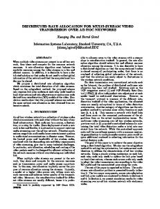
Fig. 3. Average number of iterations taken by Algorithm II until convergence
and Z5 is an appropriate normalization factor. IV. S IMULATION R ESULTS
In this section, we present simulation results for the two algorithms described in Section III. Incidence matrices of ' 1 dimensions {7 × 8, 8 × 10, 10 × 12, 15 × 18, 17 × 20, 18 × (l+1) (l) 2(l) gUi →Va (x) = Q(x; µVb →Ui , σVb →Ui ) exp(−βx2 ), 21, 20 × 24, 23 × 27, 25 × 30, 27 × 32, 30 × 36, 33 × 40, 35 × Z4 b"=a 42, 38 × 45, 40 × 48, 42 × 50, 47 × 56, 50 × 60} were simulated Vb ∈N(Ui ) for both algorithms. The matrices were generated so that their and Z4 is an appropriate normalization factor. 4. Belief calculation: Repeat Step 2 and Step 3 until the associated graphs do not contain cycles of length four for following (marginal) probability distribution converges to a smaller dimensions and of length up to 10 for larger dimensions using cycle removal techniques introduced in LDPC fixed distribution: code generation literature [4]. The degree of variable nodes (l+1) (l+1) 2(l+1) ), (7) was chosen to be three, and the degrees of constraint nodes fUi (x) = f (x; µUi , σUi were chosen randomly so that no degree-one constraint node where + * * + happens which can be trivially removed for reducing the graph. (l+1) 2(l+1) (l+1) = MV gUi (x) , µUi , σUi The probability density function resolution was set so that a ' total range of [−1, 3] is represented with 1024 points, instead 1 (l+1) (l) 2(l) Q(x; µVb →Ui , σVb →Ui ) exp(−βx2 ), of [−∞, ∞] for ease of computation. The algorithms were set gUi (x) = Z5 Vb ∈N(Ui ) to stop when there is no significant change in the distribution obtained in Step 4. Figure 10 illustrates an instance for the 3 Note that this is an approximation, and the real distribution is not necessarily Gaussian. evolution of the distribution of one variable node with an where
3 Authorized licensed use limited to: EPFL LAUSANNE. Downloaded on October 30, 2009 at 04:55 from IEEE Xplore. Restrictions apply.
Normalized error of Algorithm I on convergence to correct solution
0
−1
Normalized Error (E)
Normalized Error (E)
−1
10
−2
10
8 10
Fig. 4. solution
15
20
25
30 35 40 Number of Check Nodes
45
50
55
−2
10
10
60
Normalized error of Algorithm I on convergence to the correct
Normalized error of algorithm I on convergence
0
8 10
15
20
25
30 35 40 Number of Check Nodes
45
50
55
60
Fig. 7. Normalized error of Algorithm II on convergence to the correct solution
Normalized error of Algorithm II on convergence
0
10
10
−1
Normalized Error (E)
−1
Normalized Error (E)
10
−3
−3
10
Normalized error of Algorithm II on convergence to correct solution
0
10
10
10
−2
10
10
−2
10
−3
10
−3
10
10
Fig. 5.
15
20
25
30 35 40 Number of Check Nodes
45
50
55
60
8 10
Fig. 8.
Normalized error of Algorithm I on convergence
15
20
25
30 35 40 Number of Check Nodes
45
50
55
60
Normalized error of Algorithm II on convergence
Fraction of graphs where Algorithm II converged to correct solution 1
Fraction of graphs where Algorithm I converged to correct solution Fraction of graphs where correct solution was found
Fraction of graphs where correct solution was found
1 0.9 0.8 0.7 0.6 0.5 0.4 0.3 0.2
0.9 0.8 0.7 0.6 0.5 0.4 0.3 0.2 0.1
0.1 0 0
8 10
15
20
25
30 35 40 Number of Check Nodes
45
50
55
60
Fig. 6. Fraction of graphs where Algorithm I converged to the correct solution
Fig. 9. solution
8 10
15
20
25
30 35 40 Number of Check Nodes
45
50
55
60
Fraction of graphs where Algorithm II converged to the correct
4 Authorized licensed use limited to: EPFL LAUSANNE. Downloaded on October 30, 2009 at 04:55 from IEEE Xplore. Restrictions apply.
Initial Dist. After Iter. 1 Iter. 2 Iter. 3 Iter. 4 Iter. 5 Iter. 6 Final Iter. 14
8 7 6 Probability density
obtained by Algorithm 1. iii) the fluctuation in the fraction of “ill-conditioned” matrices along the dimension is smaller than that for Algorithm I. Therefore, we see that Algorithm II is more robust in a randomly chosen graph.
Evolving Distribution
9
5
V. D ISCUSSION In this section, we explain the relationship between the algorithms derived in Section III and the LP that defines the original problem. The LP (after a few simple manipulations) can be expressed as:
4 3 2
N $
min
{xUi }
1 0 −1
−0.8
−0.6
−0.4
−0.2
0
0.2
0.4
0.6
0.8
1
Fig. 10. An example of the evolution of probability distribution of a variable node
xUi
i=1
subject to (8) $ Constraint Va : xUk ≥ 1 for 1 ≤ a ≤ M, Uk ∈N(Va )
0 ≤ xUi ≤ 1 for 1 ≤ i ≤ N,
which can be written in terms of a an standard LP: 50 × 60 incidence matrix which converged in 14 iterations. We see from this figure that the peak of the distribution goes from zero to the region close to the solution, moves around the solution and finally converges to the solution. In Figures 2, 4, 6, and 5, we present, for Algorithm I, the average number of iterations until convergence, the normalized error between the true value and the algorithm’s output when the algorithm converges to the correct solution, the normalized error when the algorithm converges to a fixed point, and the fraction of graphs in the ensemble where the algorithm converges to the correct solution, respectively. The horizontal axis represents classes of matrices by the number of columns of matrices in the class. From Figure 2, we see that Algorithm I converges in around 15 iterations for most cases. The normalized error is defined by e(uBP ) =
&uBP − uLP &1 , &uLP &1
where uBP is the output of the proposed algorithm, and uLP is the solution of original formulation. The difference between the normalized error shown in Figure 4 and Figure 6 shows that there exists a collection of “ill-conditioned” matrices where Algorithm I fails to find the correct solution. Also, we see from Figure 5 that, for smaller dimension of incidence matrices, it is more likely that those “ill-conditioned” matrices happen. In Figures 3, 7, 8, and 9, the average number of iterations until convergence, the normalized error when the algorithm converges to the correct solution, the normalized error when the algorithm converges to a fixed point, and the fraction of graphs in the ensemble where the algorithm converges to the correct solution are respectively depicted for Algorithm II. There are several interesting observations about Algorithms II as follows: i) Algorithm II converges in 2 iterations in most cases, while the number of iterations for Algorithm I varies from 12 to 20. ii) the normalized error of (correct) solutions obtained by Algorithm II is smaller than those
min 1TN x x
subject to Ax ≥ 1M ,
(9)
where xUi denotes the rate value allocated to node Ui ∈ A1 , T x = [x1 , . . . , xUN ] , 1k is the k-dimensional all-one column vector, and A is the M × N incidence matrix where the entry at (i, j) is one if there is an edge between the node Vi ∈ A2 and the node Uj ∈ A1 ; otherwise the entry is zero. Since there is an explicit constraint that all xUi ’s be nonnegative, we can relax this constraint by changing the cost function to N $ i=1
(10)
|xUi |.
Also, let us define a function that is associated with each constraint Va ∈ A2 as follows: $ I xUk ≥ 1 , (11) Uk ∈N(Va )
where I(·) is the indicator function. In other words, the output value of this function is one if the variable nodes Ui in the N(Va ), otherwise zero. Using (10) and (11), the LP problem can be converted to the following unconstrained optimization problem: , M N $ ' $ I xUk ≥ 1 exp −β |xUk | , max {xUk }
a=1
Uk ∈N(Va )
k=1
(12)
where β is a nonnegative parameter that involves the convergence speed. The optimization problem like (12) can be solved using BP based message-passing techniques [9]. The messages defined in the Section III are updated according to the rules which are based on the probability of the
5 Authorized licensed use limited to: EPFL LAUSANNE. Downloaded on October 30, 2009 at 04:55 from IEEE Xplore. Restrictions apply.
event that each variable node takes a specific value at each time instant. Let XUi denote a (continuous) random variable associated with the rate value xUi . Here, there is an important underlying assumption: All messages on different edges in the network are independent. Thus, each type of messages has its (l) own probabilistic interpretation: The message MVa →Ui (x) can be interpreted as the probability density of XUi being forced to take a value x in order for the constraint Va to be satisfied. (l) Subsequently, the message mUi →Va (x) can be interpreted as the probability density of XUi being equal to x in order to satisfy all adjacent constraints when the constraint Va is absent from the network, i.e. a priori knowledge for the probability density of XUi provided by other adjacent constraint nodes. Thus, the belief calculated in the algorithms corresponds to the marginal probability density of each variable node. Also, the probability density of XUi being x in the event that the constraint Va is satisfied is straightforwardly calculated as: $ (l) fUi (x| XUk ≥ 1, XUk = uk ) Uk ∈N(Va )
1 = Z1
!
ui
I
$ k"=i
uk ≥ 1 − x
'
(l)
fUk (uk ) dui , (13)
k"=i Uk ∈N(Va )
(l)
where fUk (uk ) is a priori probability density of XUk , which (l) also corresponds to the message mUi →Va (x). Here, the distributions at variable nodes are assumed to be independent. Since (l) (13) corresponds to the definition of the message MVa →Ui (x), this message takes such form as (1). Moreover, the message (l) mUi →Va (x) is calculated by taking the product of probability density of XUi transferred from other constraint nodes in the sense of a prior knowledge. These update rules form Algorithm I. Although Algorithm I basically uses the probability densities as its messages, the algorithm can be simplified by a further assumption that the message distribution be Gaussian-like with a (minor) change in the objective function to: N $
x2Ui .
(14)
i=1
Then, the corresponding unconstrained optimization problem is given as , M N $ ' $ 2 max I xUk ≥ 1 exp −β xUk . (15) {xUk }
a=1
Uk ∈N(Va )
k=1
Note that the “local potential” term for XUi is a Gaussian function, and the constraint function basically involves a series of convolution operations followed by the calculation of Gaussian integral. Therefore, we can approximate messages transferred along the network to be Gaussian functions. Since, as mentioned in the previous section, the mean and the variance are sufficient statistics of Gaussian probability density under the approximation, the same procedure as Algorithm I can be performed by transferring only two parameters. Hence, Algorithm II is given as such.
VI. C OMPLEXITY ANALYSIS Here, we discuss the complexity of the proposed algorithms. Let L denote the number of points for the FFT operation to perform a convolution operation of two message distributions. For Algorithm I, a single edge processing at the constraint node update for a degree-dc constraint node involves dc − 2 convolutions and one integration, which are computationally equivalent to dc − 1 FFT’s and dc − 2 products of message distributions. Since there are mdc edges connected to constraint nodes, the complexity for constraint node updates is O(md2c L log L). Likewise, the complexity for variable node updates of degree dv is O(nd2v L). Therefore, the overall complexity of Algorithm I is O(nd2v L log L). For Algorithm II, the constraint node updates are simple because all operations can be replaced by addition operations. Since one integration and 2(dc − 2) additions are required for a single edge processing, the number of addition required for constraint node updates is O(mdc (dc + L)). If we use a lookup table for Q(x; µ, σ 2 ), the number of additions reduces to O(md2c ). Since variable node updates involve direct calculation of the first and second moment of message distributions, the overall number of multiplications and additions are O(nd2v L) and O(ndv L), respectively. Therefore, the overall complexity of Algorithm II is O(nd2v L). VII. C ONCLUSION In this work, we presented two distributed algorithms for the rate allocation problem over a coded multicast network. We provided simulation results which illustrates the convergence rate and correctness of these algorithms. R EFERENCES [1] M. Bayati, C. Borgs, J. Chayes, and R. Zecchina. Beliefpropagation for weighted b-matchings on arbitrary graphs and its relation to linear programs with integer solutions. Available at http://arxiv.org/abs/0709.1190, Feb. 2008. [2] D. Bertsekas and R. Gallager. Data networks. Prentice Hall, 1992. [3] T. Ho, M. M´ edard, R. Koetter, D. R. Karger, M. Effros, J. Shi, and B. Leong. A random linear network coding approach to multicast. IEEE Trans. on Info. Theory, 52(10):4413–4430, Oct. 2006. [4] X.-Y. Hu, E. Eleftheriou, and D. M. Arnold. Regular and irregular progressive edge-growth tanner graphs. IEEE Trans. Inform. Theory, 51(1):386–398, Jan. 2005. [5] J.M. Jaffe. Bottleneck flow control. IEEE Trans. on Comm., 29(7):954– 962, Jul. 1981. [6] M. Kim, M. M´ edard, V. Aggarwal, and U. M. O’Reilly. On the codinglink cost tradeoff in multicast network coding. Milit. Comm. Conf. (MILCOM), pages 1–7, Oct. 2007. [7] D. S. Lun, M. M´ edard, T. Ho, and R. Koetter. Network coding with a cost criterion. Int. Symp. on Info. Theory and its Appl. (ISITA), pages 1232–1237, Oct. 2004. [8] J. Mosely. Asynchronous Distributed Flow Control Algorithms. PhD thesis, Dept. of Elec. Eng. and Comp. Sci., MIT, Cambridge, Mass, Jun. 1984. [9] S. Sanghavi, D. Shah, and A. Willsky. Message-passing for maximum weight independent set. Available at http://arxiv.org/abs/0807.5091, Jul. 2008. [10] N. Sommer, M. Feder, and O. Shalvi. Low-density lattice codes. IEEE Trans. Inform. Theory, 54(4):1561–1585, Apr. 2008.
6 Authorized licensed use limited to: EPFL LAUSANNE. Downloaded on October 30, 2009 at 04:55 from IEEE Xplore. Restrictions apply.