2017 10th International Congress on Image and Signal Processing, BioMedical Engineering and Informatics( CISP-BMEI 2017)
Conditional Image Generation using Feature-Matching GAN Yuzhong Liu, Qiyang Zhao* and Cheng Jiang State Key Laboratory of Software Development Environment Department of Computer Science and Engineering, Beihang University Beijing 100191
[email protected]
Abstract—Generative Adversarial Net is a frontier method of generative models for images, audios and videos. In this paper, we focus on conditional image generation and introduce conditional Feature-Matching Generative Adversarial Net to generate images from category labels. By visualizing state-of-art discriminative conditional generative models, we find these networks do not gain clear semantic concepts. Thus we design the loss function in the light of metric learning to measure semantic distance. The proposed model is evaluated on several well-known datasets. It is shown to be of higher perceptual quality and better diversity then existing generative models. Keywords—Generative Adversarial Net; Image Generation; Deep Generative Model;
I. I NTRODUCTION Generative Adversarial Net (GAN) [5] is a framework of generative models, which is inspired by game theory. It is a two-player min-max game, where one plays the generator role and attempts to generate data samples from random noise, and another plays the discriminator attempts to discriminate synthetic samples and real ones. GAN does not have any assumptions about the data distribution. It learns the data distribution from the two-player game, and for the generation task it can generate more realistic samples than Variational Autoencoders (VAE) [7] and other method including PixelRNN [13]. The original GAN and its variants including Wasserstein GAN(WGAN) [2] try to learn the data distribution in an unsupervised way [14]. But in common application it usually needs more control to generate much better samples, this was called Condition GAN [11]. In Condition GAN, the generator attempts to generate from given labels together with random noise, and the discriminator attempts to discern the data sources as well as the data labels at the same time. In this procedure, the discriminator can give more effective gradients to the generator, and help it to generate higher quality samples. The discriminator is learned with label and data samples, thus it can be easily extended to semi-supervised learning [15]. In this paper, we investigate the theory of GAN through sample visualization analysis. We propose a novel way for semantic transfer in generation model, and we propose a Feature-Matching GAN model through metric learning in semantic representation. We first review the GAN theory in Section 2. In Sections 3, we present our Feature-Matching
978-1-5386-1936-0/17/$31 ©2017 IEEE
GAN extension of the GAN framework. In Section 4, we evaluate our framework on a variety of image generation tasks. II. BACKGROUNDS A. GAN The core idea of GAN is a two-player min-max game, which the players try to deceive each other. The goal of GAN is to train a generator network G which transforms vectors of noise z to data sample x. The training objective for G is defined by a discriminator D that is trained to distinguish samples from the generator distribution pgen (x) or real data distribution pdata (x). The generator network G aims to fool the discriminator to accept its outputs as real. The training procedure is training G and D by turns, finalizing to find a Nash equilibrium of the non-convex game. Unlike VAE and PixelRNN, GAN do not set any assumptions about the data distribution or have any model requirements. The GAN players are typically defined by neural networks, hence both player have sufficient large capacities. GAN are typically trained using gradient descent techniques that are designed to find a low value of a cost function. The total cost of GAN are formalized by V = Ex∼pdata (x) [log D(x)] + Ez∼pz (z) [log(1 − D(G(z)))] The total loss of GAN is defined to minimize the KL distance between data distribution and generated distribution. And given a fixed generator G, the optimal discriminator is given by Pdata (x) D∗ = Pdata (x) + PG (x) In GAN theory, Goodfellow [5] proved that given sufficient network capacities and an optimal discriminator D∗ , the generator G will recover the ture data distribution, so in this way pgen (x) = pdata (x). But in practical, the optimal discriminator is hard to find, so the better solution is to design effective evaluation criteria. A relant example is WGAN [2], which is proposed to employ Wasserstein distance instead of JensenShannon (JS) divergence to address the vanishing gradient problems.
c =1
real
real
real
fake
fake
fake
D
D
X real
X gen
X real
G Z (noise) GAN
c =2 ...
D X gen
G C (class )
real fake
X real
G
Z (noise)
C (class )
Conditional GAN
Z (noise)
AC-GAN
c =2 ...
D
D
X real
X gen
c =1
X gen
G C (class )
Z (noise)
FM-GAN(Our Model)
Fig. 1. GAN models. In these models, Z(noise) represents the random noise samples, Xreal and Xgen are real data samples and generated samples respectively. G is the generator and D is the discriminator. In the output of D, real and f ake are the data source labels, and c is the category label.
B. Conditional GAN The discriminator D is a discriminative network, which attempts to perform binary classification between data sources. A discriminator D will gain more accurate gradients if more classification information is given, as well as the generator G. Condition GAN is based on this idea and gives the data label to the generator and discriminator both. Data labels in generation and discrimination steps transform the original GAN model to a conditional way. The objective of Conditional GAN can thus be formalized by V = Ex∼pdata (x) [log D(x|y)]+Ez∼pz (z) [log(1−D(G(z|y)))] In the formula, the generator attempts to generate data from both random noise and data lable, and the discriminator attempts to discriminate data source given both samples and labels. Thus Condition GAN learns a conditional generation model, and the input label controls the generated samples. Though Conditional GAN enhanced the stablity, but fails to learn the semantic difference between the data samples. ACGAN [12] extend this idea, the discriminator D attempts to classify the data source and data label at the same time, thus the label gridients can strengthen the discriminator learning ability. The objective of a AC-GAN can be formalized by
layer should be also similar. Feature maps of the middle layers of the neural network can be expressed as input features. In image retrieval and object detection, raw images are usually replaced with inner feature maps as model input. In GAN the feature matching (FM) procedure [15] are the matching loss between real data samples and generated samples in feature maps space, this loss are defined in statistics thus will prevent the generator G from overfitting of the discriminator D. As shown in the following equation, common F Mloss is the Euclidean distance for generated samples and the real samples at layer l of D F Mloss = ∥Ex∼pdata Dl (x) − Ez∼pz (z) Dl (G(z))∥22 F Mloss is defined the distance between two distributions, it enhanced the model stablity and reduce the missing mode samples. However low variance problem is usually caused by the statistics loss. III. C ONDITIONAL F EATURE M ATCHING GAN
Conditional GAN extends the theory of GAN by adding the label information, but in semantic visualization experiments we find the conditional GAN model can hardly learn meaningful semantic representations. In this section, we first introduce semantic visualizing methods for GAN, then propose a new LS = E[log P (S = real|Xreal )]+E[log P (S = f ake|Xf ake )] feature matching generation model from the perspective of metric learning. LC = E[log P (C = c|Xreal )] + E[log P (C = c|Xf ake )] In the formula, L is the data source output, and the L is A. Semantic Visualization Experiment S
C
the data label output. In AC-GAN, the discriminator D tries to maximize LS + LC , generator G tries to minimize LC − LS . C. Feature Matching Losses Neural networks are layers stacked with non-linear mapping, thus if the input is similar, the feature maps of the middle
The understanding of how deep neural networks work, especially the model decision theory is important. As we all know, activations and loss gradients in each layer contain some semantic informations. In previous work, Condition GAN and Improved GAN use conditional label and feature matching method make generation more stable, and improve
(a) ResNet Visualization
the distances and extend it to semantic feature matching: 1) Feature Matching: the original feature matching distance is measured between real samples and generated samples in statistics, however label informations are neglected. Thus generated samples are of low variances and high bias. In Fig. 2, the gradients on AC-GAN indicate the network do not learn useful features. In our work, we alter the distance to every single label, the altered feature loss on layer l is defined as F eatureloss = ∥Ex∼pdata f l (x|y) − Ez∼pz (z) f l (G(z)|y)∥22
(b) AC-GAN Visualization Fig. 2. Image-specific class saliency map and classification map. From left to right are respectively input image, saliency map and classification map. Saliency map shows gradient in every pixel, and in classification map show probability in every two pixel and in the map warmer color indicates higher probability. a) results of ResNet, with the label true tower. b) results of ACGAN, with the true label male.
the accuracy semi-supervised classification. But almost all existing conditional GAN model can hardly generate large scale samples in high quality, potential because both generator and discriminator hardly learn much semantic representation of the label. Here we choose Saliency Map and Classification Map to visualize the discriminator network activations [16] [20]. Saliency map is defined as the label gradient on input image piexls, the given label on the image is expected to have strong activations on the pixels, and the correspanding gradients should be much helpful for image segmentation and object detection. Classification map is defined as the probability heat map of the label in image pixels. We choose two networks, ResNet [6] and the discriminator of AC-GAN. ResNet is an well-defined network for image classification [3]. The visualization experiment is desireable for compare the semantic difference between networks. To the best of our knowledge, this is the first work about visualizing GAN models. The visualization results are showed in Fig. 2. We can see ResNet learns pretty good semantic representation of the image label. In contrast, the discriminator of AC-GAN barely learns semantic representation well, and the gradients of the label is nearly randomly placed. Nevertheless, the generator networks in GAN can hardly draw efficient support from both saliency maps in Fig. 2. It means the current network can not used as discriminators to provide strong semantic information. B. Metric Learning for GAN The semantic gradient indicates the weak discrimination boundary in generative model, causing under-fitting in GAN. For sake of this, several distances are proposed to minimize the difference between data sources [15] [21]. Here we review
Compared with original F Mloss , F eatureloss is more accurate in semantic matching between data samples. And the proposed loss is based on label aware thus can gererate high variance samples. 2) Style Matching: style loss is style distance between images [4]. It measures the texture difference, and usually used in image transfer. As we all know, image style is location free, thus it is better to measure the similarity between two images. In image transfer, the style loss is original defined as the similarity between the two vectors. In our work, we extend style loss to every single labe, the proposed style loss is defined as ∑ Styleloss = f l (x|y)f l (G(z)|y) Combining the definition about content and feature above, the discriminator D learns the semantic difference between the real data and generate samples. The above distance give more accurate gradient on semantic manner, and do not increase time complexity. Algorithm 1 Minibatch gradient descent training of FM-GAN for number of training iterations do • Sample minibatch of real data {x(1) , .., x(m) } and the correspanding data label {c(1) , .., c(m) } from dataset. • Sample minibatch of noise sample {z (1) , .., z (m) } from noise distribution pg (z). Sample minibatch of generate samples from generator G given by noise z and lable c. • Calculate the F eatureloss and Styleloss between two data sources. Calculate the data source loss LS and LC . • Update the discriminator D by ascending the gradient: 1 ∑ (−LS − LC + F eatureloss + Styleloss ) m i=1 m
∇θD
• Sample minibatch of noise sample {z (1) , .., z (m) } from noise distribution pg (z). Sample minibatch of generate samples from generator G given by noise z and lable c. • Calculate the F eatureloss and Styleloss between two data sources. Calculate the data source loss LS and LC . • Update the generator G by ascending the gradient: 1 ∑ (LS − LC − F eatureloss − Styleloss ) ∇θG m i=1 m
end for
Real data
Improved GAN
CGAN
AC-GAN
Our model
Fig. 3. MNIST samples from different GAN models. Each row is conditioned on one label. Fig. 4. FM-GAN generation on CIFAR-10 dataset, each row conditioned on one label.
C. Feature-Matching GAN Using the semantic metric loss defined in metric manner, we get our Feature-Matching GAN (FM-GAN). The proposed model is shown in Fig. 1 together with original GAN, Conditional GAN and AC-GAN for comparison. Compared with existing GAN models, our FM-GAN can learn more accurate gradient on data source and data label, thus can generate more realistic sample by using data label. To our knowledge, the proposed model is the first GAN model using metric learning. The objective function of our model can be formalized by
A. MNIST [9] The MNIST dataset contains 60,000 labeled images of digits, and each image is 28×28 grey style. We compare generated samples of different GAN models in Fig. 3. As the generated examples show, our model are more diversified and realistic. Samples are fair random draws, not cherry-picked. And all generation models are trained with same epoch. B. CIFAR-10 [8]
LD = −LS − LC + F eatureloss + Styleloss
CIFAR-10 is a well studied dataset of 32×32 natural images, which contains 60,000 labeled images in 10 classes. Compared with MNIST, CIFAR-10 is hard to generate visual samples, and it is usually for image diversity comparison. We first conduct generation task on this dataset, as shown in Fig. 4. The proposed model learns semantic representation on the dataset, this is claimed that the semantic metric loss is effective. Then we performe a series of capacity experiments† to demonstrate that our proposed model can generate more diversity examples. To do quantitative comparison, all generation model are trained with same epoch. The result is presented in Table. I, our model outperform the existed generation models in different all capacity state. This shows that our model can generate diverse samples.
LG = LS − LC − F eatureloss − Styleloss It is claimed the generator G will recover the ture data distribution in state of optimal discriminator D, thus the gradients are more accurate and the generated samples are more realistic. The procedure is formally presented in Algorithm 1. Unlike AC-GAN, our model learns the semantic representation in both generator and discriminator, which can give direct gradient on label, and prevents the generator overfitting from the discriminator. IV. E XPERIMENT
C. CelebA [10] In this section, we experimentally analyze our proposed method in generation tasks. Images is high dimensions spaese data, thus it is hard evaluate the similarity between two distributions. Evaluating GAN and the generated samples is still an open problem [19]. The original work uses Gaussian Parzen windows for evaluation, but it is known perform bad in high dimensions. Hence we choose Inception score [15], a well defined metric for evaluation in the fellowing experiments.
CelebA is a large-scale face attributes dataset, and each face with 40 attribute annotations. In this task we use it for face †
Inception Score is defined by exp(Ex [DKL (p(y|x)||p(y))]), where x is the input image and p(y|X) is the conditional class output in the pretrained Inception network on CIFAR-10. Inception Score measure the distance between the conditional output and the dataset labele distribution. We use the Inception-v3 [17] version to compute the score, which supplied in https://github.com/openai/improved-gan/
TABLE I I NCEPTION SCORES ON CIFAR-10 Model GAN [5] WGAN [2] Improved GAN [15] Conditional GAN [11] AC-GAN [12] FM-GAN Real Data
1K 5.34 4.79 3.98 5.75 5.65 5.79 8.80
Image numbers 5K 10K 25K 5.79 5.92 6.06 5.67 5.78 5.83 4.15 4.28 4.34 6.19 6.47 6.44 5.87 6.17 6.30 5.91 6.37 6.75 10.69 10.99 11.15
ACKNOWLEDGMENT 50K 6.07 5.88 4.36 6.47 6.35 6.79 11.95
Fig. 5. FM-GAN generation on CelebA dataset. Samples in each rows are of the same attributes. The first and the second rows are Male and Female, the third and the fourth rows are Male with Smile and Female with Smile, the fifth and the sixth rows are Male with Black hair and Female with Brown hair.
generation experiments. Each face contains multiple attributes, and these image attributes can be used to control the sample generation. We use these attributes to make a conditional sample generation, the results are showed in Fig 5. V. C ONCLUSION Generative adversarial networks are the frontier method of generative models. In this paper we focus on conditional generation model, and we find the weak discrimination boundary in generative model via visualization experiments. This work presents one solution to solve the problem. We introduce a novel conditional generation model, which is constructed by semantic representation losses in metric learning manner. The proposed model can measures the semantic distance between different data samples. The generation tasks demonstrate our model can produce higher quality and better diversity than the existing methods in qualitative and quantitative evaluation. However the current GAN experiments are commonly on small scale datasets, how to promote its to large scale datasets is still a challenge.
We like to thank the developers of Tensorflow [1] and Theano [18] for the great software used to implement our idea. R EFERENCES [1] Mart´ın Abadi, Ashish Agarwal, Paul Barham, Eugene Brevdo, Zhifeng Chen, Craig Citro, Greg S Corrado, Andy Davis, Jeffrey Dean, Matthieu Devin, et al. Tensorflow: Large-scale machine learning on heterogeneous distributed systems. arXiv preprint arXiv:1603.04467, 2016. [2] Martin Arjovsky, Soumith Chintala, and L´eon Bottou. Wasserstein gan. arXiv preprint arXiv:1701.07875, 2017. [3] Jia Deng, Wei Dong, Richard Socher, Li-Jia Li, Kai Li, and Li FeiFei. Imagenet: A large-scale hierarchical image database. In Computer Vision and Pattern Recognition, 2009. CVPR 2009. IEEE Conference on, pages 248–255. IEEE, 2009. [4] Leon A Gatys, Alexander S Ecker, and Matthias Bethge. Image style transfer using convolutional neural networks. In Proceedings of the IEEE Conference on Computer Vision and Pattern Recognition, pages 2414–2423, 2016. [5] Ian Goodfellow, Jean Pouget-Abadie, Mehdi Mirza, Bing Xu, David Warde-Farley, Sherjil Ozair, Aaron Courville, and Yoshua Bengio. Generative adversarial nets. In Advances in neural information processing systems, pages 2672–2680, 2014. [6] Kaiming He, Xiangyu Zhang, Shaoqing Ren, and Jian Sun. Deep residual learning for image recognition. In Proceedings of the IEEE conference on computer vision and pattern recognition, pages 770–778, 2016. [7] Diederik P Kingma and Max Welling. Auto-encoding variational bayes. arXiv preprint arXiv:1312.6114, 2013. [8] Alex Krizhevsky and Geoffrey Hinton. Learning multiple layers of features from tiny images. 2009. [9] Yann LeCun. The mnist database of handwritten digits. http://yann. lecun. com/exdb/mnist/, 1998. [10] Ziwei Liu, Ping Luo, Xiaogang Wang, and Xiaoou Tang. Deep learning face attributes in the wild. In Proceedings of the IEEE International Conference on Computer Vision, pages 3730–3738, 2015. [11] Mehdi Mirza and Simon Osindero. Conditional generative adversarial nets. arXiv preprint arXiv:1411.1784, 2014. [12] Augustus Odena, Christopher Olah, and Jonathon Shlens. Conditional image synthesis with auxiliary classifier gans. arXiv preprint arXiv:1610.09585, 2016. [13] Aaron van den Oord, Nal Kalchbrenner, and Koray Kavukcuoglu. Pixel recurrent neural networks. arXiv preprint arXiv:1601.06759, 2016. [14] Alec Radford, Luke Metz, and Soumith Chintala. Unsupervised representation learning with deep convolutional generative adversarial networks. arXiv preprint arXiv:1511.06434, 2015. [15] Tim Salimans, Ian Goodfellow, Wojciech Zaremba, Vicki Cheung, Alec Radford, and Xi Chen. Improved techniques for training gans. In Advances in Neural Information Processing Systems, pages 2234–2242, 2016. [16] Karen Simonyan, Andrea Vedaldi, and Andrew Zisserman. Deep inside convolutional networks: Visualising image classification models and saliency maps. arXiv preprint arXiv:1312.6034, 2013. [17] Christian Szegedy, Vincent Vanhoucke, Sergey Ioffe, Jon Shlens, and Zbigniew Wojna. Rethinking the inception architecture for computer vision. In Proceedings of the IEEE Conference on Computer Vision and Pattern Recognition, pages 2818–2826, 2016. [18] Theano Development Team. Theano: A Python framework for fast computation of mathematical expressions. arXiv e-prints, abs/1605.02688, May 2016. [19] Lucas Theis, A¨aron van den Oord, and Matthias Bethge. A note on the evaluation of generative models. arXiv preprint arXiv:1511.01844, 2015. [20] Matthew D Zeiler and Rob Fergus. Visualizing and understanding convolutional networks. In European conference on computer vision, pages 818–833. Springer, 2014. [21] Zhiming Zhou, Shu Rong, Han Cai, Weinan Zhang, Yong Yu, and Jun Wang. Generative adversarial nets with labeled data by activation maximization. arXiv preprint arXiv:1703.02000, 2017.