Cross-view image synthesis using geometry-guided conditional GANs

Cross-view image synthesis using geometry-guided conditional GANs Krishna Regmi∗∗, Ali Borji Center for Research in Computer Vision (CRCV), University of Central Florida, Orlando, FL, USA

arXiv:1808.05469v1 [cs.CV] 14 Aug 2018

ABSTRACT

We address the problem of generating images across two drastically different views, namely ground (street) and aerial (overhead) views. Image synthesis by itself is a very challenging computer vision task and is even more so when generation is conditioned on an image in another view. Due the difference in viewpoints, there is small overlapping field of view and little common content between these two views. Here, we try to preserve the pixel information between the views so that the generated image is a realistic representation of cross view input image. For this, we propose to use homography as a guide to map the images between the views based on the common field of view to preserve the details in the input image. We then use generative adversarial networks to inpaint the missing regions in the transformed image and add realism to it. Our exhaustive evaluation and model comparison demonstrate that utilizing geometry constraints adds fine details to the generated images and can be a better approach for cross view image synthesis than purely pixel based synthesis methods.

1. Introduction Novel view synthesis is a long-standing problem in computer vision. Earlier works in this area synthesize views of single objects or natural scenes with small variation in viewing angle. For generating views of single objects in a uniform background or scenes, the task regards learning a mapping or transformation across views. With a small camera movement, there is a high degree of overlap in field of views resulting in images with high content overlap. The generative models can learn to copy large parts of the image content from the input to the output and perform the synthesis task satisfactorily. Despite this, view synthesis task is very challenging due to presence of multiple objects in the scene. The network needs to learn the object relations and occlusions in the scene. Generating cross-view natural scenes conditioned on images from drastically different views (e.g., generating top-view from street view scene) is very painstaking. This is mainly because there is very little overlap between the corresponding field of views. Thus, simply copying and pasting pixels from one view to another would not be a solution. Rather, it is needed to learn the object classes present in the input view and to understand the correspondences in the target view with appropriate object relations and transformations (i.e., geometric reasoning). In this work, we address the problem of synthesizing groundlevel images from overhead imagery and vice versa using conditional Generative Adversarial Networks [Mirza and Osindero (2014)]. Also, when possible, we guide the generative networks by feeding homography transformed images as inputs to improve the synthesized results. Basically, conditional GANs try to generate new images from conditioning variables as input.

∗∗ Corresponding

author: e-mail: [email protected] (Krishna Regmi) This work extends our CVPR 2018 paper [Regmi and Borji (2018)]

The conditioning variables could be other images, text descriptions, class labels, etc. Our first approach exploits the success of the first GANbased image-to-image translation network put forward by Isola et al. (2017) as a general purpose architecture on multiple image translation tasks. This work translates images of objects or scenes which are represented by RGB images, gradient fields, edge maps, aerial images, sketches, etc across these representations. Thus, it essentially operates on different representations of images in a single view. We use this architecture as a starting point (base model) in our task and obtain encouraging results. The limitation of this approach to our problem, however, is that the images to be transformed to are very different as they come from two drastically different views, have small fields of view overlap, and objects in the images might be occluded. As a result, learning to map the pixels between the views is difficult as the corresponding pixels in two views may represent different object classes. To address this challenge, here we propose to use the semantic segmentation maps of target view images to regularize the training process. This helps the network learn the semantic class of the pixels in the target view and guides the network to generate the target pixels. The next approach we take to solve the cross-view image synthesis task is to exploit the geometric relation between the views to guide the synthesis. For this, we first compute the homography transformation matrix between the views and then project the aerial images to street-view perspective. By doing so, we obtain an intermediate image that looks very close to the target view image but not as realistic and with some missing regions. Now, our problem reduces to preserving the scene layout and details while filling in the missing regions and adding realism to the transformed image. For this, we use cGAN architectures described in previous approach. We also use different cGANs that work specifically for inpainting and realism tasks to preserve the pixel information from the homography transformed image in a controlled manner. To summarize, we propose the following methods. We start with the simple image-to-image translation network of Isola

2 et al. (2017) as a baseline (here called Pix2pix). We then propose two new cGAN architectures that generate images as well as segmentation maps in the target view. Augmenting semantic segmentation generation to the architectures helps improve the quality of generated images. The first architecture, called X-Fork, is a slight modification of the baseline, forking at the penultimate block to generate two outputs, target view image and segmentation map. The second architecture, called X-Seq, has a sequence of two baseline networks connected. The target view image generated by the first network is fed to the second to generate its corresponding segmentation map. Once trained, both architectures are able to generate better images than the baseline that generates only the target view images. This implies that learning to generate segmentation map along with the image indeed improves the quality of generated images. We also use homography to transform the aerial image to ground view and feed the transformed image to these networks to further improve the results. Finally, we propose a method to preserve details from the homography transformed image in a controlled setting to generate the street view images. It constitutes two subtasks: a) generating missing regions by inpainting, and b) adding realism by using GAN to preserves details visible in aerial view into the street view image. We call this approach H-Regions. Throughout the paper, H in a method’s name indicates that the input is the homography transformed image. 2. Related Work 2.1. Relating Aerial and Ground-level Images Zhai et al. (2017) explored the relationship between the cross-view images by learning to predict the semantic layout of the ground image from its corresponding aerial image. They used the predicted layout to synthesize ground-level panorama. Prior works relating the aerial and ground imageries have addressed problems such as cross-view co-localization [Lin et al. (2013); Vo and Hays (2016)], ground-to-aerial geo-localization [Lin et al. (2015); MH and Lee (2018)] and geo-tagging the cross-view images [Workman et al. (2015)]. Cross-view relations have also been studied between egocentric (first person) and exocentric (surveillance or third-person) domains for different purposes. Human re-identification by matching viewers in top-view and egocentric cameras have been tackled by establishing the correspondences between the views in Ardeshir and Borji (2016). Soran et al. (2014) utilize the information from one egocentric camera and multiple exocentric cameras to solve the action recognition task. 2.2. Learning View Transformations Existing works on viewpoint transformation have been conducted to synthesize novel views of the same objects [Dosovitskiy et al. (2017); Tatarchenko et al. (2016); Zhou et al. (2016)]. Zhou et al. (2016) proposed models that learn to copy the pixel information from the input view and utilize them to preserve the identity and structure of the objects to generate new views. Tatarchenko et al. (2016) trained an encode-decoder network to obtain 3D models of cars and chairs which they later used to generate different views of an unseen car or chair. Dosovitskiy

et al. (2017) learned generative models by training on 3D renderings of cars, chairs and tables and synthesized intermediate views and objects by interpolating between views and models. 2.3. GAN and cGAN Goodfellow et al. (2014) are the pioneers of Generative Adversarial Networks that are very successful at generating sharp and unblurred images, much better compared to existing methods such as Restricted Boltzmann Machines [Hinton et al. (2006); Smolensky (1986)] or deep Boltzmann Machines [Salakhutdinov and Hinton (2009)]. Conditional GANs synthesize images conditioned on different parameters during both training and testing. Examples include conditioning on labels of MNIST to generate digits by Mirza and Osindero (2014), on image representations to translate an image between different representations by Isola et al. (2017), and generating panoramic ground-level scenes from aerial images of the same location by Zhai et al. (2017). Reed et al. (2016) synthesize images conditioned on detailed textual descriptions of the objects in the scene, and Zhang et al. (2017) improved on that by using a two-stage Stacked GAN. 2.4. Cross-Domain Transformations using GANs Kim et al. (2017) utilized the GAN networks to learn the relation between images in two different domains such that these learned relations can be transferred between the domains. Similar work by Zhu et al. (2017) learned mappings between unpaired images using cycle-consistency loss. They assume that a mapping from one domain to the other and back to the first should generate the original image. Both works exploited large unpaired datasets to learn the relation between domains and formulated the mapping task between images in different domains as a generation problem. Zhu et al. (2017) compare their generation task with previous works on paired datasets by Isola et al. (2017). They conclude that the result with paired images is the upper-bound for their unpaired examples. 2.5. Geometry-guided Synthesis Song et al. (2017) propose geometry-guided adversarial networks to synthesize identity-preserving facial expressions. The facial geometry is used as a controlled input to guide the network to synthesize facial images with desired expressions. Similar work by Kossaifi et al. (2017) improves the visual quality of synthesized images by enforcing a mechanism to control the shapes of the objects. They map the generator’s output to a mean shape and implicitly enforce the geometry of the objects and also add skip connections to transfer priors to the generated objects. 2.6. Image Inpainting Pathak et al. (2016) generated missing parts of images using networks trained jointly with adversarial and reconstruction losses and produced sharp and coherent images. Yeh et al. (2017) tackle the problem of image inpainting by searching for the encoding of the corrupted image that is closest to another image in the latent space and passing it through the generator to reconstruct the image. The closeness is defined based on the weighted context loss of the corrupted image, and a prior loss

3 that penalizes unrealistic images. Yang et al. (2017) propose a multi-scale patch synthesis approach for high-resolution image inpainting by jointly optimizing on image content and texture constraint. 3. Background on GANs Th Generative Adversarial Network (GAN) proposed by Goodfellow et al. (2014) consists of two adversarial networks: a generator and a discriminator that are trained simultaneously based on the min-max game theory. The generator G is optimized to map a d-dimensional noise vector (usually d=100) to an image (i.e., synthesizing) that is close to the true data distribution. The discriminator D, on the other hand, is optimized to accurately distinguish between the synthesized images coming from the generator and the real images coming from the true data distribution. The objective function of such a network is

min max L (G, D) = E x ∼ pdata (x) [logD(x)]+ G D GAN Ez ∼ pz (z) [log(1 − D(G(z)))],

+E x0 ,c ∼ pdata (x0 ,c) [log(1 − D(x0 , c))],

(2)

where x0 = G(z, c) is the generated image. In addition to the GAN loss, previous works [e.g., Isola et al. (2017); Zhu et al. (2017); Pathak et al. (2016)] have tried to minimize the L1 or L2 distances between real and generated image pairs. This step aids the generator to synthesize images very similar to the ground truth. Minimizing the L1 distance generates less blurred images than minimizing the L2 distance. That is, using the L1 distance increases image sharpness in generation tasks. Therefore, we use the L1 distance in our method. The expression to minimize the L1 distance is

min L (G) = E 0 ∼ 0 x,x pdata (x,x0 ) [|| x − x ||1 ], G L1

+E Ia ,Ig0 ∼ pdata (Ia ,Ig0 ) [log(1 − D(Ig0 , Ia ))],

min L (G) = E 0 ∼ 0 Ig ,Ig pdata (Ig ,Ig0 ) [|| Ig − Ig ||1 ], G L1

(5)

where Ig0 = G(Ia ). The objective function for an image-to-image translation network is the sum of conditional GAN loss in Eqn. (4) and L1 loss in Eqn. (5), as represented in Eqn. (6):

Lnetwork = LcGAN (G, D) + λLL1 (G),

(6)

where, λ is the balancing factor between the losses. 4. Framework In this section, we discuss the baseline methods and the proposed architectures for the task of cross-view image synthesis.

(1)

where x is real data sampled from data distribution pdata and z is a d-dimensional noise vector sampled from a Gaussian distribution pz . Conditional GANs synthesize images looking into some auxiliary variable which may be labels [Mirza and Osindero (2014)], text embeddings [Zhang et al. (2017); Reed et al. (2016)] or images [Isola et al. (2017); Zhu et al. (2017); Kim et al. (2017)]. In conditional GANs, both the discriminator and the generator networks receive the conditioning variable represented by c in Eqn. (2). The generator uses this additional information during image synthesis while the discriminator makes its decision by looking at the pair of conditioning variable and the image it receives. Real pair input to the discriminator consists of true image from distribution and its corresponding label while the fake pair consists of the synthesized image and the label. For conditional GAN, the objective function is

min max L (G, D) = E x,c ∼ pdata (x,c) [logD(x, c)] G D cGAN

are represented as in Eqns. (4) and (5), respectively. For ground to aerial synthesis, the roles of Ia and Ig are reversed. min max L (G, D) = E Ig ,Ia ∼ pdata (Ig ,Ia ) [logD(Ig , Ia )] G D cGAN (4)

(3)

The objective function for such conditional GAN network is the sum of Eqns. (2) and (3). Considering the synthesis of the ground level imagery (Ig ) from aerial image (Ia ), the conditional GAN loss and L1 loss

4.1. Baselines The naive way to approach this task is to consider it as an image to image translation problem. We run the experiments in the following settings as our baselines. 4.1.1. Cross-view Image-to-Image Translation (X-Pix2pix) For this, we use an encoder-decoder network that takes in an image in first view as input and learns to generate the image in the other view as output. 4.1.2. Cross-view Image-to-Image Translation with Stacked Outputs (X-SO) The network takes an image in first view as input and generates target view image and the segmentation map stacked together as a 6-channel image; first 3 channels for image and the next three channels for its segmentation mask. 4.2. Proposed Methods 4.2.1. Crossview Fork (X-Fork) Our first architecture, known as the Crossview Fork, is shown in Figure 1a. The generator network is forked to synthesize images as well as segmentation maps. The fork-generator architecture is shown in Figure 2. The first six blocks of decoder share the weights. This is because the image and segmentation map contain a lot of shared features. The number of kernels used in each layer (block) of the generator are shown below the blocks. The inherent idea behind this architecture is multi-task learning by the generator network. When the generator is enforced to learn the semantic class of the pixels together with the image synthesis, this helps to improve the image synthesis task. The generated segmentation map serves as an auxiliary output. The objective function for this network is shown in Eqn. 7. LX−Fork = LcGAN (G, D) + λLL1 (G(Ig , Ig0 )) + λLL1 (G(S g , S g0 ))

(7)

Note that the L1 loss is minimized for images as well as segmentation maps whereas the adversarial loss is optimized for images only. This is because we only care about pixel accuracy for segmentation maps.

4 Ia

Sg’

Generator Network G Ia Ig

Convolution + lReLU (CL)

Ig’ Ia

&

Convolution + BN + lReLU (CBL)

P(real) ~ [0,1]

Discriminator Network D

&

Upconvolution + BN + ReLU (UBR) Upconvolution + BN + Dropout + ReLU(UBDR)

512 512

(a) X-Fork architecture.

Street view Image 512 512

512256

128 64

Ig’

Generator Network G1

Ia

Generator Network G2

Ia Ia Ig

Discriminator Network D1

Sg’ Aerial Image

Ig’

64

512 512 512 512 256 512 128 512 512 512

Street view Segmentation 512 512

256 128 64

Sg Ig’

P(real) ~ [0,1]

Discriminator Network D2

Fig. 2: Generator of X-Fork architecture in Figure 1a. BN means batch-normalization layer. The first six blocks of decoder share weights, forking at the penultimate block. The number of channels in each convolution layer are shown below each blocks.

P(real) ~ [0,1]

(b) X-Seq architecture.

Fig. 1: Our proposed network architectures. a) X-Fork: Similar to baseline architecture except that G forks to synthesize image and segmentation map in target view, and b) X-Seq: a sequence of two cGANs, G1 synthesizes target view image that is used by G2 for segmentation map synthesis in corresponding view. In both architectures, Ia and Ig are real images in aerial and ground views, respectively. S g is the ground-truth segmentation map in street-view obtained using pretrained RefineNet Lin et al. (2017). Ig0 and S g0 are synthesized image and segmentation map in ground view.

4.2.2. Crossview Sequential (X-Seq) Our second architecture uses a sequence of two cGAN networks as shown in Figure 1b. The first network performs crossview image synthesis and the generated image is fed to the second network as a conditioning input to synthesize its corresponding segmentation map. This two-stage end-to-end learning of image and segmentation map synthesis produces improved image quality compared to the network without second stage. The joint objective function for X-Seq architecture is shown in Eqn. 8 below.

LX−S eq = Lnetwork (G1 , D1 ) + Lnetwork (G2 , D2 )

(8)

4.2.3. Cross-view Pix2pix with Homography (H-Pix2pix) Another approach that we take here is to feed the homography transformed image as an input to the translation network. Our hypothesis is that the majority of the scene from the first view is transformed into the second perspective using the homography and this should ease the synthesis task. The large missing regions in the transformed images are mostly related to sky and buildings. 4.2.4. Cross-view Stacked Outputs with Homography (H-SO) The network takes the homography transformed image as input and generates target view image and the segmentation map stacked together as a 6-channel image; first 3 channels for image and the next three channels for its segmentation map. 4.2.5. Cross-view Fork with Homography (H-Fork) Here, we use the homography transformed image Iah as input to the network architecture proposed in subsection 4.2.1.

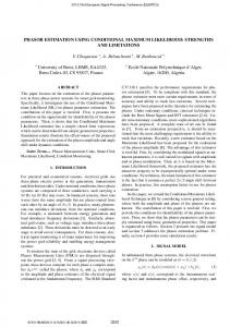
The hypothesis behind this idea is that the use of transformed images as input should ease the cross-view synthesis task compared to synthesizing by feeding the aerial images Ia directly. 4.2.6. Crossview Sequence with Homography (H-Seq) In this setup, we feed the homography transformed image Iah rather than the original input image Ia as input to the X-Seq network of subsection 4.2.2. 4.2.7. Crossview Regions with Homography (H-Regions) In this method, we attempt to preserve the structural details visible in the aerial view images and guide the network to transfer those details to the synthesized ground view images. For this, we use the homography transformed image as input to our method and solve the synthesis task in following subtasks: Subtask I: The homography transformed image (Iah in Figure 3) has a large portion of missing region (R1 ) in the image. Our first task is to fill in the missing region in the transformed images. We use an encoder-decoder network that takes Iah as input and generates only the upper half of the image (Ig0 ). Subtask II: The street-view images are recorded by a camera mounted on a car’s dashboard. Therefore, all the street-view images contain a part of the car’s hood around the lower central region (R2 ) in them which can be seen in image Ig in Figure 3. The homography transformed image Iah also has a car around that region which has been transformed from the aerial view of the car but it does not realistically represent a car in streetview. To address this, we mask a probable car-region and train a small network dedicated to learn mapping of the car region. This helps generate a realistic car region in ground view images (See region R2 in image Ig0 ). Once we have images generated from the first two tasks, we copy them to their respective spatial locations in homography transformed image Iah creating a street-view image Ig0 and preserving the pixels of remaining regions. Copying pixels in this manner helps us preserve the structural information that has been transformed using homography. The problem with this approach is that images do not look realistic at region boundaries. So, we further train another network to add realism to this image. Subtask III: GANs are successful at generating images that look very realistic to human eyes. Here, we train a conditional

5 R1 R2 Ia Iah Ig’ Ig Fig. 3: For an aerial image, Ia shown in the left, we first transform it into street-view perspective using homography (Iah) as shown in second image from left. The transformed image needs inpainting in upper box region (R1 ) and requires further transforming of car region (R2 ). These two regions are generated and the region in between is copied from homography transformed image Iah to obtain Ig’. We further train Ig0 to smooth the region boundaries and add realism to the image. Ig is the corresponding ground truth image.

GAN architecture on Ig0 . For this, we first define bands around the region boundaries as shown in Figure 3. We formulate the loss function to preserve (by copying) the pixel information outside the bands to the output image while at the same time adding realism to the whole image. This step helps a lot to improve the visual quality of the synthesized image. We now define our loss functions for the subtasks. For subtask one, we use conditional GAN network to inpaint missing regions in Iah by optimizing the network on adversarial and L1 losses for the missing regions only. For subtask two, we only consider region R2 by masking out the remaining regions in input and output images and optimizing for adversarial and L1 losses for car region only. Once we have results from the above two subtasks, we compute I0g as shown in Eqn. 9. Ig0 = IInpaint M1 + Icar M2 + Iah (M - M1 - M2 )

(9)

Here, IInpaint is the image generated from the inpainting network of subtask one. Icar is the car image generated in subtask two. M1 and M2 are 3-channel binary masks for regions R1 and R2 , M being the 3-channel all ones image. Ig0 is fed to the realism network to generate the final image in the target view. is the element-wise product. 5. Experimental Setting 5.1. Datasets For the experiments in this work, we use three datasets described in the following. Dayton. This cross-view image dataset is provided by Vo and Hays (2016). It consists of more than 1M pairs of street-view and overhead view images collected from 11 different US cities. We select 76,048 image pairs from Dayton images and create a train/test split of 55,000/21,048 pairs. We call it Dayton Dataset. The images in the original dataset have resolution of 354×354. We resize them to 256×256. We use this dataset for experiments in both aerial to ground a2g and ground to aerial g2a directions. CVUSA. We recruit this dataset [Workman et al. (2015)] for direct comparison of our work with Zhai et al. (2017). It consists of 35,532/8,884 train/test split of image pairs. Following Zhai et al. (2017), the aerial images are center-cropped to 224 × 224 and then resized to 256 × 256. We only generate a single camera-angle image rather than the panorama. To do so,

Fig. 4: Original image pairs from training set (left), images with segmentation masks from pre-trained RefineNet (Lin et al. (2017)) overlaid on original images (middle) and images with segmentation masks generated by X-Fork network overlaid on original images (right).

we take the first quarter of the ground level images as well as segmentations from the dataset and resize them to 256 × 256 in our experiments. SVA. The Surround Vehicle Awareness (SVA) dataset [Palazzi et al. (2017)] is a synthetic dataset collected from Grand Theft Auto V (GTAV) video game. The game camera is toggled between frontal and bird’s eye view to simultaneously capture images in the two views at each game time step. We use the train/test split as provided in the dataset. The original dataset has 100 sets of training set images and 50 sets of test set images. The consecutive frames in each set are very similar to each other, so we use every tenth frame to remove redundancy in the dataset. Finally, we have a training set of 46,030 image pairs and a test set of 22,254 image pairs. The images are resized to 256 × 256 for experiments in this work. Sample images from SVA dataset are shown in the leftmost and rightmost columns of Figure 7. We use this dataset for experiments in aerial to ground a2g direction only. Note that, homography related experiments are performed on this dataset only. The proposed Fork and Sequence networks learn to generate the target view images and segmentation maps conditioned on source view image or their homography transformed image. Training procedure requires the images as well as their semantic segmentation maps. The CVUSA dataset has annotated segmentation maps for ground view images, but for SVA and Dayton datasets such information is not available. To compensate, we use one of the leading semantic segmentation methods, known as the RefineNet [Lin et al. (2017)]. This network is pre-trained on outdoor scenes of the Cityscapes dataset [Cordts et al. (2016)] and is used to generate the segmentation maps that are utilized as ground truth maps. These semantic maps have pixel labels from 20 classes (e.g., road, sidewalk, building, vegetation, sky, void, etc). Figure 4 shows image pairs from the Dayton dataset and their segmentation masks overlaid in both views. As can be seen, the segmentation mask (label) generation process is not perfect since it is unable to segment parts of buildings, roads, cars, etcetera in images. 5.2. Implementation Details We use homography as a preprocessing step to transform the visual features from aerial images to ground perspective. Since the locations of aerial and ground view camera are fixed in the SVA dataset, first we randomly pick a pair of images from the dataset. We then manually select four points in the aerial image and find their corresponding locations in the ground-view image and use them to compute the homography matrix that transforms the aerial image to ground view and vice versa. Surprisingly, this method works well and avoids expensive compu-

6 tations for homography estimation usually done for each pair of images separately by computing SIFT features of the images and then finding the keypoints in the images. We also tried computing the SIFT features and then finding keypoints in two images and transforming images based on those points. This method could not find the corresponding points in two views, most likely because of very large perspective variation between the views. We use the conditional GAN architecture very similar to Isola et al. (2017) as the base architecture. The generator is an encoder-decoder network with blocks of Convolution, Batch Normalization [Ioffe and Szegedy (2015)] and activation layers. Leaky ReLU with a slope of 0.2 is used as the activation function in the encoder, whereas the decoder has ReLU activation except for its final layer where Tanh is used. The first three blocks of the decoder have a Dropout layer in between Batch normalization and activation layer, with dropout rate of 50%. The discriminator is taken as it is from the Isola et al. (2017). For the experiments on the SVA dataset, we removed two blocks of CBL and UBDL from the generator architecture, primarily to save training time. We observed that removal of these blocks did not have much impact on the quality of synthesized images. The convolutional kernels used in the networks are 4×4 in size with a stride of 2. The upconvolution in the decoder is Torch [Collobert et al. (2011)] implementation of S patialFullConvolution, and upsamples the input by 2. The convolutional operation downsamples the images by 2. No pooling operation is used in the networks. The λ used in the objective function for different networks is the balancing factor between the GAN loss and the L1 loss. Its value is fixed at 100 for Fork and Seq models. For realism task in the H-Regions method, we use two lambdas, λ1 =5 for adversarial loss and λ2 =2 for pixel-wise loss. Following the idea to smooth the labels by Szegedy et al. (2016) and demonstration of its effectiveness by Salimans et al. (2016), we use one-sided label smoothing to stabilize the training process, replacing 1 by 0.9 for real labels. During the training, we utilized different data augmentation methods such as random jitter and horizontal flipping of images. The network is trained end-to-end with weights initialized using a random Gaussian distribution with zero mean and 0.02 standard deviation. Our methods are implemented in Torch [Collobert et al. (2011)]. Code is publicly available 2 . We train the networks for 100 epochs on low resolution and 35 epochs on high resolution images of Dayton dataset and for 20 epochs on SVA dataset. Experiments are conducted on CVUSA dataset for comparison with the work of Zhai et al. (2017). Following their setup, we train our architectures for 30 epochs using the Adam optimizer and moment parameters β1 = 0.5 and β2 = 0.999. We observed that the training for XSO method on low resolution of Dayton dataset and CVUSA dataset was very unstable; so the qualitative and quantitative results are not very good for them. For H-Regions, we conduct experiments as follows. For subtask I, we train the network for 20 epochs. For subtask II, we train another network for one

2 https://github.com/kregmi/cross-view-image-synthesis

epoch only since the network needs to learn the mapping of the car and to preserve its color from source view to the target view. Eventually, we train a final realism network for 5 epochs (subtask III). 6. Evaluation and Model Comparison We have conducted experiments in a2g (aerial-to-ground) and g2a (ground-to-aerial) directions on Dayton dataset and a2g direction only on CVUSA dataset and SVA dataset. We consider image resolutions of 64×64 and 256×256 on Dayton dataset while for experiments on CVUSA and SVA datasets, 256×256 resolution images are used. 6.1. Evaluation measures It is not straightforward to evaluate the quality of synthesized images [Borji (2018)]. In fact, evaluation of GAN methods continues to be an open problem [Theis et al. (2016)]. Here we use four quantitative measures and a qualitative measure to evaluate our methods. 6.1.1. Qualitative measures For subjective evaluation of different methods, we run a user study on the images synthesized using these methods. We show an aerial image along with the corresponding images in ground view synthesized using seven different methods to 10 users. We specifically ask each user to select the most realistic image that also contains the most visual details from the aerial view image. 6.1.2. Quantitative measures Inception Score: A common quantitative measure used in GAN evaluation is the Inception Score by Salimans et al. (2016). The core idea behind the inception score is to assess how diverse the generated samples are within a class while being meaningfully representative of the class at the same time. One major criticism regarding Inception score is that the CNN trained on ImageNet objects may not be adequate for other scene datasets (our case). To address this, here we use the AlexNet model [Krizhevsky et al. (2017)] trained on Places dataset [Zhou et al. (2017)] with 365 categories to compute the inception score. The Places dataset has images similar to those in our datasets. We observe that the confidence scores predicted by the pretrained model on our datasets are dispersed between classes for many samples and not all the categories are represented by the images. Therefore, we compute inception scores on Top-1 and Top-5 classes, where ”Top-k” means that top k predictions for each image are unchanged while the remaining predictions are P smoothed by an epsilon equal to (1 - (top-k predictions))/(n-k classes). Accuracy: In addition to inception score, we compute the topk prediction accuracy between real and generated images. We use the same pre-trained Alexnet model to obtain annotations for real images and class predictions for generated images. We compute top-1 and top-5 accuracies. For each setting, accuracies are computed in two ways: 1) considering all images, and 2) considering real images whose top-1 (highest) prediction is greater than 0.5. Below each accuracy heading, the first column

7 considers all images whereas the second column computes accuracies the second way. KL(model k data): We compute the KL divergence between the model generated images and the real data distribution for quantitative analysis of our work, similar to some generative works [Che et al. (2016); Nguyen et al. (2017)]. We again use the same pre-trained Alexnet described earlier. The lower KL score implies that the generated samples are closer to the real data distribution. SSIM, PSNR and Sharpness Difference: We employ three measures from the image quality assessment literature to evaluate our models, similar to Mathieu et al. (2015); Ledig et al. (2017); Shi et al. (2016); Park et al. (2017)). StructuralSimilarity (SSIM) measures the similarity between the images based on their luminance, contrast and structural aspects. SSIM value ranges between -1 and +1. Peak Signal-to-Noise Ratio (PSNR) measures the peak signal-to-noise ratio between two images to assess the quality of a transformed (generated) image compared to its original version. Sharpness difference (SD) measures the loss of sharpness during image generation. For each of these score, the higher the the better. Please refer to Regmi and Borji (2018) for details on how to compute these scores. 6.2. Model Comparison We conduct the qualitative and quantitative evaluation on 3 datasets. We report homography results on SVA dataset only. This is because the aerial view image for SVA dataset contains high overlap with the field of view of street-view image and thus application of homoraphy to preserve the details from aerial image seemed valid for this dataset compared to the other two. We conduct the user studies to compare the images synthesized using different methods as well as illustrate qualitative results in Figures 5, 6 and 7 and conduct an in-depth quantitative evaluation on test images of the datasets. 6.2.1. Qualitative Comparison Dayton dataset. For 64×64 resolution experiments, the networks are modified by removing the last two blocks of CBL from discriminator and encoder, and the first two blocks of UBDR from decoder of the generator. We run experiments on all three methods. Qualitative results are depicted in Figure 5 (left). The results affirm that the networks have learned to transfer the image representations across the views. Generated ground level images clearly show details about road, trees, sky, clouds, and pedestrian lanes. Trees, grass, road, house roofs are well rendered in the synthesized aerial images. For 256×256 resolution synthesis, we conduct experiments on all three architectures and illustrate the qualitative results in Figure 5 (right). We observe that the images generated in high resolution contain more details of objects in both views and are less granulated than those in low resolution. Houses, trees, pedestrian lanes, and roads look more natural. CVUSA dataset. Test results on the CVUSA dataset show that images generated by proposed methods are visually better compared to Zhai et al. (2017) and Isola et al. (2017). The images generated by our proposed methods are more successful in

Table 1: % of user preferences over images synthesized by different methods (over 100 images from the SVA dataset). X-Pix2pix X-Fork X-Seq H-Pix2pix H-Fork H-Seq H-Reg. 4

7.8

16.8

12.6

14.2

18.2

26.4

transforming the pixel classes and thus generating correct class objects in target view compared to the baselines. SVA dataset. The qualitative results on the SVA dataset for aerial to street-view synthesis is shown in Figure 7. The proposed methods are capable at generating roads, car-hood, markers on road, sky and other details in the images. We observe that the images generated by the proposed H-Regions method contain more details around the central regions. This is due to enforcing the network to preserve those details from the aerial images. User Study. We conducted the perceptual test over 100 test images on 10 subjects to compare the images synthesized by different methods on the SVA dataset. The results are presented in Table 1. The most preferred method is H-Regions, closely contested by H-Seq and X-Seq methods. The results illustrate the following: a) The use of homography transformed input drastically outperforms corresponding experiments with untransformed aerial image as input, and b) Users preferred the images synthesized using H-Regions because of the method’s ability to preserve the pixel information onto the target view. 6.2.2. Quantitative Comparison We report the quantitative results on three datasets next. Dayton dataset. The quantitative scores over different measures are provided in Tables 2, 3, 4 and 5 under the columns Dayton (64 x 64) and Dayton (256 x 256) for low and high resolution synthesis. Inception Score: The scores for X-Fork generated images are closest to that of real data distribution for Dayton dataset in low resolution in both directions and also in high resolution in a2g direction. The X-Seq method works best for g2a synthesis in high resolution for Dayton dataset. Inception scores on top-k classes follow a similar pattern as in all classes (except for Top1 class on low resolution and Top-5 class on high resolution in g2a direction over Dayton dataset). Accuracy: Results are shown in Table 3. We observe that the X-Fork method works better at low resolution whereas X-Seq is better at high resolution synthesis in both directions. KL(model k data): The scores are provided in Table 4. As it can be seen, our proposed methods generate much better results than the baselines. X-Fork generates images very similar to real distribution in all experiments except on the high resolution a2g experiment where X-Seq is slightly better than X-Fork. SSIM, PSNR, and SD: The scores are reported in Table 5. The X-Seq model works the best in a2g direction while X-Fork outperforms the rest in the g2a direction. CVUSA dataset. The quantitative evaluation is shown in Tables 2, 3, 4 and 5 under the column CVUSA. Inception Score: The X-Seq method works best for CVUSA dataset in terms of inception score. Accuracy: Results are shown in Table 3. Images generated with X-Fork method obtain the best accuracy closely followed by X-Seq method.

8 a2g synthesis Pix2pix X-SO X-Fork X-Seq

g2a a2g

g2a synthesis Pix2pix X-SO X-Fork X-Seq

a2g synthesis Pix2pix X-SO X-Fork X-Seq

g2a a2g

g2a synthesis Pix2pix X-SO X-Fork X-Seq

Fig. 5: Example images generated by different methods in low (64 × 64) resolution (left) and high (256 × 256) resolution (right) in a2g and g2a directions on the Dayton dataset. Table 2: Inception Scores of models over Dayton and CVUSA datasets. Dir. 

a2g

g2a

Methods

Zhai et al. (2017) X-Pix2pix X-SO X-Fork X-Seq Real Data X-Pix2pix X-SO X-Fork X-Seq Real Data

a2g synthesis

Zhai et al

Dayton (64 × 64) all Top-1 Top-5 classes class classes – – – 1.8029 1.5014 1.9300 1.8577 1.4975 2.0301 1.9600 1.5908 2.0348 1.8503 1.4850 1.9623 2.2096 1.6961 2.3008 1.7970 1.3029 1.6101 1.4798 1.2163 1.5042 1.8557 1.3162 1.6521 1.7854 1.3189 1.6219 2.1408 1.4302 1.8606 Pix2pix

X-SO

X-Fork

X-Seq

Fig. 6: Qualitative results of our methods and baselines on CVUSA dataset in a2g direction. First two columns show true image pairs, next four columns show images generated by Zhai et al. (2017), X-Pix2pix [Isola et al. (2017)], X-SO, X-Fork and X-Seq methods respectively.

KL(model k data): The scores are provided in Table 4. As it can be seen, our proposed methods generate much better results than the baseline. X-Fork generates images very similar to real distribution and X-Seq very close to it. SSIM, PSNR, and SD: Images generated using X-Fork are better than other methods in terms of SSIM, PSNR and SD. We find that X-Fork improves over Zhai et al. by 5.03% in SSIM, 8.93% in PSNR, and 12.35% in SD. SVA dataset. The quantitative evaluation on SVA dataset is illustrated in Table 6. Inception Score: H-Regions generates images that have the inception score closest to that of real data. Accuracy: H-Seq method performs best in terms of accuracy. KL(model k data): Images synthesized using X-Seq method

Dayton (256 × 256) all Top-1 Top-5 classes class classes – – – 2.8515 1.9342 2.9083 2.9459 2.0963 2.9980 3.0720 2.2402 3.0932 2.7384 2.1304 2.7674 3.7090 2.5590 3.7900 3.5676 2.0325 2.8141 3.3397 2.0232 3.3485 3.1342 1.8656 2.5599 3.5849 2.0489 2.8414 3.8979 2.3146 3.1682

all classes 1.8434 3.2771 1.7575 3.4432 3.8151 4.9971 – – – – –

CVUSA Top-1 class 1.5171 2.2219 1.4145 2.5447 2.6738 3.4122 – – – – –

Top-5 classes 1.8666 3.4312 1.7791 3.5567 4.0077 5.1150 – – – – –

have the closest distribution to the ground truth distribution among all the methods. SSIM, PSNR, and SD: X-Seq achieves the highest numbers in terms of SSIM and PSNR whereas H-Regions has the best SD. Also, H-Pix2pix already performs very good compared to XPix2pix because homography simplified the learning task by transforming the image to the target view. H- methods outperform their X- counterparts for most of the evaluation metrics. Because there is no consensus in evaluation of GANs, we had to use several scores. Theis et al. (2016) show that these scores often do not agree with each other and this was observed in our evaluations as well. Nonetheless, we find that the proposed methods are consistently superior to the baselines in terms of quantitative and qualitative evaluations.

7. Discussion and Conclusion We explored image generation using conditional GANs between two drastically different views. Generating semantic segmentations together with images in target view helps the networks learn better images compared to the baselines. Using homography to guide the cross-view synthesis allows preserving the overlapping regions between the views. Extensive qualitative and quantitative evaluations testify the effectiveness of our methods. The challenging nature of the problem leaves room for further improvements. Potential application of this work can be in the direction of cross-view image geo-localization.

9 Aerial

Homography X-Pix2pix

X-SO

X-Fork

X-Seq

H-Pix2pix

H-SO

H-Fork

H-Seq

H-Regions

GT

Fig. 7: Example images generated by different methods in a2g direction for SVA dataset. Table 3: Accuracies: Top-1 and Top-5 on Dayton and CVUSA datasets. Dir. 

a2g

g2a

Methods

Zhai et al. (2017) X-Pix2pix X-SO X-Fork X-Seq X-Pix2pix X-SO X-Fork X-Seq

Dayton (64 × 64) Top-1 Top-5 Accuracy (%) Accuracy (%) – – – – 7.90 15.33 27.61 39.07 4.68 7.49 16.72 24.96 16.63 34.73 46.35 70.01 4.83 5.56 19.55 24.96 1.65 2.24 7.49 12.68 0.10 0.00 0.98 0.28 4.00 16.41 15.42 35.82 1.55 2.99 6.27 8.96

Dayton (256 × 256) Top-1 Top-5 Accuracy (%) Accuracy (%) – – – – 6.8 9.15 23.55 27.00 27.56 41.15 57.96 73.20 30.00 48.68 61.57 78.84 30.16 49.85 62.59 80.70 10.23 16.02 30.90 40.49 8.52 12.57 27.35 32.76 10.54 15.29 30.76 37.32 12.30 19.62 35.95 45.94

Table 4: KL Divergence between model and data distributions on

CVUSA Top-1 Top-5 Accuracy (%) Accuracy (%) 13.97 14.03 42.09 52.29 7.33 9.25 25.81 32.67 0.29 0.21 6.14 9.08 20.58 31.24 50.51 63.66 15.98 24.14 42.91 54.41 – – – – – – – – – – – – – – – –

gence 39, 692–705. URL: http://lmb.informatik.uni-freiburg.

Dayton and CVUSA datasets. de/Publications/2017/DTB17. Goodfellow, I., Pouget-Abadie, J., Mirza, M., Xu, B., Warde-Farley, D., Ozair, Dir. Method Dayton(64×64) Dayton(256×256) CVUSA S., Courville, A., Bengio, Y., 2014. Generative adversarial nets, in: AdZhai et al. (2017) – – 27.43 ± 1.63 vances in neural information processing systems, pp. 2672–2680. X-Pix2pix 6.29 ± 0.8 38.26 ± 1.88 59.81 ± 2.12 Hinton, G.E., Osindero, S., Teh, Y.W., 2006. A fast learning algorithm for a2g X-SO 4.99 ± 0.71 7.20 ± 1.37 414.25 ± 2.37 deep belief nets. Neural Comput. 18, 1527–1554. URL: http://dx. X-Fork 3.42 ± 0.72 6.00 ± 1.28 11.71 ± 1.55 doi.org/10.1162/neco.2006.18.7.1527, doi:10.1162/neco.2006. X-Seq 6.22 ± 0.87 5.93 ± 1.32 15.52 ± 1.73 18.7.1527. X-Pix2pix 6.39 ± 0.90 7.88 ± 1.24 – Ioffe, S., Szegedy, C., 2015. Batch normalization: Accelerating deep network X-SO 16.45 ± 0.96 9.15 ± 1.22 – training by reducing internal covariate shift, in: Proceedings of the 32Nd g2a X-Fork 4.45 ± 0.84 6.92 ± 1.15 – International Conference on International Conference on Machine LearnX-Seq 7.20 ± 0.92 7.07 ± 1.19 –

References Ardeshir, S., Borji, A., 2016. Ego2top: Matching viewers in egocentric and top-view videos, in: Computer Vision - ECCV 2016 - 14th European Conference, Amsterdam, The Netherlands, October 11-14, 2016, Proceedings, Part V, pp. 253–268. URL: https://doi.org/10.1007/ 978-3-319-46454-1_16, doi:10.1007/978-3-319-46454-1_16. Borji, A., 2018. Pros and cons of gan evaluation measures. arXiv preprint arXiv:1802.03446 . Che, T., Li, Y., Jacob, A.P., Bengio, Y., Li, W., 2016. Mode regularized generative adversarial networks. arXiv e-prints abs/1612.02136. URL: https://arxiv.org/abs/1612.02136. Collobert, R., Kavukcuoglu, K., Farabet, C., 2011. Torch7: A matlab-like environment for machine learning, in: BigLearn, NIPS Workshop. Cordts, M., Omran, M., Ramos, S., Rehfeld, T., Enzweiler, M., Benenson, R., Franke, U., Roth, S., Schiele, B., 2016. The cityscapes dataset for semantic urban scene understanding, in: Proc. of the IEEE Conference on Computer Vision and Pattern Recognition (CVPR). Dosovitskiy, A., Springenberg, J.T., Tatarchenko, M., Brox, T., 2017. Learning to generate chairs, tables and cars with convolutional networks. IEEE Transactions on Pattern Analysis and Machine Intelli-

ing - Volume 37, JMLR.org. pp. 448–456. URL: http://dl.acm.org/ citation.cfm?id=3045118.3045167. Isola, P., Zhu, J.Y., Zhou, T., Efros, A.A., 2017. Image-to-image translation with conditional adversarial networks. CVPR . Kim, T., Cha, M., Kim, H., Lee, J.K., Kim, J., 2017. Learning to discover cross-domain relations with generative adversarial networks, in: Precup, D., Teh, Y.W. (Eds.), Proceedings of the 34th International Conference on Machine Learning, PMLR, International Convention Centre, Sydney, Australia. pp. 1857–1865. URL: http://proceedings.mlr.press/v70/kim17a. html. Kossaifi, J., Tran, L., Panagakis, Y., Pantic, M., 2017. Gagan: Geometry-aware generative adverserial networks. arXiv preprint arXiv:1712.00684 . Krizhevsky, A., Sutskever, I., Hinton, G.E., 2017. Imagenet classification with deep convolutional neural networks. Commun. ACM 60, 84–90. URL: http://doi.acm.org/10.1145/3065386, doi:10.1145/3065386. Ledig, C., Theis, L., Huszar, F., Caballero, J., Cunningham, A., Acosta, A., Aitken, A.P., Tejani, A., Totz, J., Wang, Z., Shi, W., 2017. Photo-realistic single image super-resolution using a generative adversarial network, in: 2017 IEEE Conference on Computer Vision and Pattern Recognition, CVPR 2017, Honolulu, HI, USA, July 21-26, 2017, pp. 105–114. URL: https: //doi.org/10.1109/CVPR.2017.19, doi:10.1109/CVPR.2017.19. Lin, G., Milan, A., Shen, C., Reid, I., 2017. RefineNet: Multi-path refinement networks for high-resolution semantic segmentation, in: CVPR. Lin, T., Cui, Y., Belongie, S.J., Hays, J., 2015. Learning deep representations

10 Table 5: SSIM, PSNR and Sharpness Difference between real data and samples generated using different methods on Dayton and CVUSA datasets. Dir. Methods Dayton (64 × 64) Dayton (256 ×256) CVUSA 

SSIM

PSNR

SD

SSIM

PSNR

SD

SSIM

PSNR

SD

a2g

Zhai et al. (2017) X-Pix2pix X-SO X-Fork X-Seq

– 0.4808 0.4960 0.4921 0.5171

– 19.4919 19.7442 19.6273 20.1049

– 16.4489 16.6670 16.4928 16.6836

– 0.4180 0.4772 0.4963 0.5031

– 17.6291 19.6203 19.8928 20.2803

– 19.2821 19.2939 19.4533 19.5258

0.4147 0.3923 0.3451 0.4356 0.4231

17.4886 17.6578 17.6201 19.0509 18.8067

16.6184 18.5239 16.9919 18.6706 18.4378

g2a

X-Pix2pix X-SO X-Fork X-Seq

0.3675 0.3254 0.3682 0.3663

20.5135 16.5433 20.6933 20.4239

14.7813 16.2329 14.7984 14.7657

0.2693 0.2620 0.2763 0.2725

20.2177 19.9827 20.5978 20.2925

16.9477 16.8748 16.9962 16.9285

– – – –

– – – –

– – – –

Table 6: Quantitative evaluation of samples generated using different methods on SVA Dataset in a2g direction. Methods

X-Pix2pix

X-SO

X-Fork

X-Seq

H-Pix2pix

H-SO

H-Fork

H-Seq

H-Regions

*Inception Score, all *Inception Score, Top-1 *Inception Score, Top-5

2.0131 1.7221 2.2370

2.4951 1.8940 2.6634

2.1888 1.9776 2.3664

2.2232 1.9842 2.4344

2.1906 1.9507 2.4069

2.3202 1.9410 2.7340

2.3202 1.9525 2.3918

2.2394 1.9892 2.4385

2.6328 2.0732 2.8347

Accuracy (Top-1, all) Accuracy (Top-1, 0.5) Accuracy (Top-5, all) Accuracy (Top-5, 0.5)

8.5961 30.3288 9.0260 29.9102

7.5146 30.9507 10.3905 38.9822

17.3794 53.4725 23.8315 63.5045

19.5056 57.1010 25.8807 65.3005

18.0706 54.8068 23.4400 62.3072

5.2444 26.4697 5.2544 31.9527

18.0182 51.0756 26.6746 62.8166

20.7391 57.5378 28.5517 67.4649

15.4803 48.0767 21.8225 56.8994

KL(model || data)

19.5553

12.0906

4.1925

3.7585

4.2894

12.8761

4.7246

4.4260

6.0638

SSIM PSNR SD

0.3206 0.4552 0.4235 0.4638 0.4327 0.4457 0.424 0.4249 17.9944 21.5312 21.24 22.3411 21.686 21.7709 21.6327 21.4770 17.0254 17.5285 16.9371 17.4138 16.9468 17.3876 16.8653 17.5616 *Inception Score for real (ground truth) data is 3.0347, 2.3886 and 3.3446 for all, top-1 and top-5 setups respectively.

for ground-to-aerial geolocalization, in: IEEE Conference on Computer Vision and Pattern Recognition, CVPR 2015, Boston, MA, USA, June 7-12, 2015, pp. 5007–5015. URL: https://doi.org/10.1109/CVPR.2015. 7299135, doi:10.1109/CVPR.2015.7299135. Lin, T.Y., Belongie, S., Hays, J., 2013. Cross-view image geolocalization, in: The IEEE Conference on Computer Vision and Pattern Recognition (CVPR). Mathieu, M., Couprie, C., LeCun, Y., 2015. Deep multi-scale video prediction beyond mean square error. CoRR abs/1511.05440. URL: http://dblp. uni-trier.de/db/journals/corr/corr1511.html#MathieuCL15. MH, S.H.M.F.R., Lee, N.G.H., 2018. Cvm-net: Cross-view matching network for image-based ground-to-aerial geo-localization, in: Proceedings of the IEEE Conference on Computer Vision and Pattern Recognition, pp. 7258– 7267. Mirza, M., Osindero, S., 2014. Conditional generative adversarial nets. CoRR abs/1411.1784. URL: http://arxiv.org/abs/1411.1784. Nguyen, T.D., Le, T., Vu, H., Phung, D., 2017. Dual discriminator generative adversarial nets, in: Advances in Neural Information Processing Systems 29 (NIPS), p. accepted. Palazzi, A., Borghi, G., Abati, D., Calderara, S., Cucchiara, R., 2017. Learning to map vehicles into bird’s eye view, in: Battiato, S., Gallo, G., Schettini, R., Stanco, F. (Eds.), Image Analysis and Processing - ICIAP 2017, Springer International Publishing, Cham. pp. 233–243. Park, E., Yang, J., Yumer, E., Ceylan, D., Berg, A.C., 2017. Transformationgrounded image generation network for novel 3d view synthesis. CoRR abs/1703.02921. URL: http://arxiv.org/abs/1703.02921. Pathak, D., Krahenbuhl, P., Donahue, J., Darrell, T., Efros, A.A., 2016. Context encoders: Feature learning by inpainting, in: Proceedings of the IEEE Conference on Computer Vision and Pattern Recognition, pp. 2536–2544. Reed, S., Akata, Z., Yan, X., Logeswaran, L., Schiele, B., Lee, H., 2016. Generative adversarial text to image synthesis, in: Balcan, M.F., Weinberger, K.Q. (Eds.), Proceedings of The 33rd International Conference on Machine Learning, PMLR, New York, New York, USA. pp. 1060–1069. URL: http://proceedings.mlr.press/v48/reed16.html. Regmi, K., Borji, A., 2018. Cross-view image synthesis using conditional gans, in: The IEEE Conference on Computer Vision and Pattern Recognition (CVPR). Salakhutdinov, R., Hinton, G.E., 2009. Deep boltzmann machines., in: International Conference on Artificial Intelligence and Statistics (AISTATS), p. 3.

0.4044 20.9848 17.6858

Salimans, T., Goodfellow, I.J., Zaremba, W., Cheung, V., Radford, A., Chen, X., 2016. Improved techniques for training gans, in: Advances in Neural Information Processing Systems 29: Annual Conference on Neural Information Processing Systems 2016, December 5-10, 2016, Barcelona, Spain, pp. 2226–2234. URL: http://papers.nips.cc/ paper/6125-improved-techniques-for-training-gans. Shi, W., Caballero, J., Huszar, F., Totz, J., Aitken, A.P., Bishop, R., Rueckert, D., Wang, Z., 2016. Real-time single image and video super-resolution using an efficient sub-pixel convolutional neural network, in: 2016 IEEE Conference on Computer Vision and Pattern Recognition, CVPR 2016, Las Vegas, NV, USA, June 27-30, 2016, pp. 1874–1883. URL: https: //doi.org/10.1109/CVPR.2016.207, doi:10.1109/CVPR.2016.207. Smolensky, P., 1986. Parallel distributed processing: Explorations in the microstructure of cognition, vol. 1, MIT Press, Cambridge, MA, USA. chapter Information Processing in Dynamical Systems: Foundations of Harmony Theory, pp. 194–281. URL: http://dl.acm.org/citation.cfm?id= 104279.104290. Song, L., Lu, Z., He, R., Sun, Z., Tan, T., 2017. Geometry guided adversarial facial expression synthesis . Soran, B., Farhadi, A., Shapiro, L.G., 2014. Action recognition in the presence of one egocentric and multiple static cameras, in: Cremers, D., Reid, I.D., Saito, H., Yang, M. (Eds.), Computer Vision - ACCV 2014 - 12th Asian Conference on Computer Vision, Singapore, Singapore, November 1-5, 2014, Revised Selected Papers, Part V, Springer. pp. 178–193. URL: https://doi.org/10.1007/978-3-319-16814-2_12, doi:10.1007/ 978-3-319-16814-2_12. Szegedy, C., Vanhoucke, V., Ioffe, S., Shlens, J., Wojna, Z., 2016. Rethinking the inception architecture for computer vision, in: 2016 IEEE Conference on Computer Vision and Pattern Recognition, CVPR 2016, Las Vegas, NV, USA, June 27-30, 2016, pp. 2818–2826. URL: https://doi.org/10. 1109/CVPR.2016.308, doi:10.1109/CVPR.2016.308. Tatarchenko, M., Dosovitskiy, A., Brox, T., 2016. Multi-view 3d models from single images with a convolutional network, in: Leibe, B., Matas, J., Sebe, N., Welling, M. (Eds.), Computer Vision – ECCV 2016, Springer International Publishing, Cham. pp. 322–337. Theis, L., van den Oord, A., Bethge, M., 2016. A note on the evaluation of generative models, in: International Conference on Learning Representations. URL: http://arxiv.org/abs/1511.01844. Vo, N.N., Hays, J., 2016. Localizing and Orienting Street Views Using

11 Overhead Imagery. Springer International Publishing, Cham. pp. 494– 509. URL: http://dx.doi.org/10.1007/978-3-319-46448-0_30, doi:10.1007/978-3-319-46448-0_30. Workman, S., Souvenir, R., Jacobs, N., 2015. Wide-area image geolocalization with aerial reference imagery, in: IEEE International Conference on Computer Vision (ICCV). Yang, C., Lu, X., Lin, Z., Shechtman, E., Wang, O., Li, H., 2017. Highresolution image inpainting using multi-scale neural patch synthesis, in: The IEEE Conference on Computer Vision and Pattern Recognition (CVPR), p. 3. Yeh, R.A., Chen, C., Lim, T.Y., Schwing, A.G., Hasegawa-Johnson, M., Do, M.N., 2017. Semantic image inpainting with deep generative models, in: Proceedings of the IEEE Conference on Computer Vision and Pattern Recognition, pp. 5485–5493. Zhai, M., Bessinger, Z., Workman, S., Jacobs, N., 2017. Predicting groundlevel scene layout from aerial imagery, in: IEEE Conference on Computer Vision and Pattern Recognition (CVPR). Zhang, H., Xu, T., Li, H., Zhang, S., Wang, X., Huang, X., Metaxas, D., 2017. Stackgan: Text to photo-realistic image synthesis with stacked generative adversarial networks, in: ICCV. Zhou, B., Lapedriza, A., Khosla, A., Oliva, A., Torralba, A., 2017. Places: A 10 million image database for scene recognition. IEEE Transactions on Pattern Analysis and Machine Intelligence . Zhou, T., Tulsiani, S., Sun, W., Malik, J., Efros, A.A., 2016. View synthesis by appearance flow, in: Leibe, B., Matas, J., Sebe, N., Welling, M. (Eds.), Computer Vision – ECCV 2016, Springer International Publishing, Cham. pp. 286–301. Zhu, J.Y., Park, T., Isola, P., Efros, A.A., 2017. Unpaired image-to-image translation using cycle-consistent adversarial networkss, in: Computer Vision (ICCV), 2017 IEEE International Conference on.