Artificial Neural Networks - Advances in Computational Intelligence and Learning. Bruges (Belgium), 23-25 April 2008, d-side publi., ISBN 2-930307-08-0.
ESANN'2008 proceedings, European Symposium on Artificial Neural Networks - Advances in Computational Intelligence and Learning Bruges (Belgium), 23-25 April 2008, d-side publi., ISBN 2-930307-08-0.
Conditional Prediction of Time Series Using Spiral Recurrent Neural Network Huaien Gao1,2 , Rudolf Sollacher2 1- University of Munich, Germany 2- Siemens AG, Corporate Technology, Germany Abstract. Frequently, sequences of state transitions are triggered by specific signals. Learning these triggered sequences with recurrent neural networks implies storing them as different attractors of the recurrent hidden layer dynamics. A challenging test and also useful for application is conditional prediction of sequences giving just the trigger signal as an input and letting the recurrent neural network evolve the sequences automatically. This paper addresses this problem with the spiral recurrent neural network (SpiralRNN) architecture.
1
Introduction
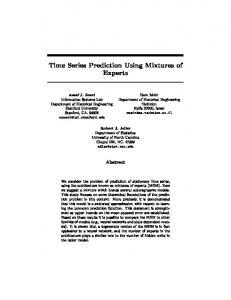
There are many applications where a system evolves differently depending on one or more external triggering “context” signals. A typical example in discrete manufacturing is a robot manipulating bottles arriving on a conveyor belt: Depending on sensor signals indicating (i) the presence of a bottle, (ii) whether the bottle is already filled or empty and (iii) which liquid to fill in, the robot starts different sequences of actions like filling liquid from different sources or ignoring already filled bottles. A controller which can be trained easily to perform these sequences depending on the sensor information represents a significant simplification for installing and reconfiguring automation systems. Here, we consider another application, namely a warehouse in figure 1(a) for many commodities which arrive at the warehouse in random order rather than regular one. When a trolley is assigned a job to convey a product to its respective cabin, a suitable sensor provides the associated information φ indicating, for example, the destination cabin for the product. During the transportation, the trajectory of trolley and product is recorded and used for on-line training of a dynamical trajectory model that, given the previous positions on a grid of suitable spatial resolution, predicts the next position. After sufficient time of learning, the model should be able to reproduce the trajectories of previously seen products given the associated φ-values. In the next section, Spiral recurrent neural network architecture is introduced for the conditional prediction problem. Section-3 and section-4 will present the simulations, results and discussion, where performance of different neural network models will be addressed. Conclusion will be given in the last section.
125
ESANN'2008 proceedings, European Symposium on Artificial Neural Networks - Advances in Computational Intelligence and Learning Bruges (Belgium), 23-25 April 2008, d-side publi., ISBN 2-930307-08-0.
2 2.1
Conditional Prediction with SpiralRNN Spiral Recurrent Neural Network
Spiral recurrent neural network (SpiralRNN) [3] is a novel neural network architecture for efficient and stable on-line time series prediction. Forward evolution of a SpiralRNN model is very similar to conventional recurrent neural networks, which follows equation (1) and equation (2). Here, x is the data whose dynamics is to be trained, s refers to the hidden state vector, H and G are the activation functions in hidden layer and output layer respectively, Win Whid and Wout are connection-weight matrices in the input, hidden and output layers, and b1 and b2 are the respective bias vectors in hidden and output layer. st+1 xt+1
H (Whid st + Win xt + b1 ) G (Wout st+1 + b2 )
= =
(1) (2)
SpiralRNN models differ from conventional RNNs in their special structure of the hidden layer weight matrix Whid , which is a block-diagonal matrix with μ sub-blocks. Each sub-block matrix Mk is determined by an associated vector (k) (k) (k) β (k) = {β1 , β2 , . . . , βu−1 }T as shown in figure 1(b), with k ∈ [1, μ] being the indices of sub-blocks and u ∈ N indicating the size of Mk . Furthermore the (k) (k) value of β satisfies the condition: βi = tanh(γi ). With the special structure as well as the squash function of vector β, the maximum absolute eigenvalue of k-th sub-block matrix is bounded as shown in equation (3). Because of the blockdiagonal structure, matrix Whid ’s maximum absolute eigenvalue λmax satisfies equation (4). |λ(k) |
u−1 �
≤
(k)
|βi | =
i=1
λmax
max {λ
=
u−1 �
(k)
|tanh(γi )| < u − 1
(3)
i=1 (k)
}
k∈[1,...,µ]
(4)
With such constraint on the eigenvalue spectrum of hidden-weight matrix, as well as the fact that matrix Whid is determined by vectors which can be optimized, SpiralRNN model enjoys the advantage of constraint eigenvalue spectrum 10 9
y(×0.1)
Postern
8 7
A
6 5 4 3 2 1
F
0
1
2
0000000 1111111 0000000 1111111 0000000 D1111111 E 0000000 1111111 0000000 1111111 C 0000000 1111111 0000000 1111111 0000000 1111111 00000000 11111111 00000000 11111111 00000000000 11111111111 B 00000000 11111111 00000000000 11111111111 00000000 11111111 00000000000 11111111111 00000000 11111111 00000000000 11111111111 00000000 11111111 00000000000 11111111111 00000000 11111111 00000000000 11111111111 00000000000 11111111111 00000000000 11111111111 00000000000 11111111111
3
4
Entrance 5 6 7
8
9
0 B B B B B B B B B Mk = B B B B B B B B @ x(×0.1) 10
β
0
(k) u−1
(k) β1
0
(k) β2
(k) β1
. . . (k) β u−1
. . . ...
β β
(k) u−2 (k) u−1
...
(k) β1
...
. . .
. 0 .
.
. .
...
.
.
.
(k) β1
(b) Structuer of sub-block Mk
(a) Schematic Diagram of warehause
. . .
. β
(k) u−1 0
1 C C C C C C C C C C C C C C C C C A u×u .
Fig- 1: (a) Schematic diagram of warehouse. Product cabins are denoted by capital letters and obstacles are in shaded area. (b) Structure of sub-block matrix Mk .
126
ESANN'2008 proceedings, European Symposium on Artificial Neural Networks - Advances in Computational Intelligence and Learning Bruges (Belgium), 23-25 April 2008, d-side publi., ISBN 2-930307-08-0.
like in echo state neural network (ESN) [1] and the advantage of rich complexity of dynamics modeling ability like in simple recurrent net (SRN) [2], and is hence suitable for on-line time series prediction. For more details, refer to [3]. 2.2
Implementation of SpiralRNN in Conditional Prediction
In the conditional prediction problem of trajectory reproduction, data tuple xt = [pt , φ] consist of the trajectory data pt (which is two dimensional in this case) and the corresponding φ-value (which is one dimensional in this case), where t ∈ [1, lp ] is the index for time step and lp is the length of the particular trajectory pattern. Here, we assume that φ is unique and constant for one particular trajectory/product; this can be realized by storing the initial trigger signal (given by sensor) until another signals terminating the trajectory, i.e. product has been conveyed to the destination. At t = 0, different trajectory patterns will be separately assigned a virtual starting point p0 . The value of p0 is different for each pattern but is randomly initialized the first time a specific pattern occurs. Initialization: Every time before training or testing with any trajectory pattern p�, the hidden-state vector of the neural network will be reset to zero in order to avoid influence from previous data sequence. More important, the tuple x0 = [p0 , φ] at time t = 0 is initialized such that p0 value is unique but constant for different product/trajectory, as is the φ value. In such a way, the starting data item of the same product/trajectory, which is to be used in training and testing, is the constant. Training: At time step t + 1, for instance, the target tuple is constructed with ˆt as the latest data: x ˆt+1 = [pt+1 ; φi ]. By setting the previous tuple x input, the neural network iterates according to equation (1) and equation ˆt in equation (1). Different from (2). By teacher forcing, xt is replaced by x batch training, the network parameters are updated each time step upon ˆt+1 . The on-line training comparing the output xt+1 with the new tuple x is based on an extended Kalman filter (EKF)[4] with a real-time recurrent learning gradient; this combination can be justified theoretically and has proven successful in earlier tests [3]. Training will be stopped as soon as the last tuple for the particular trajectory of a product is given; this can be realised by a sensor signal indicating arrival at the target position. Testing: In testing, the production type is known, so is the φ-value, and the task is to reproduce the corresponding trajectory for monitoring and diagnosis purposes. Again, the initialization step will be taken before the starting of the testing. Having the initial tuple x0 in initialization step, the neural network iterates according to equation (1) and equation (2) as it does in training step. The output of network in testing will be set as the input in the next iteration of the autonomous test. Such autonomous iterations continue until the stopping criterion is satisfied, usually the length of autonomous test lp is predefined.
127
ESANN'2008 proceedings, European Symposium on Artificial Neural Networks - Advances in Computational Intelligence and Learning Bruges (Belgium), 23-25 April 2008, d-side publi., ISBN 2-930307-08-0.
3
Experimental Settings
Data The trajectory data set is extracted from the trajectory coordinates of different products in the warehouse scenario shown in Figure 1(a). It is assumed that, in each time step, the trolley moves from one grid point to the neighbor grid point. Values of φ for trajectory patterns A to F are respectively set to {1, −1, 0.5, −0.5, 2, −2}. The initial virtual starting point p0 is randomly initialized within range (−1, 1) for different patterns. The length of each trajectory (excluding the virtual starting point) is set as lp = 11. The number of trajectories np in each simulation varies, ranging from 2 to 6. Choice of data-sequences of trajectories will orderly start from product A, e.g. trajectories of products A, B and C will be chosen when np = 3. Data are corrupted by normally distributed noise N (0, 0.012 ) with mean 0 and standard deviation 0.01. Comparison Models The performance of SpiralRNN model will be compared to that of conventional neural network models including: echo state network (ESN), block diagonal recurrent net (BDRNN)[5] and the classical multi-layer perceptron (MLP). For sake of fair comparison, number of trainable parameters (i.e. the complexity of model) in the models will keep to the same level, as the computational cost of extended Kalman filter (EKF) training is mainly dependent on this value. As the number of input/output neurons of models is dependent on the dimension of data and is therefore fixed, one can change the number of hidden nodes in order to change the complexity of the particular model. Model parameters in most cases were initialized according to the normal distribution N (0, 0.012 ). For reason of easy deployment, construction of SpiralRNN model follows [3] and number of hidden units will be the same as number of input nodes where hidden units have the same size and structure. Configuration of ESN model follows [1], in such a way that the hidden weight matrix Whid is initialized randomly over range [−1, 1] with the sparsity value 95%, afterward the matrix is rescaled such that the maximum eigenvalue of Whid is equal to 0.8. The BDRNN model will take the scaled orthogonal version, where the entries of the 2 × 2 subblock matrix is determined by two variables w1 and w2 and they satisfy w12 + w22 ≤ 1 (for details refer to [5]). Training and Testing Training was implemented in rounds, where in each round the network model was trained with all trajectory time series separately. Note that entries of the hidden state are re-set to zeros before the training with any trajectory. After each 10 rounds of such training, the trained model produces corresponding autonomous output given different initial inputs. For more details, refer to section-2.2. Evaluation Evaluation focuses on the output vector components corresponding to trajectory, namely Γ. The evaluation error ε is then calculated according
128
ESANN'2008 proceedings, European Symposium on Artificial Neural Networks - Advances in Computational Intelligence and Learning Bruges (Belgium), 23-25 April 2008, d-side publi., ISBN 2-930307-08-0.
to equation 5 and equation 6. Note that �i,t,k in equation 6 refers to taking the mean value of � over all indices i, t and k, and that when t = lp � refers to the error of lp -step-ahead prediction. The final result takes the average value over 30 simulations. �i,t,k ε
4
= (ˆ xi,t,k − xi,t,k )2 , = �i,t,k
i ∈ Γ, t ∈ [1, lp ], k ∈ [1, np ]
(5) (6)
Results
Performance result from competing models of different size in different tasks are given in table-1, where models have been trained nt = 20 rounds. Figure 2 illustrates the histogram plot of ε value over 30 simulations with np =4 training patterns and 200 parameters in model. Table-2 shows the improvement of performance of SpiralRNN model with more training data. The histogram of ε over 30 runs of 200-weights SpiralRNN model is given in figure 3. All numbers in tables are base-10 logarithm values of the respective ε. In histogram figures, Xaxis represents the value of ε with unit of 10−3 and Y-axis shows the occurrence frequency of respective ε value. Model SpiralRNN ESN BDRNN MLP
100 weights 200 weights 300 weights np =2 np =3 np =4 np =4 np =5 np =6 np =5 np =6 -3.23 -1.15 -1.52 -2.11
-2.84 -0.82 -2.17 -2.01
-2.44 -0.66 -1.98 -1.10
-3.04 -0.77 -2.25 -2.27
-2.76 -0.64 -2.24 -1.73
-2.53 -0.50 -1.97 -1.29
-2.97 -0.70 -2.27 -1.76
-2.73 -0.57 -2.23 -1.51
Table- 1: Evaluation error ε (in logarithmic scale) of models after nt = 20 training rounds in different network size in different tasks. training rounds nt =10 nt =20 nt =30 nt =40
(a) SpiralRN N
(b) M LP
Fig- 2: Histograms of ε from 200weight models with np =4 and nt =20
100 weights 200 weights 300 weights np =2 np =3 np =4 np =4 np =5 np =6 np =5 np =6 -2.76 -3.23 -3.43 -3.63
-2.46 -2.84 -3.00 -3.04
-1.99 -2.44 -2.54 -2.63
-2.47 -3.04 -3.19 -3.34
-2.23 -2.76 -2.99 -3.11
-2.03 -2.53 -2.76 -2.84
-2.39 -2.97 -3.17 -3.31
-2.02 -2.73 -3.04 -3.21
Table- 2: Evaluation error ε (in logarithmic scale) of SpiralRNN model in different network size in different tasks.
(a) nt = 10
(b) nt = 40
Fig- 3: Histograms of ε from 200weight SpiralRNN with np = 4
The results in these tables clearly show that (i) different trajectories can be stored by recurrent neural networks simultaneously and (ii) that SpiralRNN outperforms other approaches in different prediction tasks and with different size of network. It is worth mentioning that SRN shows similar or even slightly better results than SpiralRNN but sometimes suffer from instability effects such that training fails completely (see also [3]). On the other hand, this result indicates that the constraints on the hidden layer structure of a SpiralRNN do not severely constrain the modeling power of this architecture compared to the unconstrained SRN. The worse performance of ESN indicates that their reduced variability (only the output weights can be trained) imposes too many constraints. BDRNN and MLP models have achieved better results than ESN, but suffer from slow convergence. The histogram plot figure 2 illustrates the improved stability of the SpiralRNN compared with e.g. MLP.
129
ESANN'2008 proceedings, European Symposium on Artificial Neural Networks - Advances in Computational Intelligence and Learning Bruges (Belgium), 23-25 April 2008, d-side publi., ISBN 2-930307-08-0.
0.8
0.8
0.8
0.5 0.6
Auto. Output Target
Auto. Output Target
0.4
0.6
0.3
0.4
0.6
0.4
0.4
0.2 0.2
0.2
0.2
0.1
Auto. Output Target
0 0.1
0.2
0.3
0.4
(a) trajectory A
0.4
0.5
0.6
0.7
0.8
0.9
(b) trajectory B
0.4
0.5
0.6
Auto. Output Target
0
0
0
0.7
(c) trajectory C
0.4
0.45
0.5
(d) trajectory D
Fig- 4: Autonomous outputs on np = 4 trajectory patterns from 200-weight SpiralRNN model after nt = 20 training rounds.
Typical examples of trajectory prediction by SpiralRNN are given in figure 4. Note that in each sub-plot the output trajectory is the autonomous result given initial starting value but no further data input. Increasing the number of trajectories to be predicted will generally require either longer training time or larger neural network model in order to obtain the same level of performance. Table-2 reports the performance of a SpiralRNN architecture of different network size and in different prediction tasks with varying number of trajectory patterns. Figure 3 which compares the histogram of error from SpiralRNN model at nt = 10 training rounds and that at nt = 40 has confirmed the convergence of learning. Because of the grid, one prediction can be consider to be matched if the absolute prediction error is smaller than 0.05, therefore the threshold value is defined as θ = log 10(0.052 ) � −2.6. It is shown in table-2 that, after nt = 20 or even nt = 10 training rounds, SpiralRNN model is able to achieve an evaluation error smaller or close to this threshold in all mentioned tasks.
5
Conclusion
This paper addresses the conditional prediction of data time series with a SpiralRNN model. We simulate the problem with a warehouse scenario where a trigger signal depending on product type and thus destination provides a value of the additional input φ. The task is to reproduce the trajectory of transportation of the respective product. SpiralRNN model has proven successful in such conditional prediction tasks compared to other state-of-the-art approaches.
References [1] Herbert Jaeger. Adaptive nonlinear system identification with echo state networks. Advances in Neural Information Processing Systems, 15:593–600, 2003. [2] Jeffrey L. Elman. Finding structure in time. Cognitive Science, 14(2):179–211, 1990. [3] Huaien Gao, Rudolf Sollacher, and Hans-Peter Kriegel. Spiral recurrent neural network for online learning. In 15th European Symposium On Artificial Neural Networks Advances in Computational Intelligence and Learning, Bruges (Belgium), April 2007. [4] F.L. Lewis. Optimal Estimation: With an Introduction to Stochastic Control Theory. A Wiley-Interscience Publication, 1986. ISBN: 0-471-83741-5. [5] P.A. Mastorocostas and J.B. Theocharis. On stable learning algorithm for block-diagonal recurrent neural networks, part 1: the RENNCOM algorithm. IEEE International Joint Conference on Neural Networks, 2:815– 820, 2004.
130