International Journal of Computational and Theoretical Statistics ISSN (2210-1519) Int. J. Comp. Theo. Stat. 5, No. 1 (May-2018) http://dx.doi.org/10.12785/ijcts/050101
Confidence Intervals based on Absolute Deviation for Population Mean of a Positively Skewed Distribution Moustafa Omar Ahmad Abu-Shawiesh1, Shipra Banik2 and B.M. Golam Kibria 1 Department of Mathematics, Hashemite University, Al-Zarqa 13115, JORDAN Department of Physical Sciences, Independent University, Bangladesh, Dhaka 1212, BANGLADESH 3 B.M. Golam Kibria, Department of Mathematics and Statistics, Florida International University, Miami, FL 33199, USA 2
Received September 30, 2017, Revised December18, 2017 Accepted January 23, 2018, Published May 1, 2018 Abstract: This paper proposes three alternative confidence intervals namely, AADM-t, MAAD-t and MADM-t, which are simple adjustments to the Student-t confidence interval for estimating the population mean of a positively skewed distribution. The proposed methods are very easy to calculate and are not overly computer-intensive. The performance of these confidence intervals was compared through a simulation study using the following criterion: (a) coverage probability (b) average width and (c) coefficient of variation of width. Simulation studies indicate that for small sample sizes and moderate/highly positively skewed distributions, the proposed AADM-t confidence interval performs the best and it is as good as the Student-t confidence interval. Some real-life data are analyzed which support the findings of this paper to some extent. Keywords: Confidence interval, Robustness, Absolute deviation, Coverage probability, Positively skewed distribution, Monte Carlo simulation.
1.
INTRODUCTION
The positively skewed data are frequently encountered in both economics and health-care fields where experiments with rare diseases or a typical behavior are the norm. The classical Student-t confidence interval is the most widely classical used approach because it is simple to calculate and robust for both small and large sample sizes. However when the population distribution is positively skewed, the Student-t confidence interval will only have an approximate (1-α) coverage probability. This coverage probability may be improved by developing different confidence interval methods in order to analyze the positively skewed data. This paper reviews and develops some confidence intervals which handle both small samples and positively skewed data. Since a theoretical comparison among the interval is not possible, a simulation study has been conducted to compare the performance of the intervals. The coverage probability (CP), average width (AW) and coefficient of variation of widths (CVW) are considered as a performance criterion. They have been recorded and compared across confidence intervals. Smaller width indicates a better confidence interval when coverage probabilities are the same. Higher coverage probability indicates a better confidence interval when widths are the same. This paper is organized as follows: The proposed confidence intervals have been developed in section 2. A Monte Carlo simulation study has been conducted in section 3. As applications, some real life data have been analyzed in section 4. Some concluding remarks are given in section 5. 2.
THE PROPOSED CONFIDENCE INTERVAL ESTIMATORS
The main characteristics for the scale estimators based on the median absolute deviation for constructing the proposed confidence intervals will be discussed in this section. Let X1, X2, … , Xn be a random sample which is independently and identically distributed and comes from a positively skewed distribution with unknown μ and σ. We want to develop 100(1-α)% confidence interval for μ. The classical Student-t confidence interval for μ and the proposed median absolute deviations confidence intervals have been discussed as below:
E-mail address:
[email protected],
[email protected] and
[email protected] http://journals.uob.edu.bh
2
M. Abu-Shawiesh, et. al.: Confidence Intervals based on Absolute Deviation for Population…
A. The classical Student-t confidence interval This interval relies on the normality assumption and is developed by [1] as a more robust way for testing hypotheses specifically for small sample sizes and/or σ is unknown. The (1–α)100% confidence interval for μ can be constructed as follows: , (1) X Z
2
n
when σ is known. For small sample sizes and unknown σ, the (1–α)100% confidence interval for μ which is known as the Student-t confidence interval can be constructed as follows: X t
, n 1 2
where t(
2 , n 1)
(2)
S , n
is the upper α/2 percentage point of the student t distribution with (n-1) degrees of freedom. The
classical Student-t approach is not very robust under extreme deviations from normality [2]. Additionally, since the classical Student-t depends on the normality assumption, it may not be the best confidence interval for asymmetric distributions. In this paper, we assume that X follows a positively skewed distribution. Previous researchers have found that the Student-t performs well for small samples sizes and asymmetric distributions in terms of the coverage probability coming close to the nominal confidence coefficient although its average widths and variability were not as small as other confidence intervals ([2]-[5]). B. The Proposed Median Absolute Deviations Confidence Intervals For a positively skewed distribution, it is known that the median describes the center of a distribution better than the mean. Thus for a positive skewed data and because of the robustness of the median, in this section, we will consider three methods based on median absolute deviations statistics to construct the confidence interval for μ. The proposed confidence intervals are computationally simple and therefore analytically a more desirable methods. C. The AADM-t Confidence Interval The first method we propose in this paper is called the AADM-t confidence interval, which is a modification of the classical Student-t confidence interval. The (1–α)100% AADM-t confidence interval for μ is given by: X t
, n 1 2
(3)
AADM , n
n where AADM 2 X i MD , MD is the sample median. As stated in [6], if X1, X2, … , Xn ~ N(μ,2), then n i 1
AADM is a consistent estimate of σ and is asymptotically normally distributed, which is:
lim E ( AADM )
n
n ( AADM ) N (0 ,
1) 2
Moreover, using the strong law large numbers, it can be shown that AADM converges to σ almost surely. D. The MAAD-t Confidence Interval The second method we propose in this paper is called the MAAD-t confidence interval, which is another modification of the classical Student-t confidence interval. The (1–α)100% MAAD-t confidence interval for μ is given by:
http://journals.uob.edu.bh
Int. J. Comp. Theo. Stat. 5, No. 1, 1-13 (May-2018) (4)
MAAD , n
X t
, n 1 2
3
where MAAD is defined as
MAAD median
X
i
X
, i 1, 2,..., n
(5)
This estimator was given by [7] and they showed that it is more robust than S. E.The MADM-t Confidence Interval The third method we propose in this paper is called the MADM-t confidence interval, which is another modification of the classical Student-t confidence interval. This method is based on MADM. The (1–α)100% MADM-t confidence interval for μ is given by: (6) MADM , X t , n 1 2
n
where MADM was first introduced by [8] and is defined as
MADM median
X
i
MD , i 1, 2, ... , n
(7)
The MADM has important robustness properties as follows: (i) It has a maximum breakdown point which is 50% which is twice as much as interquartile range (IQR) (ii) It has the smallest gross error sensitivity value which is 1.167. (iii) It has the sharpest bound of influence function. (iv) The efficiency of it is 37% for the case of normal distribution. (v) If the MADM is multiplied by 1.4826, it becomes an unbiased estimator of σ. 3. SIMULATION STUDY Since a theoretical comparison among the intervals is difficult, following [3], a simulation study has been conducted to compare the performance of the confidence intervals. Based on the results of the simulation studies, the best confidence interval will be chosen based on coverage probability (CP), average width (AW), coefficient of variation of the widths (CVW), sample size (n) and skewness level. The program for the simulation study has been conducted using MATLAB(2015) programming languages. Since our main objective is to compare the performance of the classical Student-t and the proposed confidence intervals for positive skewed distributions, then to generate data, we choose the gamma distribution with various skewness levels for comparison purposes. The probability density function of the gamma distribution is defined as f (x / , )
1 ( )
x 1 exp(
x
)
where α is a shape parameter and β is a scale parameter. The mean of this distribution is and variance is 2 2 . We want to find some good confidence intervals which will be useful for a sample coming from a positively skewed distribution. A. The Simulation Technique The program flowchart for the simulation study is as follows: (i) Select the sample size (n), number of simulation runs (M) and the confidence significance level (α). (ii) Generate a random sample of size (n), X1, X2, … , Xn, which is an independently and identically distributed and comes from a gamma distribution with two parameters α and β with the chosen population skewness using the MATLAB (2015) program. (iii) Construct confidence intervals at a (1-α)100% confidence level using the formulas defined in section 2. (iv) For each confidence interval constructed, determine if the confidence interval includes µ and for those confidence intervals that contain the mean calculate the width of the confidence interval.
http://journals.uob.edu.bh
4
M. Abu-Shawiesh, et. al.: Confidence Intervals based on Absolute Deviation for Population… (v) Repeat (i)-(iv) M times, then compute CP (the proportion of intervals that contain the true mean out of M intervals), AW and CVW(ratio of coverage to width).
Following [3], the parameters for the gamma distribution have been chosen and the random sample of size n, X1, X2, ..., Xn was taken from the following gamma distributions with a common mean of 10: (a) G(16,0.625) with skewness 0.5; (b) G(4,2.5) with skewness 1; (c) G(1,10) with skewness 2; (d) G(0.25,40) with skewness 4; (e) G(0.11,40) with skewness 6; (f) G(0.063,40) with skewness 8. To check whether our selected four methods are sensitive with n or not, we choose n from 5 to 100. The confidence level for the simulation study is 0.95 which is the common confidence interval. The number of M was chosen to be 2500. More on simulation techniques, we refer [9] -[10] among others. B. The Simulation Results CP, AW and CVW for selected n and for skewness 0.5, 1, 2, 4, 6, and 8 are calculated and given in Tables I-VI respectively and in figures 1-6 respectively. TABLE I. ESTIMATED COVERAGE PROBABILITIES USING GAMMA (16,0.625) WITH SKEWNESS = 0.5 Student-t
AADM-t
MAAD-t
MADM-t
n CP
AW
CVW
CP
AW
CVW
CP
AW
CVW
CP
AW
CVW
5
0.867
29.03
67.32
0.838
23.96
63.61
0.781
19.33
67.23
0.583
11.30
85.14
6
0.900
28.45
60.83
0.882
23.91
55.76
0.827
18.51
57.92
0.654
11.24
69.50
7
0.829
17.80
57.69
0.794
14.73
52.82
0.715
11.62
56.77
0.497
6.98
73.00
0.824
14.83
49.70
0.746
11.44
52.32
0.536
7.00
63.87
0.842
14.56
47.00
0.758
11.31
50.56
0.539
6.81
62.53
11.03
45.82
0.576
6.80
56.72
10.97
43.72
0.592
6.71
56.18
0.820
10.76
42.38
0.614
6.58
51.02
0.722
8.08
41.64
0.497
4.86
52.22
8.04
38.89
0.536
4.85
48.16
0.542
4.87
46.98
8
0.850
17.68
9
0.872
17.60
55.02 52.18
0.860
14.44
42.81
0.879
13.80
10
0.890
17.34
47.74
11
0.907
17.13
45.42
0.882
14.05
10.97 39.48
0.830
10.50
38.49
10.54
36.06
0.754
7.99
37.54
0.812
7.88
32.64
0.582
4.74
40.83
0.540
3.77
36.71
12
0.911
16.88
44.22
13
0.868
12.69
44.02
14
0.885
0.785 0.806
12.77
41.22
0.856
10.43
34.38
0.898
10.35
30.24
0.773
6.21
28.78
0.790
6.16
27.12
0.556
3.73
33.25
0.521
3.12
31.08
0.852
0.751
15
0.887
12.67
39.63
20
0.927
12.66
35.26
0.876
8.15
26.63
0.887
8.13
24.88
0.772
5.14
24.82
0.790
5.15
23.41
0.558
3.10
29.59
0.509
2.63
26.50
25
0.914
9.96
31.74
30
0.934
10.00
29.89
0.866
6.76
22.53
0.891
6.78
21.34
0.745
4.36
21.60
35
0.909
8.27
26.90
40
0.935
8.36
25.38
0.863
5.75
20.17
0.884
5.74
18.60
0.778
4.35
20.23
0.539
2.63
26.04
5.01
17.54
0.748
3.79
19.09
0.510
2.30
23.04
0.796
3.80
17.21
0.567
2.30
21.42
0.757
3.36
16.29
0.512
2.04
20.64
0.552
2.04
19.28
0.534
1.82
18.58
45
0.919
7.09
24.99
50
0.934
7.07
22.63
60
0.921
6.18
21.53
0.894
5.01
16.09
0.871
4.43
15.09
0.788
3.35
15.27
0.760
3.00
14.54
0.861
70
0.939
6.19
20.49
80
0.933
5.50
18.76
0.898
4.43
13.96
0.881
3.97
13.36
90
0.952
5.49
17.37
100
0.927
4.93
16.86
http://journals.uob.edu.bh
Int. J. Comp. Theo. Stat. 5, No. 1, 1-13 (May-2018)
Student-t
AADM-t
MAAD-t
5
MADM-t
1 0.95 0.9 0.85 0.8 0.75 0.7 0.65 0.6 0.55 0.5 0.45 0.4 0
5 10 15 20 25 30 35 40 45 50 55 60 65 70 75 80 85 90 95 100
Figure 1. Estimated Coverage Probabilities using Gamma (16, 0.625) with Skewness = 0.5
From Table I and Fig.1, we observe that the classical Student-t confidence interval has coverage probability close to the nominal level, followed by AADM-t and MAAD-t confidence intervals. It is also observable that, MAAD and MADM have the smallest widths as compare to other two selected confidence intervals. TABLE II.
ESTIMATED COVERAGE PROBABILITIES USING THE GAMMA (4, 2.5) WITH SKEWNESS = 1.0 Student-t
AADM-t
MAAD-t
MADM-t
n CP
AW
CVW
CP
AW
CVW
CP
AW
CVW
CP
AW
CVW
5
0.934
15.83
46.23
0.914
13.72
44.33
0.832
10.54
52.62
0.740
8.47
61.83
6
0.954
15.02
41.18
0.939
13.63
39.93
0.866
10.22
46.27
0.793
8.22
51.53
7
0.906
9.79
38.27
0.887
8.77
36.32
0.778
6.73
44.49
0.688
5.56
50.19
0.904
8.60
33.96
0.807
6.39
40.75
0.730
5.34
44.57
0.918
18.87
31.46
0.820
13.98
39.27
0.756
11.92
43.05
0.826
13.77
36.64
0.768
11.72
39.97
0.847
13.80
36.81
0.782
11.90
39.73
0.797
11.73
35.77
8
0.920
9.38
35.45
9
0.932
20.75
33.97
0.930
18.86
29.80
0.934
18.74
28.74
0.853
13.64
34.10
0.755
10.06
32.92
0.688
8.68
35.63
0.728
8.59
32.94
10
0.945
20.44
31.99
11
0.947
20.33
30.17
0.950
18.73
27.36
0.892
13.78
25.99
0.782
9.90
31.16
0.732
8.70
33.66
0.789
8.56
28.23
12
0.960
20.26
29.66
13
0.908
14.98
28.41
0.902
13.69
24.85
13.70
24.18
0.796
9.91
0.843
9.71
31.10 26.61
0.805
7.68
24.33
0.756
6.82
25.31
0.803
6.83
23.06 21.49
14
0.917
14.75
26.91
15
0.929
14.75
0.917 0.950
13.61
20.84
20
0.960
14.57
26.56 22.90
25
0.942
11.48
20.40
0.930 0.952
10.75
18.48
10.80
16.99
0.844
7.68
22.30
0.917
8.90
15.89
0.788
6.30
20.81
0.744
30
0.964
11.51
18.78
35
0.933
9.48
17.69
40
0.948
9.39
16.45
0.938
8.84
0.823
6.25
0.777
5.64 5.61
45
0.937
8.11
15.74
0.924
7.63
14.23 13.97
19.15
0.779
5.39
18.37
0.729
4.82
20.01 18.30
50
0.947
8.09
14.40
0.936
7.62
12.83
0.818
5.38
16.80
0.770
4.82
17.39
60
0.935
7.07
13.28
0.922
6.66
11.82
0.800
4.69
15.64
0.749
4.23
15.87
0.952
6.66
10.87
0.821
4.70
14.23
0.787
4.22
14.78
0.924
5.89
10.19
0.802
4.15
13.58
0.755
3.72
13.83
0.824
4.13
12.66
0.782
3.73
13.07
0.796
3.72
12.33
0.745
3.35
12.57
70
0.960
7.06
12.21
80
0.935
6.25
11.58
0.946
5.88
9.63
0.934
5.30
9.30
90
0.958
6.23
11.07
100
0.945
5.61
10.69
http://journals.uob.edu.bh
6
M. Abu-Shawiesh, et. al.: Confidence Intervals based on Absolute Deviation for Population…
Student-t
AADM-t
MAAD-t
MADM-t
1 0.95 0.9 0.85 0.8 0.75 0.7 0.65 0.6 0
5 10 15 20 25 30 35 40 45 50 55 60 65 70 75 80 85 90 95 100
Figure 2. Estimated Coverage Probabilities using the Gamma (4, 2.5) with Skewness = 1.0
From Table II and Fig.2, we observe that when skewness increases from 0.5 to 1.0, our proposed AADM-t confidence interval followed by MAAD-t confidence interval coverage probabilities are close to the nominal level with the classical Student-t confidence interval. Smallest widths are observed from our two proposed MAAD and MADM intervals. TABLE III:
ESTIMATED COVERAGE PROBABILITIES USING THE GAMMA (1,10) WITH SKEWNESS = 2.0
Student-t
n
AADM-t
MAAD-t
MADM-t
CP
AW
CVW
CP
AW
CVW
CP
AW
CVW
CP
AW
CVW
5
0.939
8.546
46.59
0.913
31.33
45.00
0.840
24.33
54.00
0.758
19.73
62.25
6
0.960
34.02
41.35
0.948
30.79
39.62
0.874
23.10
46.00
0.798
18.44
51.06
7
0.961
33.74
41.32
0.949
30.54
39.83
0.883
22.90
45.39
0.812
18.48
50.37
8
0.916
21.15
36.08
0.905
19.44
34.30
0.794
14.43
40.57
0.707
12.02
44.09
9
0.928
20.88
33.18
0.910
19.03
31.51
0.802
14.05
39.72
0.732
12.09
43.37
10
0.935
20.39
32.82
0.922
18.83
30.53
0.827
13.80
37.00
0.757
11.77
38.90
11
0.952
20.27
30.21
0.943
18.64
28.19
0.848
13.71
36.04
0.788
11.77
38.89
12
0.960
20.03
29.37
0.952
18.58
27.04
0.863
13.48
33.61
0.803
11.71
35.49
13
0.917
15.02
27.52
0.897
13.85
25.67
0.769
10.00
33.01
0.706
8.74
35.71
14
0.921
14.86
27.26
0.909
13.81
25.00
0.784
9.98
31.19
0.724
8.72
33.45
15
0.932
14.80
25.31
0.916
13.70
23.60
0.787
9.87
31.10
0.734
8.68
32.99
20
0.958
14.50
23.07
0.952
13.57
20.89
0.840
9.71
26.28
0.795
8.61
27.35
25
0.945
11.59
20.54
0.934
10.85
18.59
0.812
7.74
24.57
0.756
6.85
25.32
30
0.957
11.47
18.55
0.950
10.76
16.76
0.837
7.59
21.74
0.799
6.78
22.58
35
0.946
9.51
17.13
0.932
8.94
15.24
0.807
6.37
20.35
0.759
5.68
21.15
40
0.953
9.48
16.28
0.942
8.92
14.61
0.838
6.31
18.94
0.786
5.64
19.53
45
0.941
8.14
15.46
0.923
7.65
13.58
0.795
5.41
18.27
0.753
4.84
18.70
50
0.947
8.09
14.40
0.936
7.62
12.83
0.818
5.38
16.80
0.770
4.53
17.39
60
0.935
7.07
13.28
0.922
6.66
11.82
0.800
4.69
15.64
0.749
4.23
15.87
70
0.954
7.05
12.62
0.945
6.64
11.07
0.827
4.68
14.43
0.778
4.20
14.43
80
0.946
6.24
11.85
0.936
5.88
10.42
0.796
4.14
13.83
0.754
3.73
13.78
90
0.963
6.21
10.59
0.954
5.87
9.37
0.841
4.13
12.51
0.792
3.72
12.88
100
0.942
5.60
10.40
0.928
5.28
9.22
0.802
3.71
12.34
0.758
3.34
12.74
http://journals.uob.edu.bh
Int. J. Comp. Theo. Stat. 5, No. 1, 1-13 (May-2018)
Student-t
AADM-t
MAAD-t
7
MADM-t
1 0.95 0.9 0.85 0.8 0.75 0.7 0.65 0.6 0
5 10 15 20 25 30 35 40 45 50 55 60 65 70 75 80 85 90 95 100
Figure 3. Estimated Coverage Probabilities using the Gamma (1, 1.0) with Skewness = 2.0
From Table III and Fig.3, it is noticeable that our proposed AADM-t and Student-t confidence interval have similar coverage probability. Intervals with respect to width are performing best as compare to the student’s t interval. TABLE IV. n
ESTIMATED COVERAGE PROBABILITIES USING THE GAMMA (0.25,40) WITH SKEWNESS = 4.0 Student-t
AADM-t
MAAD-t
MADM-t
CP
AW
CVW
CP
AW
CVW
CP
AW
CVW
CP
AW
CVW
5
0.962
4.07
37.65
0.944
3.59
38.78
0.859
2.72
48.85
0.783
2.39
59.33
6
0.975
3.82
33.32
0.964
3.53
34.76
0.896
2.6443
13.02
0.834
2.27 47.
47.86
7
0.918
2.45
29.77
0.898
2.25
31.01
0.774
1.68
41.88
0.720
1.50
47.70
8
0.936
2.41
27.17
0.920
2.26
28.33
0.809
1.65
36.45
0.754
1.47
41.11
9
0.950
2.36
25.34
0.936
2.21
26.41
0.824
1.61
36.56
0.782
1.48
41.32
10
0.961
2.30
24.19
0.948
2.19
25.19
0.842
1.57
33.51
0.799
1.45
37.34
11
0.966
2.29
23.07
0.958
2.17
23.79
0.850
1.54
33.04
0.820
1.45
36.67
12
0.970
2.27
21.62
0.961
2.17
22.77
0.867
1.55
31.09
0.839
1.45
33.13
13
0.928
1.69
20.95
0.912
1.61
21.83
0.783
1.13
30.78
0.748
1.08
33.27
14
0.941
1.67
19.81
0.932
1.61
20.60
0.806
1.14
28.58
0.780
1.08
30.63
15
0.941
1.66
19.57
0.935
1.60
20.62
0.808
1.13
29.47
0.785
1.08
31.36
20
0.964
1.63
17.02
0.961
1.58
17.57
0.841
1.10
24.89
0.828
1.06
26.23
25
0.968
1.64
16.59
0.944
1.25
15.41
0.811
0.87
22.46
0.800
0.85
23.43
30
0.968
1.27
13.60
0.965
1.25
14.10
0.843
0.86
20.72
0.834
0.84
21.34
35
0.942
1.05
12.57
0.937
1.03
13.12
0.800
0.71
19.34
0.786
0.69
19.86
40
0.954
1.05
11.94
0.953
1.04
12.32
0.832
0.71
18.04
0.826
0.69
18.34
45
0.934
0.90
10.72
0.932
0.89
11.28
0.805
0.61
16.92
0.794
0.59
17.26
50
0.948
0.90
10.36
0.946
0.89
10.87
0.815
0.61
16.24
0.808
0.60
16.79
60
0.937
0.78
9.71
0.935
0.77
9.97
0.804
0.53
14.77
0.802
0.52
15.14
70
0.954
0.78
9.01
0.951
0.77
9.34
0.825
0.52
13.89
0.814
0.52
13.96
80
0.948
0.69
8.37
0.945
0.69
8.72
0.818
0.47
12.71
0.813
0.46
12.96
90
0.956
0.69
7.89
0.955
0.69
8.17
0.824
0.47
12.24
0.818
0.46
12.22
100
0.952
0.62
7.32
0.949
0.61
7.66
0.817
0.42
11.64
0.808
0.41
11.91
http://journals.uob.edu.bh
8
M. Abu-Shawiesh, et. al.: Confidence Intervals based on Absolute Deviation for Population…
Student-t
AADM-t
MAAD-t
MADM-t
1 0.95 0.9 0.85 0.8 0.75 0.7 0.65 0.6 0
5 10 15 20 25 30 35 40 45 50 55 60 65 70 75 80 85 90 95 100
Figure 4. Estimated Coverage Probabilities using the Gamma (1, 1.0) with Skewness = 4.0
From Table IV and Fig.4, we observe that in case of a moderate to highly skewed distribution, the AADM-t confidence interval coverage probability is very close to nominal level 0.95 as compare to others. Here also our proposed intervals performing very well. TABLE V. n
CP
5
0.962
6
0.982
7
Student-t AW
ESTIMATED COVERAGE PROBABILITIES USING THE GAMMA (0.11,40) WITH SKEWNESS = 6 CVW
CP
1.79
36.82
0.946
1.67
33.38
0.971
0.920
1.09
30.56
8
0.947
1.06
9
0.951
1.03
10
0.960
1.01
11
0.966
1.00
12
0.976
13
0.926
14 15
AADM-t AW
CVW
CP
1.58
37.63
0.852
1.55
34.95
0.895
0.897
1.01
31.55
27.24
0.930
1.00
26.18
0.938
0.94
23.90
0.95
23.06
0.956
1.00
21.83
0.74
21.31
0.938
0.73
0.940
0.73
20
0.966
25 30
MAAD-t AW
MADM-t AW
CVW
CP
CVW
1.19
48.30
0.784
1.05
8.57
1.15
42.77
0.846
1.00
47.71
0.780
0.76
41.49
0.720
0.68
46.66
28.05
0.814
0.73
36.26
0.756
0.65
40.71
27.29
0.809
0.69
37.39
0.764
0.65
42.46
0.96
24.76
0.841
0.69
32.84
0.812
0.64
36.06
0.95
24.01
0.854
0.68
34.14
0.822
0.64
37.16
0.968
0.96
23.09
0.873
0.68
31.71
0.844
0.64
34.09
0.914
0.71
21.95
0.783
0.50
31.03
0.751
0.47
33.27
20.23
0.924
0.70
20.98
0.798
0.49
28.97
0.766
0.47
31.06
19.79
0.934
0.70
20.47
0.804
0.49
28.89
0.779
0.47
30.95
0.71
16.96
0.960
0.69
17.68
0.852
0.47
25.15
0.840
0.46
26.35
0.950
0.56
15.10
0.944
0.55
15.65
0.814
0.38
23.03
0.804
0.37
24.03
0.966
0.56
13.77
0.959
0.55
14.37
0.837
0.37
20.40
0.823
0.36
21.04
35
0.955
0.46
12.72
0.958
0.45
13.23
0.814
0.31
19.54
0.809
0.32
20.55
40
0.960
0.46
12.08
0.954
0.45
12.58
0.829
0.31
18.45
0.813
0.30
18.90
45
0.942
0.39
10.74
0.938
0.39
11.20
0.793
0.26
17.06
0.785
0.26
17.22
50
0.944
0.39
10.44
0.941
0.39
10.88
0.815
0.26
16.30
0.804
0.26
16.52
60
0.946
0.34
9.44
0.942
0.34
9.70
0.800
0.23
14.44
0.793
0.22
14.74
70
0.955
0.34
8.74
0.955
0.34
9.08
0.833
0.23
13.59
0.826
0.22
13.90
80
0.950
0.30
8.25
0.947
0.30
8.63
0.861
0.20
13.08
0.817
0.20
13.38
90
0.953
0.30
7.64
0.953
0.30
7.97
0.829
0.20
12.30
0.815
0.20
12.40
100
0.954
0.27
7.40
0.953
0.27
7.62
0.824
0.18
11.41
0.812
0.18
11.70
http://journals.uob.edu.bh
Int. J. Comp. Theo. Stat. 5, No. 1, 1-13 (May-2018)
Student-t
AADM-t
MAAD-t
9
MADM-t
1 0.95 0.9 0.85 0.8 0.75 0.7 0.65 0.6 0
5 10 15 20 25 30 35 40 45 50 55 60 65 70 75 80 85 90 95 100
Figure 5. Estimated Coverage Probabilities using the Gamma (1, 1.0) with Skewness = 6.0
From Tables V-VI and Fig.5 and Fig. 6 we observe that in case of a very highly skewed distribution, the AADM-t confidence interval coverage probability is stable and very close to the nominal level 0.95 as compare to others. Here also our proposed intervals performing very well in terms of widths when the sample sizes are small. TABLE VI.
ESTIMATED COVERAGE PROBABILITIES USING THE GAMMA (0.063,40) WITH SKEWNESS =8
Student-t
AADM-t
n
CP
AW
CVW
CP
AW
5
0.962
0.97
36.83
0.946
0.86
6
0.978
0.93
32.26
0.970
0.86
7
0.928
0.59
29.59
0.904
31 0.54
8
0.934
0.57
27.79
0.919
0.54
9
0.951
0.56
26.18
0.938
0.52
10
0.960
0.55
23.90
0.953
0.52
11
0.966
0.55
23.06
0.956
0.52
12
0.976
0.54
21.83
0.968
0.52
13
0.926
0.40
21.31
0.914
14
0.938
0.40
20.23
15
0.940
0.40
19.26
20
0.969
0.39
25
0.956
0.31
30
0.971
35
0.947
40
MAAD-t
MADM-t
CVW
CP
AW
CVW
CP
AW
CVW
37.63
0.852
0.65
48.30
0.780
0.57 5
58.53
0.892
0.64
41.79
0.830
0.55
47.35
35 .07
0.776
0.40
42.28
0.71
0.36
48.72
28.88
0.797
0.39
36.99
0.751
0.36
41.31
27.29
0.808
0.38
37.39
0.764
0.35
42.46
24.76
0.845
0.37
32.84
0.845
0.37
32.84
24.01
0.854
0.37
34.14
0.825
0.35
37.16
23.09
0.870
0.37
31.71
0.844
0.35
34.09
0.38
21.95
0.784
0.27
31.03
0.751
0.26
33.27
0.924
0.38
20.98
0.792
0.27
28.97
0.766
0.25
31.06
0.932
0.38
19.93
0.790
0.26
28.70
0.768
0.25
30.74
16.65
0.963
0.38
17.38
0.857
0.26
24.63
0.840
0.25
25.83
14.49
0.949
0.30
15.11
0.819
0.21
22.52
0.812
0.10
23.40
0.30
13.48
0.965
0.30
14.12
0.846
0.20
20.76
0.835
0.10
21.34
0.25
12.42
0.941
0.25
12.97
0.807
0.17
19.12
0.801
0.08
19.91
0.965
0.25
11.75
0.962
0.24
12.15
0.830
0.17
18.12
0.823
0.08
18.58
45
0.943
0.21
11.05
0.938
0.21
11.51
0.790
0.14
17.11
0.780
0.07
17.45
50
0.954
0.21
10.56
0.955
0.21
10.98
0.826
0.14
16.09
0.815
0.07
16.44
60
0.953
0.18
9.53
0.926
0.18
9.82
0.782
0.12
14.56
0.777
0.06
14.65
70
0.956
0.18
8.79
0.951
0.18
9.08
0.834
0.12
13.49
0.828
0.06
13.68
80
0.948
0.16
8.07
0.945
0.16
8.46
0.818
0.11
13.01
0.813
0.05
13.15
90
0.956
0.16
7.79
0.954
0.16
8.13
0.833
0.11
12.16
0.825
0.05
12.41
100
0.939
0.15
7.24
0.936
0.14
7.99
0.804
0.10
11.72
0.800
0.05
11.80
33.82
http://journals.uob.edu.bh
10
M. Abu-Shawiesh, et. al.: Confidence Intervals based on Absolute Deviation for Population…
Student-t
AADM-t
MAAD-t
MADM-t
1 0.9 0.8 0.7 0.6 0
5 10 15 20 25 30 35 40 45 50 55 60 65 70 75 80 85 90 95 100
Figure 6. Estimated Coverage Probabilities using the Gamma (1, 1.0) with Skewness = 8.0
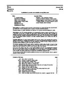
4. APPLICATIONS As an application, three examples have been considered to illustrate the performance of the confidence intervals which have been considered in this paper. These examples have various sample sizes and level of skewness. MATLAB(2015) programming language codes are used to produce necessary tables and figures respectively. A. Example-1 To study the average use of psychotropic drugs from non-antipsychotic drug users, the number of users of psychotropic drugs was reported for 20 different categories of drugs [11]. The following data represent the number of users: 43.4, 24, 1.8, 0, 0.1, 170.1, 0.4, 150.0, 31.5, 5.2, 35.7, 27.3, 5, 64.3, 70, 94, 61.9, 9.1, 38.8, 14.8. We want to find the average number of users of psychotropic drugs for non-antipsychotic drug users. The number of user is positively skewed with skewness = 1.57 and mean = 42.37. A histogram of the data values showing its positive skewness is given in Fig.7. The proposed confidence intervals and their corresponding widths have been given in Table VII. Histogram of Psychotropic Drug Exposure Data 7 6
Frequency
5 4 3 2 1 0
0
40
80
120
160
Psychotropic Drug
Figure 7. Histogram of Psychotropic Drug Exposure Data
http://journals.uob.edu.bh
Int. J. Comp. Theo. Stat. 5, No. 1, 1-13 (May-2018) TABLE VII.
11
THE 95% CONFIDENCE INTERVALS FOR PSYCHOTROPIC DRUG EXPOSURE DATA
Method
Confidence Interval
Width
Student-t
(19.748, 65.052)
45.304
AADM-t
(22.692, 62.108)
39.416
MAAD-t
(26.149, 56.651)
30.502
MADM-t
(30.232, 54.568)
24.336
We observe that the MADM-t confidence interval has the smallest width followed by MAAM-t and AADM-t. The classical Student-t confidence interval has the highest width. Both the proposed MAAD-t and MADM-t has the shorter widths compared to the corresponding AADM-t. All the confidence intervals have approximately short width. Note that the sample size n is small and data are highly skewed. Thus the MADM-t confidence interval performs the best in the sense of having smaller width than the other two proposed confidence intervals. B. Example-2 To study the Mosquito survival rates in a wet climate, 8 survival times were reported [12], the following data represents the time of death: 0.539, 0.292, 0.090, 0.044, 0.010, 0.010, 0.010, 0.031. We want to find the average survival time. Survival rate is positively skewed with skewness = 1.83 and mean is 0.13. A histogram of the data values showing its positive skewness is given in Fig.8. The proposed confidence intervals and their corresponding widths have been given in Table VIII. We found that from the Table VIII, the MADM-t confidence interval has the smallest width followed by MAAM-t and AADM-t. The classical Student-t confidence interval has the highest width. Both the proposed MAAD-t and MADM-t Histogram of Mosquito Survival Rates 5
Frequency
4
3
2
1
0 0.0
0.1
0.2 0.3 Mosquito Survival Rates
0.4
0.5
Figure 8. Histogram of mosquito survival rates data
TABLE VIII.
THE 95% CONFIDENCE INTERVALS FOR MOSQUITO SURVIVAL RATES DATA
Method
Confidence Interval
Width
Student-t
(- 0.031, 0.288)
0.319
AADM-t
(0.010, 0.247)
0.237
MAAD-t
(0.029, 0.227)
0.198
MADM-t
(0.105, 0.151)
0.046
has the shorter widths compared to the corresponding AADM-t. Here n is small and data is highly skewed. So, the MADM-t confidence interval performs the best in the sense of having smaller width than the other two proposed confidence intervals.
http://journals.uob.edu.bh
12
M. Abu-Shawiesh, et. al.: Confidence Intervals based on Absolute Deviation for Population…
C. Example-3 The percentage of adults living with HIV-1 for 15 regions of the world were reported [13], the following data represent the HIV-1 prevalence rate for each region: 0.6, 2.3, 0.6, 0.3, 0.7, 0.9, 0.3, 0.1, 0.2, 0.3, 4.5, 5.7, 4.4, 4.8, 17. We want to find the average percentage of disorders for a region. The percentage of adults living with HIV-1 is positively skewed with skewness = 2.67 and mean is 2.85. A histogram of the data values showing its positive skewness is given in Fig.9. The proposed confidence intervals and their corresponding widths have been given in Table IX. From the Table IX, we observe that the MADM-t confidence interval has the smallest width followed by MAAM-t and AADM-t. The classical Student-t confidence interval has the highest width. Both the proposed MAAD-t and MADM-t has the shorter widths compared to the corresponding AADM-t. All the confidence intervals have approximately short width. Also the Student-t and the AADM-t confidence intervals have approximately equal widths. Thus the MADM-t confidence interval performs the best in the sense of having smaller width than the other two proposed confidence intervals. 5. SUMMARY AND CONCLUDING REMARKS This paper proposes a number of confidence intervals namely, the AADM-t, the MAAD-t and the MADM-t, which are simple adjustments to the classical Student’s-t confidence interval and based on the absolute deviation for estimating μ of a positively skewed distribution. The proposed methods are very easy to calculate and are not overly computer-intensive. The simulation study shows that the best confidence interval based on coverage probability for Histogram of HIV-1 9 8
Frequency
7 6 5 4 3 2 1 0 0
4
8
12
16
HIV-1
Figure 9: Histogram of HIV-1 prevalence data
TABLE IX.
THE 95% CONFIDENCE INTERVALS FOR HIV-1 PREVALENCE DATA
Method
Confidence Interval
Width
Student-t
(0.419, 5.281)
4.862
AADM-t
(1.129, 4.571)
3.442
MAAD-t
(1.604, 4.096)
2.492
MADM-t
(2.573, 3.127)
0.554
moderately to highly skewed data is the AADM-t followed by MAAD-t and MADM-t. The best confidence interval based on width for moderately to highly skewed data is the MADM-t followed by MAAD-t and AADM-t. Therefore, the practitioners should decide whether coverage probability or width is important to their study to choose a confidence interval because it is hard to find a confidence interval that will have high coverage probability and a small width. It is also evident from the simulation study that the large sample sizes, the classical Student-t are inadequate for highly skewed data. Three real life numerical examples are analyzed which supported our results to some extent. In general, the proposed confidence intervals performed well in the sense that they improved their respective confidence intervals in terms of either coverage probability or width. Finally, the proposed interval estimation methods performed well compared to the classical Student-t confidence interval.
http://journals.uob.edu.bh
Int. J. Comp. Theo. Stat. 5, No. 1, 1-13 (May-2018)
13
ACKNOWLEDGEMENTS Authors are thankful to the referee and the Editor for their variable comments and suggestions, which improved the presentation of the paper. This article was partially completed while author, B. M. Golam Kibria was on sabbatical leave (Fall 2017). He is grateful to Florida International University for awarding the sabbatical leave which gave him excellent research facilities. REFERENCES [1] Student, “The probable error of a mean”, Biometrika, pp.1-25, 1908. [2] D. Boos, and J. Hughes-Oliver, “How large does n have to be for z and t intervals”, American Statistician, pp.121–128, 2000. [3] W. Shi, and B.M.G. Kibria, “On some confidence intervals for estimating the mean of a skewed population”, International Journal of Mathematical Education and Technology, pp.412–421, 2007. [4] F.K. Wang, “Confidence interval for a mean of non-normal data”. Quality and Reliability Engineering International, pp. 257– 267, 2001. [5] X.H. Zhou, and P. Dinh, “Nonparametric confidence intervals for the one- and two-sampleproblems”, Biostatistics, pp.187-200, 2005. [6] J. L. Gastwirth, “Statistical properties of a measure of tax assessment uniformity”, Journal of Statistical Planning Inference, pp. 1-12, 1982. [7] C. Wu, Y, Zaho, Z. Wang, “The median absolute deviations and their applications to Shewhart X control charts”, Communications in Statistics-Simulation and Computation, pp. 425-442, 2002. [8] F.R. Hampel, “The influence curve and its role in robust estimation”, Journal of the American Statistical Association, pp.383– 393, 1974. [9] B.M.G. Kibria, and S. Banik, “Parametric and nonparametric confidence intervals for estimating the difference of means of two skewed populations”, Journal of Applied Statistics. pp. 2617-2636, 2013. [10] S. Banik, and B.M.G. Kibria, “Estimating the population standard deviation with confidence interval: A simulation study under skewed and symmetric conditions”, International Journal of Statistics in Medical Research, pp.356-367, 2014. [11] R.E. Johnson, and B.H. McFarland, “Antipsychotic drug exposure in a health maintenance organization”, Medical Care, pp.432–444, 1993. [12] J.D. Charlwood, M.H. Birley, H. Dagoro, R. Paru, and P.R. Holmes, “Assessing survival rates of anopheles farauti (Diptera: Culicidae) from Papua New Guinea”, Journal of Animal Ecology, pp.1003-1016, 1985. [13] J. Hemelaar, E. Gouws, P.D. Ghys, and S. Osmanov, “Global and regional distribution of HIV-1 genetics subtypes and recombinants in 2004”, AIDS, pp.W13–W23, 2006.
http://journals.uob.edu.bh