configurable systems - arXiv

1

A framework for quantitative modeling and analysis of highly (re)configurable systems

arXiv:1707.08411v1 [cs.SE] 26 Jul 2017

Maurice H. ter Beek, Axel Legay, Alberto Lluch Lafuente and Andrea Vandin Abstract—This paper presents our approach to the quantitative modeling and analysis of highly (re)configurable systems, such as software product lines. Different combinations of the optional features of such a system give rise to combinatorially many individual system variants. We use a formal modeling language that allows us to model systems with probabilistic behavior, possibly subject to quantitative feature constraints, and able to dynamically install, remove or replace features. More precisely, our models are defined in the probabilistic feature-oriented language QFL AN, a rich domain specific language (DSL) for systems with variability defined in terms of features. QFL AN specifications are automatically encoded in terms of a process algebra whose operational behavior interacts with a store of constraints, and hence allows to separate system configuration from system behavior. The resulting probabilistic configurations and behavior converge seamlessly in a semantics based on discrete-time Markov chains, thus enabling quantitative analysis. Our analysis is based on statistical model checking techniques, which allow us to scale to larger models with respect to precise probabilistic analysis techniques. The analyses we can conduct range from the likelihood of specific behavior to the expected average cost, in terms of feature attributes, of specific system variants. Our approach is supported by a novel Eclipse-based tool which includes state-of-the-art DSL utilities for QFL AN based on the Xtext framework as well as analysis plug-ins to seamlessly run statistical model checking analyses. We provide a number of case studies that have driven and validated the development of our framework.

F

1

I NTRODUCTION

S

OFTWARE Product Line Engineering (SPLE) is a software engineering methodology aimed at developing, in a cost-effective and time-efficient manner, a family of software-intensive (highly configurable) systems by systematic reuse. Individual products (or variants) share an overall reference (variability) model of the family, but they differ with respect to specific features, which are (user-visible) increments in functionality. The explicit introduction and management of feature-based variability in the software development cycle causes complexity in the modeling and analysis of software product lines (SPLs). There is a lot of recent research on lifting successful high-level algebraic modeling languages and formal verification techniques known from single (software) system engineering, such as process calculi and model checking, to SPLE (cf., e.g., [1], [2], [3], [4], [5], [6], [7], [8], [9], [10]). The challenge is to handle the variability inherent to SPLs, and to highly configurable systems in general, by which the number of possible variants may be exponential in the number of features. This paper presents our approach to this challenge.

Modeling with the FL AN family We have developed a modeling approach based on a family of process-algebraic specification languages (FL AN [11], PFL AN [12] and QFL AN [13], surveyed in the invited contribution [14]). This family is inspired by the concurrent constraint programming paradigm of [15], its adoption in process calculi [16], and its stochastic extension [17]. In [11], we introduced the feature-oriented language FL AN. In FL AN, a rich set of process-algebraic operators allows one to specify both the configuration (in terms of features) and the behavior (in terms of actions) of products, while a constraint store allows one to specify all common constraints on features known from variability models such

as feature models, as well as additional feature-based constraints on actions. The execution of a process is constrained by the store (e.g. to avoid introducing inconsistencies), but a process can also query the store (e.g. to resolve configuration options) or update the store (e.g. to add new features, even at runtime). The main distinguishing modeling feature of FL AN is a clean separation between the configuration and runtime aspects of an SPL. In [12], we subsequently equipped FL AN with the means to specify probabilistic models of SPLs, resulting in PFL AN. PFL AN adds to FL AN the possibility to equip each action (including those that install an additional feature, possibly at runtime) with a rate, which can represent notions like uncertainty, failure rates, randomisation or preferences. This allows one to model and analyze the likelihood of installing features, the probabilistic behavior of users of products of the SPL and the expected average cost of products, next to probabilistic quantifications of ordinary temporal logic properties. A fact that emerged during our experimentation with PFL AN was the need to consider a number of further aspects in the specification and analysis of behavioral models of SPLs, such as the staged configurations known from dynamic SPLs [18], [19] (e.g. adding and removing features as well as activating and deactivating features) and rich quantitative constraints (e.g. pricing constraints) over feature attributes reminiscent of [20]. For this purpose, we proposed the feature-oriented language QFL AN [13] as an evolution of probabilistic PFL AN [12]. QFL AN enriches PFL AN with the possibility to not only install but also uninstall and replace features at runtime as well as with advanced quantitative constraint modeling options regarding the ‘cost’ of features, i.e. feature attributes related to non-functional aspects such as price, weight, reliability, etc. In particular, the novel modeling

2

options we introduced were (i) quantitative constraints in the form of arithmetic relations among feature attributes (e.g. the total cost of a set of features must be less than a certain threshold); (ii) propositions relating the absence or presence of a feature to such a quantitative constraint (e.g. if a certain feature is present, then the total cost of a set of features must be less than a certain threshold); and (iii) rich action constraints involving such quantitative constraints (e.g. a certain action can be performed only if the total cost of the set of features constituting the product is less than a certain threshold). The uninstallation and replacement of features can be the result of malfunctioning or of the need to install a better version of the feature (e.g. a software update). We will illustrate this in our case studies, as well as the use of each of the above type of quantitative constraints over feature attributes, by providing concrete examples. It is important to note that the above type of quantitative constraints are significantly more complex than the ones that are commonly associated to attributed feature models [20], [21], [22]. We are not aware of any other approach dealing with all of the above aspects in one unifying framework. Analysis tools for the FL AN family Our first tool support for the FL AN family was a prototypical implementation of an interpreter in M AUDE [23], which allowed us to conduct analyses on FL AN models, ranging from consistency checking (by means of SAT solving) to model checking. The introduction of PFL AN to model probabilistic aspects led us to develop corresponding tool support. We combined our M AUDE interpreter with the distributed statistical model checker M ULTI V E S TA [24], which allowed us to estimate the likelihood of specific system configurations and behavior, and thus to measure non-functional aspects such as quality of service, reliability or performance. When QFL AN was eventually introduced, it became evident that, as feature attributes were typically not Boolean [20], the problem of deciding whether or not a product satisfies an attributed feature model with quantitative constraints, required more general satisfiabilitychecking techniques than SAT solving. This naturally led us to the use of Satisfiability Modulo Theory (SMT) solvers like Microsoft’s Z3 [25], which allowed us to deal with richer notions of constraints like arithmetic ones. In fact, an important contribution of [13] was the integration of SMT solving into our approach, by means of a combination of our M AUDE QFL AN interpreter and Z3. In this paper, we present a complete re-engineering of the tool, in which we reimplemented from scratch our QFL AN simulator using Java. Also, rather than interacting with Z3, we implemented an ad-hoc constraint solver for QFL AN using Java, obtaining a performance improvement quantifiable in more than three orders of magnitude. As we will see, this re-engineering resulted in a mature tool with a modern integrated development environment for QFL AN. Formally, our statistical model checking approach consists of performing a sufficient (and minimal) number of probabilistic simulations of a system model to obtain statistical evidence (with a predefined level of statistical confidence) of the quantitative properties being verified. Such

properties are formulated in M ULTI V E S TA’s property specification language MultiQuaTEx [24]. Statistical model checking offers unique advantages over exhaustive (probabilistic) model checking. First, statistical model checking does not need to generate entire state spaces and hence scales better without suffering from the combinatorial state-space explosion problem typical of model checking. In particular in the context of highly configurable systems, given their possibly combinatorially many variants, this outweighs the main disadvantage of having to give up on obtaining exact results (100% confidence) with exact analysis techniques like (probabilistic) model checking. Second, statistical model checking scales better with hardware resources, since the set of simulations to be carried out can be trivially parallelized and distributed. M ULTI V E S TA, indeed, can be run on multi-core machines, clusters or distributed computers with almost linear speedup. A further unique advantage of M ULTI V E S TA is that it can use the same set of simulations for checking several properties at the same time, thus offering even further reductions of computing time. To the best of our knowledge, we were the first to apply statistical model checking in SPLE in [12]. There are other approaches to probabilistic model checking of SPLs [26], [27], [28], [29], [30], of which the latter comes closest to ours. In [30], the P RO F EAT tool is presented. It provides a guarded-command language for modeling families of probabilistic systems and an automatic translation of such SPL models to the (featureless) input language of the probabilistic model checker P RISM [31]. It caters for the activation and deactivation of features at runtime and quantitative constraints over feature attributes. We will come back to this and other related work in Section 7.

Contribution This paper provides a comprehensive presentation of our approach to the quantitative modeling and analysis of dynamic SPLs and other highly (re)configurable systems. With respect to our previous work on the FL AN family of modeling languages and its tool support, QFL AN is presented as a DSL with advanced Eclipse-based tool support. New higher-level languages have been incorporated to describe system behavior and property specifications. In particular, the designer can now decide to use either the processalgebraic language introduced in previous papers or a declarative rule-based language in the style of guarded command languages. The novel tool support eases the modeling and analysis task by providing an Eclipse editor for QFL AN specifications (complete with auto-completion, error and syntax highlighting, etc.) as well as integrated plug-ins for the analysis. Remarkable novelties of the new tool support are: (i) a reimplementation of the QFL AN interpreter; and (ii) an implementation of an ad-hoc constraint solver for QFL AN. These novel contributions allow us to considerably reduce simulation time. Last but not least, we validate our approach using several case studies. One of them was used in previous work and contributed to shape our approach, while two others show the scalability and versatility of our approach.

3

Structure of the paper The paper outline is as follows. Section 2 presents a running example from [13] that we use throughout the paper to illustrate the main concepts of our approach. Section 3 presents the high-level DSL we developed for QFL AN, followed by its Eclipse-based tool support in Section 4. Statistical analysis of QFL AN models with M ULTI V E S TA is introduced in Section 5, applied to the running example, followed by experimental quantitative analyses of two further case studies in Section 6. Section 7 discusses related work. Section 8 summarizes our contributions and possible future work.

2

R UNNING EXAMPLE : B IKES PRODUCT LINE

We introduce here a case study from [13] that we use as a running example to illustrate the main concepts of our approach and to provide intuitive cases of its possibilities and limitations. The case study stems from a collaboration with Bicincittà S.r.l. (www.bicincitta.com) and PisaMo S.p.A. (www.pisamo.it) in the context of the European project QUANTICOL (www.quanticol.eu). PisaMo is an in-house public mobility company of the Municipality of Pisa responsible for the introduction of the public bike-sharing system CicloPi in the city of Pisa two years ago. This bike-sharing system is supplied and monitored by Bicincittà. To create an attributed feature model of a product line of bikes, we performed requirements elicitation on a set of documents generously shared with us by Bicincittà. This allowed us to extract the main features of the bikes they sell as part of the bike-sharing system, including indicative prices, and to identify their commonalities and variabilities. We then added some features that we found by reading through a number of documents on the technical characteristics and prices of bikes and their components as currently being sold by major bike vendors. The resulting model, which will be presented in the next section, thus has more variability than typical in bike-sharing systems. Indeed, vendors of such systems traditionally allow little variation to their customers (e.g. most vendors only sell bikes with a so-called step-thru frame, a.k.a. open frame or low-step frame, typical of utility bikes instead of considering other kind of frames as we do), in part due to the difficulties of analyzing systems with high variability to provide guarantees on the deployed products and services. We believe that the progress of SPL analysis techniques (including the contribution of this paper) will help the adoption and hence the provision of richer (bikesharing) systems with more variability. This is confirmed by the feedback we received during recent meetings with representatives of Bicincittà and PisaMo.

3

M ODELING WITH QFL AN

The feature-oriented language QFL AN is the most recent member of the FL AN family (FL AN [11], PFL AN [12], QFL AN [13]) of process algebras inspired by the concurrent constraint programming paradigm of [15], its adoption in process calculi [16], and its stochastic extension [17]. QFL AN separates declarative (pre-)configuration from procedural runtime aspects. It does so by using constraint stores, which allow one to specify all common constraints from feature models (and more) in a declarative manner, while a rich

set of process-algebraic operators allows one to specify the configuration and behavior of product lines in a procedural manner. The semantics unifies static (pre-configuration) and dynamic (runtime) feature selection/installation. A detailed and rigorous presentation of the syntax and semantics of QFL AN can be found in [13]. In order to make our framework accessible by practitioners, in this paper we present a higher-level DSL for which we offer a modern Eclipse-based integrated development environment. Given that the specifications of such a DSL are automatically encoded in the corresponding process-algebraic terms, the user is not required to have any knowledge on notions and terminology related to process algebras. In the rest of the paper we freely use QFL AN to refer to both the presented DSL and the underlying process algebra. The core notions of QFL AN are features (cf. Section 3.1), constraints (cf. Section 3.2) and processes (cf. Section 3.3). 3.1

Features

A product line is defined over a set of features, here denoted by F , which represent (user-visible) properties or capabilities of products. As in object-oriented programming, it is sometimes convenient to organize features and relate them to each other, possibly in hierarchies, resulting in so-called feature diagrams. For the bike product line of our running example, features such as the engine, the basket, the light, etc., are organized in the feature diagram depicted in Fig. 1. More details on feature diagrams will follow. For now, it is sufficient to know that they allow us to distinguish between abstract features and concrete ones. For instance, in our running example the wheel will be considered as an abstract feature, with different kinds of wheels (summer, winter, etc.) as concrete features. The complete set of all features of our running example is specified in QFL AN as shown in Listing 1. The declaration of abstract and concrete features is done in separate blocks abstract features and concrete features, respectively, and consists of a simple enumeration of the features. begin a b s t r a c t f e a t u r e s Bike Wheels Energy CompUnit Frame Tablet end a b s t r a c t f e a t u r e s begin c o n c r e t e f e a t u r e s AllYear Summer Winter Light Dynamo Battery Engine MapsApp NaviApp GuideApp Music GPS Basket Diamond StepThru Trashed end c o n c r e t e f e a t u r e s

Listing 1. Features of the running example

A product is uniquely characterized by a non-empty subset of F , its installed features, while a product family is characterized by a set of subsets of F (i.e. a set of products). It is worth noticing the product explosion typical of SPLs. For instance, in our running example the 21 features yield 1,314 different products. As we shall see later, products are subject to constraints such that not all feature combinations yield valid products. Indeed, constraints can partially reduce the number of products (e.g. some bikes may be too expensive, or too heavy, etc.) but not necessarily so much as to mitigate the inherent exponential explosion. QFL AN allows one to consider attributed features. Each concrete feature can indeed be equipped with a set of nonfunctional attributes. In our running example, for instance, we consider the attributes price, weight and load, which respectively represent the specific feature’s price in euros,

1 2 3 4 5 6 7 8

4

Fig. 1. Attributed feature model of bikes product line

weight in kilos, and computational load in percentage (of system utilization). The complete specification of attributes can be found in Listing 2. The name of the declaration block is feature predicates and it includes, for every attribute, the list of concrete features that have the attribute, together with the value of the attribute (if unspecified, by default features have value zero for that predicate). Instead, as we will see later, the attribute values of abstract features are computed automatically from those of the concrete ones. 1 2 3 4 5 6 7 8 9 10

begin f e a t u r e p r e d i c a t e s price = { AllYear = 100 , Summer = 70 , Winter = 80 , Light = 15 , Dynamo = 40 , Battery = 150 , Engine = 300 , MapsApp = 10 , NaviApp = 20 , GuideApp = 10 , Music = 10 , GPS = 20 , Basket = 8 , Diamond = 100 , StepThru = 90 } weight = { AllYear = 0.3 , Summer = 0.2 , Winter = 0.4 , Light = 0.1 , Dynamo = 0.1 , Battery = 3 , Engine = 10 , Basket = 0.5 , Diamond = 5 , StepThru = 3.5 } load = { MapsApp = 25 , NaviApp = 55 , GuideApp = 30 , Music = 5 , GPS = 10 } end f e a t u r e p r e d i c a t e s

Listing 2. Attributes of the running example

3.2

Constraints

The declarative part of QFL AN is represented by a store of constraints on features extracted from the product line requirements plus some additional information (e.g. the mentioned thresholds on maximal cost, weight and load of bikes). QFL AN allows one to specify the following classes of constraints: hierarchical constraints, cross-tree constraints, quantitative constraints, and action constraints. Hierarchical constraints The standard approach to express feature constraints in the SPL community is by means of a variability model which structures the features in the aforementioned feature diagrams, possibly enriched with cross-tree constraints and attributes. Such diagrams provide a convenient, visual notation for specifying valid feature combinations. As discussed, the variability model of our bikes example is given in Fig. 1. In QFL AN such a variability model is specified by providing the feature diagram and its additional cross-tree constraints in separate blocks. For example, the tree-like

structure of our running example can be found in Listing 3. The feature diagram block has an enumeration of hierarchical relations of the form f rel {f1 , . . . , fn }, with rel in {->, -OR->, -XOR->}. In particular, f is the father feature node in the tree and f1 , . . . , fn are the direct descendent child feature nodes. Features appearing as leaves must be concrete features, while features corresponding to internal nodes must be abstract features. begin f e a t u r e diagram Bike -> { Wheels , ?Light , ?Energy , ?Engine , ?CompUnit , ?Basket , Frame } Wheels -XOR-> { AllYear , Summer , Winter } Energy -OR-> { Dynamo , Battery } CompUnit -> { ?Tablet , ?GPS } Frame -XOR-> { Diamond , StepThru } Tablet -> { ?MapsApp , ?NaviApp , ?GuideApp , ?Music } end f e a t u r e diagram

Listing 3. Hierarchical constraints of the running example

The three kinds of relations rel correspond to the three kinds of edges appearing in Fig. 1. The and relation ->, used, e.g., to relate Bike with Wheels–Frame, enforces that all descendent features must be present in any product. This constraint can be relaxed by prefixing descendent features with ? (denoted with a circle in Fig. 1, as is common in feature diagrams), to indicate that the specific feature is optional. Descendent features not prefixed by ? are said to be mandatory (black dots). Hence, the relation from Bike to Wheels–Frame imposes any bike to have Wheels and Frame, while the presence of Light, Energy, Engine, CompUnit and Basket is optional. The or relation -OR->, used, e.g., to relate Energy with Dynamo and Battery, enforces that at least one descendent feature must be present in any product. The xor relation -XOR->, used, e.g., to relate Wheels with AllYear, Summer and Winter enforces that precisely one descendent feature must be present in any product. We remark that the ? prefix can be used only for -> relations. Moreover, all descendents of optional features must either be reached via -OR-> or -XOR-> relations, or be marked as optional. Also, we assume that only concrete features can be explicitly installed, while abstract features are implicitly installed as soon as one of its descendent feature is installed.

1 2 3 4 5 6 7 8

5

We are now in a position to explain how predicates are evaluated for abstract features: they are computed as the sum of the predicate value of the installed concrete features which descend from the abstract feature. This is very useful, as we can for instance easily refer to the price of an entire bike with price(Bike), or to the computational load of a tablet with load(Tablet).

actions can be complemented defining additional actions in the block actions. The set of additional actions defined for our running example, given in Listing 6, contains for instance the actions sell and dump which model, respectively, the selling and dumping of a bike.

Cross-tree constraints The cross-tree constraints of our running example can be found in Listing 4, enumerated under the block cross-tree constraints. It contains two common crosstree relations. The relation of the form f requires g indicates that whenever feature f (a node in the tree) is installed in a product, then also feature (node) g must be installed, whereas f excludes g indicates that features f and g cannot be both present in the same product.

Listing 6. Additional actions of the running example

1 2 3 4 5 6 7

begin c r o s s - t r e e c o n s t r a i n t s Light r e q u i r e s Energy Engine r e q u i r e s Battery CompUnit r e q u i r e s Battery NaviApp r e q u i r e s MapsApp GPS excludes Diamond end c r o s s - t r e e c o n s t r a i n t s

Listing 4. Cross-tree constraints of the running example

Quantitative constraints QFL AN also allows to specify quantitative constraints based on arithmetic relations among feature attributes. For our running example, we consider the following constraints: (C1) (C2) (C3)

a bike may cost at most 600 euros; a bike may weigh up to 15 kilograms; a bike’s computational load may not exceed 100%.

Constraints (C1)–(C3) are part of the constraint store of our QFL AN model of the bikes product line. As such, they prohibit the execution of any action (e.g. the runtime (un)installation or replacement of features) that would violate these constraints since its execution would result in an inconsistent constraint store. We recall from [13] that the semantics of QFL AN ensures that all executions will end up with a consistent configuration if the process (the procedural part, defined below) begins with a consistent constraint store. 1 2 3 4 5

begin q u a n t i t a t i v e c o n s t r a i n t s { price(Bike) < 600 } { weight(Bike) < 15 } { load(Bike) < 100 } end q u a n t i t a t i v e c o n s t r a i n t s

Listing 5. Quantitative constraints of the running example

Quantitative constraints must be enumerated under the quantitative constraints block. The full specification of the quantitative constraints of our running example is depicted in Listing 5. Action constraints As discussed, QFL AN specifications consist of a declarative part, and of a procedural (or behavioral) part. Behavior is expressed in terms of actions which are executed. We distinguish between ordinary actions and special actions. Ordinary actions include one action per feature, modeling the fact that a feature is being used (e.g., execution of Music models the fact that the biker turned on the music). The set of ordinary

begin a c t i o n s sell dump maintain book stop break start assistance deploy end a c t i o n s

1 2 3

Special actions instead consist of: install(f) (dynamic installation of a feature f ), uninstall(f) (dynamic uninstallation of a feature f ), replace(f, g) (dynamic replacement of feature f by g ) and ask(K) (to query the store for the validity of constraint/query K ). QFL AN admits a class of action constraints, reminiscent of featured transition systems (FTS) [3]. In an FTS, transitions are labeled with actions and with Boolean constraints over the set of features. We associate arbitrary constraints to actions rather than to transitions (and we moreover add a rate to the actions, discussed below). Each action a can have associated a constraint do(a) → p, where p is a Boolean proposition involving has(f), used to denote the presence of f in a product, and (in)equations involving feature predicates. In our DSL, the default action constraint for each feature f is do(f) → has(f) and it need not be specified. It ensures that in order to use a feature, it must first be installed. Action constraints act as a kind of guards to either permit or forbid the execution of actions. In our running example, action constraints are used to forbid selling bikes that cost less than 250 euros (C4) and to forbid dumping bikes that cost more than 400 euros (C5). These constraints can be found in Listing 7, showing that action constraints must be enumerated under the action constraints block. begin a c t i o n c o n s t r a i n t s do(sell) -> { price(Bike) > 250 } do(dump) -> { price(Bike) < 400 } end a c t i o n c o n s t r a i n t s

Listing 7. Action constraints of the running example

3.3

Processes

The procedural part of QFL AN is provided by specifying a set of process blocks (within a processes diagram block), each of which describes a transition system (like the one in Fig. 2) whose basic operation is that of executing actions. We will illustrate the presentation of the process specification with our running example. The behavior associated to our bikes product line is based on a bike-sharing scenario that we abstracted from the bike-sharing system CicloPi (cf. Section 2) with some additional behavior concerning not yet realized features, such as the use of electric bikes and the possible runtime installation of apps. These are features that have been envisioned for 4th generation bikesharing systems [32], [33], some of which (e.g. Tablet, Engine and Battery) have become reality in the recently deployed Bycyklen bike-sharing system in Copenhagen. Combining processes and constraints Processes are combined with the constraint store; they influence each other according to the concurrent constraint

1 2 3 4

6

programming paradigm [15]: a process may update its store which, in turn, may condition the execution of the actions. The underlying formal semantics is that of a discrete-time Markov chain (DTMC), i.e. a transition system whose transitions are decorated with the probability of taking the transition. Such probabilities are derived from the real-valued rates associated to the actions. Recall that we advocate the use of statistical model checking because in general the DTMC is too large to generate. In the statistical model checking analysis we require initial process fragments where S uniquely characterizes a product (i.e. for each feature f , if S does not explicitly contain has(f), then it is assumed that it contains ¬ has(f)). In our running example, we assume that the bikes are pre-configured, containing precisely one of the alternative subfeatures from each of the mandatory features Wheels and Frame. For example, an initial product from the bikes product line can contain the feature set {AllYear, Diamond}. Probabilistic processes A process consists of a set of states and a set of transitions to move between states. Each transition is labeled with an action, describing what the system does, and a real-valued rate, describing the propensity of the system in performing that action. These action rates allow one to specify probabilistic aspects of SPL models such as the behavior of the user of a product or the likelihood of installing a certain feature at a specific moment with respect to that of other features. Concretely, action rates are used to compute the probability with which an action is executed, obtained by dividing the rate of the action by the total rate of the actions outgoing from the considered state, restricting to those which are enabled by the current configuration present in the constraint store. Installation, removal and replacement of features are applicable as long as they do not introduce inconsistencies, and as long as they satisfy their action constraints. Instead, ordinary actions are only subject to their action constraints. The semantics of the ask(p) operation is as in concurrent constraint programming [15]: the execution of the action is prevented until p is satisfied by the store. The dynamics of our running example is given in terms of one process only, sketched in Fig. 2. For simplicity, the action rates are not depicted in Fig. 2, but they can be found in Listing 8 which provides the entire specification of the process. In FACTORY (e.g. of Bicincittà), features may be installed or replaced (e.g. different wheels or a different frame). At a certain point, the configured bike may be sold (as part of a bike-sharing system), but only if it costs at least 250 euro (to satisfy constraint (C4) on action sell ), after which it arrives in the DEPOSIT (e.g. of PisaMo). It may then be ready to be deployed as part of the bike-sharing system run from this deposit, or it may first need to be further fine-tuned by (un)installing or replacing factory-installed features. Once it is deployed, it results PARKED in one of the docking stations of the bike-sharing system (e.g. CicloPi). A user may book a PARKED bike, resulting in a MOVING bike. While biking, a user may decide to listen to music or switch on the light, in case the corresponding features have been installed. If a user wants to consult one of the apps (a map, a navigator or a guide), then (s)he first needs to stop biking, resulting in a HALTED bike, from where (s)he may

consult an app, before eventually start to bike again or park the bike in a docking station. Unfortunately, the bike may also break, resulting in a BROKEN bike. Hence, assistance from the bike-sharing system exploiter arrives. If the bike can be fixed, it is brought to the DEPOSIT. If the damage is too severe, and the bike has a price of at most 400 euros (to satisfy constraint (C5) on action dump ), then we dump the bike in the TRASH. At regular intervals, assistance from the bike-sharing system exploiter takes a PARKED bike to the DEPOSIT for maintenance. begin p r o c e s s e s diagram begin p r o c e s s bikesProcess s t a t e s = factory , deposit , parked , moving , halted , broken , trash transitions = // Sell the bike from the factory factory -( sell , 8 )-> deposit , // Install optional features of the bike in the factory factory -( i n s t a l l (GPS) , 6)-> factory , factory -( i n s t a l l (MapsApp) , 10 )-> factory , factory -( i n s t a l l (NaviApp) , 6 )-> factory , factory -( i n s t a l l (GuideApp) , 3 )-> factory , factory -( i n s t a l l (Music) , 20 )-> factory , factory -( i n s t a l l (Engine) , 4 )-> factory , factory -( i n s t a l l (Battery) , 4 )-> factory , factory -( i n s t a l l (Dynamo) , 10 )-> factory , factory -( i n s t a l l (Light) , 10 )-> factory , factory -( i n s t a l l (Basket) , 8 )-> factory , // Replace child features of mandatory features of the bike in the factory factory -( r e p l a c e (AllYear , Summer) , 5 )-> factory , factory -( r e p l a c e (AllYear , Winter) , 5 )-> factory , factory -( r e p l a c e (Summer , AllYear) , 10 )-> factory , factory -( r e p l a c e (Summer , Winter) , 5 )-> factory , factory -( r e p l a c e (Winter , Summer) , 5 )-> factory , factory -( r e p l a c e (Winter , AllYear) , 10 )-> factory , factory -( r e p l a c e (Diamond , StepThru) , 3 )-> factory , factory -( r e p l a c e (StepThru , Diamond) , 3 )-> factory , // Deploy the bike from the deposit deposit -( deploy , 10 , {deploys = (deploys + 1)} )-> parked , // Install optional features of the bike in the deposit deposit -( i n s t a l l (GPS) , 6 )-> deposit , deposit -( i n s t a l l (MapsApp) , 10 )-> deposit , deposit -( i n s t a l l (NaviApp) , 6 )-> deposit , deposit -( i n s t a l l (GuideApp) , 3 )-> deposit , deposit -( i n s t a l l (Music) , 20 )-> deposit , deposit -( i n s t a l l (Engine) , 4 )-> deposit , deposit -( i n s t a l l (Battery) , 4 )-> deposit , deposit -( i n s t a l l (Dynamo) , 10 )-> deposit , deposit -( i n s t a l l (Light) , 10 )-> deposit , deposit -( i n s t a l l (Basket) , 8 )-> deposit , // Uninstall optional features of the bike in the deposit deposit -( u n i n s t a l l (GPS) , 6 )-> deposit , deposit -( u n i n s t a l l (MapsApp) , 10 )-> deposit , deposit -( u n i n s t a l l (NaviApp) , 6 )-> deposit , deposit -( u n i n s t a l l (GuideApp) , 3 )-> deposit , deposit -( u n i n s t a l l (Music) , 20 )-> deposit , deposit -( u n i n s t a l l (Engine) , 1 )-> deposit , deposit -( u n i n s t a l l (Battery) , 2 )-> deposit , deposit -( u n i n s t a l l (Dynamo) , 3 )-> deposit , deposit -( u n i n s t a l l (Light) , 10 )-> deposit , deposit -( u n i n s t a l l (Basket) , 8 )-> deposit , // Replace child features of mandatory features (Frame cannot be changed) deposit -( r e p l a c e (AllYear , Summer) , 5 )-> deposit , deposit -( r e p l a c e (AllYear , Winter) , 5 )-> deposit , deposit -( r e p l a c e (Summer , AllYear) , 10 )-> deposit , deposit -( r e p l a c e (Summer , Winter) , 5 )-> deposit , deposit -( r e p l a c e (Winter , Summer) , 5 )-> deposit , deposit -( r e p l a c e (Winter , AllYear) , 10 )-> deposit , // Replace Battery with Dynamo, in case the battery is not used deposit -( r e p l a c e (Battery , Dynamo) , 1 )-> deposit , // Behavior of deployed bike parked -( book , 10 )-> moving , parked -( maintain , 1 )-> deposit , moving -( stop , 5 )-> halted , moving -( break , 1 )-> broken , moving -( Music , 20 )-> moving , moving -( Light , 20 )-> moving , halted -( start , 5 )-> moving , halted -( break , 1 )-> broken , halted -( Music , 20 )-> halted , halted -( GPS , 10 )-> halted , halted -( GuideApp , 10 )-> halted , halted -( MapsApp , 10 )-> halted , halted -( NaviApp , 10 )-> halted , halted -( Light , 10 )-> halted , broken -( assistance , 10 )-> deposit , broken -( dump , 1 , {trashed=1} )-> trash end p r o c e s s end p r o c e s s e s diagram

Listing 8. The process defining the dynamics of the running example

As said before, the detailed process specification of the case study can be found in Listing 8. Note the tight correspondence between Listing 8 and its graphical representation in Fig. 2. In particular, it contains one state per node in Fig. 2, and a set of transitions per edge in Fig. 2. When the system is in state factory we face a choice, weighted by the rates, among three main activities:

1 2 3 4 5 6 7 8 9 10 11 12 13 14 15 16 17 18 19 20 21 22 23 24 25 26 27 28 29 30 31 32 33 34 35 36 37 38 39 40 41 42 43 44 45 46 47 48 49 50 51 52 53 54 55 56 57 58 59 60 61 62 63 64 65 66 67 68 69 70 71 72 73 74 75 76 77 78

7 light, music (un)install, replace

install, replace pre-conf

/



FACTORY

sell

book

/

deploy



DEPOSIT

O

, l

PARKED

maintain

3



MOVING

U

stop

k park

break

+

start



HALTED

3 BROKEN

break

C

dump

/

TRASH

assistance

light, music, apps

Fig. 2. Sketch of bike-sharing behavior

(1) (2) (3)

Sell the bike and send it to the deposit (with rate 8). This action can only be executed if (C4) is respected; Install optional features and iterate on factory. The installations are performed only if the constraints are not violated; Replace pre-installed child features of the mandatory (abstract) features Wheels or Frame. Again, respecting the constraints.

Note that in (2) we assume that Music is the feature installed with higher probability, followed by MapsApp, Dynamo and Light. Note that the semantics of QFL AN forbids the reinstallation of installed features (i.e. a product is a set of features, and not a multiset). In (3), we favor the replacement of Winter or Summer wheels by AllYear ones. A frame may be changed as well, but with lower probability. State deposit is similar to factory. Clearly, deposit differs by the possibility to perform an action deploy leading to process parked. In addition, deposit may also uninstall features, so as to allow for customization. Optional features can be installed and uninstalled with the same rate by deposit, except for Engine, Battery and Dynamo, which are uninstalled with a lower rate to penalize their occurrence. This modeling choice is justified by the fact that it is reasonable to assume that uninstalling such features may cost more than installing them. In addition, we assume that the frame identifies the bike that was sold, and thus it cannot be modified in deposit. The final action that deposit can perform is an interesting one: feature Battery can be replaced with the much cheaper Dynamo. According to the semantics of QFL AN, this action is performed only if no subfeatures of CompUnit or of the Engine are currently installed (cf. Fig. 1). This is useful to reduce costs and weight, in case some previously installed feature requiring the battery has by now been uninstalled. The remaining states parked, moving, halted, broken and trash are rather simple and are faithful to their informal description above. It is worth to discuss the transitions in Line 28 and Line 76 of Listing 8. In both cases, the transition also updates a variable, deploys and trashed, respectively, used to record that the bike has been deployed or trashed. Indeed, in order to facilitate the modeling within QFL AN, in this paper we enriched it with a set of realvalued variables, which can be used in the analysis phase (e.g. to study properties of bikes at first deploy), or in constraints (not shown in our running example, but, e.g., used in the model in Section 6.2). Such variables can be used, e.g., to encode state information or context information (e.g. to model context-aware SPLs [22]). As shown in Listing 9, variables are specified in the variables block.

1

begin v a r i a b l e s deploys = 0 trashed = 0 end v a r i a b l e s

2 3 4

Listing 9. Variables of the running example

Note that factory is a pure (pre-)configuration state, while deposit is not. In fact, parked bikes can be brought back into the deposit, and thus features can be (un)installed or replaced at runtime. This is an example of a staged configuration process, in which some optional features are bound at runtime rather than at (pre-)configuration time. The initial system configuration is specified in the init block. This is provided in Listing 10 for our running example, showing that the initially installed features are Diamond and AllYear, while the dynamics are given by the process bikesProcess (starting in state factory, the first state defined in the corresponding process block in Line 3 of Listing 8). In case the dynamics of the model under analysis are given in terms of more than one process, this can be specified in initialProcesses of the init block by listing all required processes (separated by the character |). The state of each process will be maintained, and one transition among all those outgoing from all such states will be probabilistically chosen at each step. begin i n i t installedFeatures = { Diamond , AllYear } initialProcesses = bikesProcess end i n i t

Listing 10. Initial system configuration of the running example

In particular, the modeller is required to start from an initial configuration that satisfies all constraints. This is enforced by an automatic static analysis offered by our tool framework that checks for the validity of all constraints in the initial configuration, and lists those which failed. The full QFL AN specification of the case study can be found at http://sysma.imtlucca.it/tools/qflan/

4

T HE QFL AN TOOL

This section presents the QFL AN tool, a multi-platform application based on Eclipse which enables the modeling and analysis of QFL AN specifications. It does not require any installation process, and it is available together with usage instructions at http://sysma.imtlucca.it/tools/qflan/. Figure 3 depicts the architecture of the QFL AN tool framework. It is organized in the GUI layer, devoted to modeling aspects, and the core layer, offering support for the analysis of QFL AN specifications. The components of the GUI layer are shown in Fig. 4. The most notable one is a text editor with editing support

1 2 3 4

8

Fig. 4. A screenshot of the QFL AN tool

QFLan Editor

Mul$QuaTEx Editor

Built-in Constraint Solver

Probabilis$c Simulator

Views

SMC Mul$VeStA

Fig. 3. The architecture of the QFL AN tool

typical of modern integrated development environments (auto-completion, syntax and error highlighting, etc.) developed within the XTEXT framework (top-middle of Fig. 4). For instance, the editor is able to promptly highlight incorrect feature diagrams (e.g. including features with more than one parent or abstract features without descendants) or incorrect feature predicates (e.g. multiple values assigned to one feature). The editor also offers support for the MultiQuaTEx query language, used to analyse QFL AN specifications (cf. Section 5). In addition, the GUI layer offers a number of views, including: a console view to display diagnostic information (bottom of Fig. 4); a project explorer to handle different QFL AN specifications (left of Fig. 4); and a plot view to display analysis results (top-right of Fig. 4). The main component of the core layer is the probabilistic simulator of QFL AN models. Intuitively, we obtain probabilistic simulations of a QFL AN model by executing it

step-by-step starting from the initial configuration specified by the modeler. At each iteration we compute the set of admissible transitions, and select one of them according to the probability distribution resulting from normalizing the rates of the generated transitions. In particular, checking if an action is admissible amounts to checking whether it violates any constraint. This can be established in principle using any SMT solver. However, in order to improve the tool’s performance (due to the high number of relatively simple checks performed), we implemented in Java an adhoc solver for QFL AN constraints. The reason to do so stems from the fact that the original prototype performed many external invocations of Z3, for relatively simple SMT problems, incurring in a high overhead due to the need to export the current state in Z3 format. The simulator implements a number of optimizations in order to improve performance by reusing computations performed in previous steps whenever possible. For example, we re-check the admissibility of an action only if the constraint store has been modified in a way that could affect its admissibility. In [13], [14], we presented a prototypical implementation of a simulator for QFL AN specifications based on Maude and the SMT solver Microsoft Z3, integrated with M ULTI V E S TA. The QFL AN tool originates from the experience and evidences collected there, but it has been redeveloped from scratch using different, Java-based, technologies. The main outcomes are: (i) a modern integrated development environment for QFL AN; and (ii) an analysis speedup of more than three orders of magnitude, as discussed in Section 5. In addition, the QFL AN tool is no longer a command-line

9

Linux-based prototype, but a user-friendly multi-platform mature tool with a modern GUI.

5

S TATISTICAL A NALYSIS OF QFL AN M ODELS

In order to perform automated quantitative analysis of QFL AN specifications, we integrated the distributed statistical model checker M ULTI V E S TA [24] within the QFL AN tool framework. 5.1

MultiVeStA

M ULTI V E S TA can easily be integrated with any formalism that allows probabilistic simulations and it has already been used to analyze a wide variety of systems, including contract-oriented middlewares [34], opportunistic network protocols [35], online planning [36], crowdsteering [37], public transportation systems [38], [39], volunteer clouds [40] and swarm robotics [41]. Within the QFL AN tool, M ULTI V E S TA can be used to obtain statistical estimations of quantitative properties of QFL AN specifications. M ULTI V E S TA provides such estimations by means of distributed analysis techniques known from statistical model checking (SMC) [42], [43]. Classical SMC allows one to perform analyses like “is the probability that a property holds greater than a given threshold?” or “what is the probability that a property is satisfied?”. In addition, M ULTI V E S TA also allows one to estimate the expected values of properties that can take on any value from R, like “what is the average cost/weight/load of products configured according to an SPL specification?”. Estimations are computed as the mean of n samples obtained from n independent simulations, with n large enough (but minimal) to grant that the size of the (1 − α) × 100% confidence interval (CI) is bounded by δ . In other words, if M ULTI V E S TA estimates the value of a property as x ∈ R, then with probability (1 − α) its actual expected value belongs to the interval [x− δ/2, x+ δ/2]. A CI is thus specified in terms of two parameters: α and δ . 5.2

MultiQuaTEx

M ULTI V E S TA allows to estimate properties written in its property specification language M ULTI Q UATE X, which extends Q UATE X [44] as described in [24]. M ULTI Q UATE X is very flexible, based on the following ingredients: realvalued observations on the system states (e.g. the total cost of installed features), arithmetic expressions and comparison operators, if-then-else statements, a one-step next operator (which triggers the execution of one step of a simulation) and recursion. Intuitively, we can use M ULTI Q UATE X to associate a value from R to each simulation and subsequently use M ULTI V E S TA to estimate the expected value of such number (in case this number is 0 or 1 upon the occurrence of a certain event, we thus estimate the probability of such an event to occur). For this reason, and for the fact that any level of nesting of recursion and the next operator is allowed, it is known that M ULTI Q UATE X is strictly more expressive than Probabilistic CTL (cf. [44] for an in-depth discussion on the relation of Q UATE X with other logics). As depicted in Fig. 3, the QFL AN tool offers a M ULTI Q UATE X editor. Actually, similarly to what we have done

for the procedural (or behavioral) part of QFL AN, a user is not exposed to M ULTI Q UATE X. Rather, (s)he is required to express the properties of interest using an intuitive highlevel language, from which M ULTI Q UATE X expressions are automatically generated. As discussed later, the editor restricts to three (large) classes of M ULTI Q UATE X expressions which where enough to perform all analyses described in this paper. In the future, we might further extend the class of M ULTI Q UATE X expressions that can be generated using the GUI. Alternatively, the user can provide the path of a file containing a M ULTI Q UATE X expression (using a graphical file selector). In the following, we will show how to express properties within the QFL AN tool, while we refer to [24], [37] for an in-depth presentation of M ULTI Q UATE X, and to [45] for details on how to directly express properties in M ULTI Q UATE X. 5.3

Properties of interest to our bikes case study

As done in [13], the analysis capabilities of our framework are exemplified using three families of properties of interest to our case study: (P1 ) (P2 )

(P3 )

Average price, weight and load of a bike when it is deployed for the first time, or as time progresses; For each of the 15 concrete features that appear as leaves in the feature model of Fig. 1, the probability to have it installed when a bike is deployed for the first time, or as time progresses; The probability for a bike to be dumped.

When analyzed at the first deployment of a bike, P1 and P2 are useful for studying a sort of initial scenario, in order to estimate the required initial investments and infrastructures. For instance, bikes with a high price and a high load (i.e. with a high technological footprint) or equipped with a battery might require docking stations with specific characteristics, or they might have to be collected for the night to be stored safely. Instead, analyzing P1 and P2 as time progresses provides an indication of how those values evolve, e.g. to estimate the average value in euros of a deployed bike and the monetary consequences of its loss. From a more general perspective, properties like P2 and P3 measure how often (on average) a feature is actually installed in a product from a product line or how often (on average) a bike is dumped in the trash. The outcome of the former provides important information for those responsible for the production or programming of a specific feature or system module. Encoding of P1 and P2 at first deployment Listing 11 depicts the code snippet to be specified within the QFL AN tool in order to evaluate P1 and P2 at a bike’s first deployment. These are examples of state properties to be evaluated in a given state of each performed simulation, i.e. the first state met that satisfies the condition specified by the keyword when, shown in Line 2. As discussed in Section 3.3, deploys is a variable that is increased when the bike is deployed from the deposit to a parking lot. The when clause can be given as a Boolean expression involving the presence/absence of a given feature, and (in)equations on the value of a predicate or of a variable (e.g. deploys > 0 in

10

Line 2). Property P1 is specified in Line 3, where we specify that we want to study the average price, weight and load of bikes. In addition, we also query the expected number of simulation steps to perform the first deployment. In square brackets we specify the δ to be used for these properties. Instead, Line 4 corresponds to P2 . In fact, by providing the name of a feature we query the QFL AN tool to study the probability of having it installed in the state of interest. In particular, a state property can be any arithmetic expression involving step, a feature, a variable or a predicate. 1 2 3 4

begin a n a l y s i s query = e v a l when {deploys > 0} : { price(Bike)[ d e l t a = 20] , weight(Bike)[ d e l t a = 1] , load(Bike)[ d e l t a = 5] , steps[ d e l t a = 1] , AllYear , Summer , Winter , GPS , MapsApp , NaviApp , GuideApp , Music , Diamond , StepThru , Battery , Dynamo , Engine , Basket , Light } d e f a u l t d e l t a = 0.1 alpha = 0.1 parallelism = 4 end a n a l y s i s

5 6 7 8 9

Listing 11. P1 and P2 at first deployment

For the state observations of Line 4, the default value of δ provided in Line 6 is used, while all properties share the same alpha specified in Line 7. Finally, the keyword parallelism in Line 8 locally distributes the simulations across four distinct Java processes (which will be allocated on different cores, if possible, by the JVM). All experiments described in this paper use value 4 for the parameter parallelism. By design choice, viz. to have a standalone easy-to-use application, we do not use the ability of M ULTI V E S TA to distribute simulations across different machines. However, no technical reason prevents us from extending our tool in this way in the future. Notably, Listing 11 shows how MultiQuaTEx allows one to express more properties at once (in this case 19) which are estimated by M ULTI V E S TA reusing the same simulations. Furthermore, more queries can be expressed, each with its when clause, and list of state observations, again all evaluated reusing the same simulations. We remark that a procedure taking into account that each property might require a different number of simulations is adopted to satisfy the given confidence interval CI. In Section 6.1 we will see a variant of properties as in Listing 11 with the keyword when replaced with until. Intuitively, until checks that a Boolean property holds in all simulation states met until a given condition holds. Encoding of P1 –P3 as time progresses We now discuss how to express variants of P1 and P2 as well as P3 measured as time progresses, demonstrating how to analyze properties upon the variation of a parameter, in this case the number of performed simulation steps. Listing 12 shows the code snippet necessary to analyze such properties. Essentially, the only required change (cf. Line 2 of Listing 11 and Line 2 of Listing 12) is to substitute the keyword when with: (i) the parameter of interest, specified by the keyword for, followed by a variable, a predicate or a feature (in this case the variable step); and (ii) the values of interest for the parameter (starting from an initial value, up to a final value, by a given increment). This is shown in Line 2, specifying values 1, 6, 11, . . . , 496. As we will see, this interval is reasonable, since all studied properties tend to stabilize within this interval. As for Listing 11, Lines 3–4

TABLE 1 Property P1 evaluated at a Bike’s first deployment, and average number of steps required for deployment Constraints C1 600 800

C2 15 20

Steps to .deploy 12.19 13.33

Feature attributes (P1 ) Price 380.92 508.89

Weight 8.10 12.46

Load 20.92 21.74

correspond to properties P1 and P2 , respectively. Instead, Line 5, corresponding to P3 , concerns the probability to dump the bike. In fact, as discussed in Section 3.3, trashed is a variable set to 1 when the bike is dumped. begin a n a l y s i s query = e v a l f o r step from 1 t o 500 by 5 : { price(Bike)[ d e l t a = 20] , weight(Bike)[ d e l t a = 1] , load(Bike)[ d e l t a = 5] , AllYear , Summer , Winter , . . . , Basket , Light , trashed } d e f a u l t d e l t a = 0.1 alpha = 0.1 parallelism = 4 end a n a l y s i s

Listing 12. P1 –P3 for varying simulation steps

5.4

Statistical analysis of our bikes case study

We now report on the evaluation of the discussed properties. All experiments were performed on a laptop equipped with a 2.4 GHz Intel Core i5 processor and 4 GB of RAM, distributing the simulations among its 4 cores (i.e., setting parallelism to 4). We compare the obtained runtimes with those required by the previous prototypical implementation of QFL AN based on Maude and Microsoft’s Z3, as used in [13]. We do not explicitly report the results obtained for the latter, as they are in line with those computed with the new implementation. Evaluation of P1 and P2 at first deployment The analysis of Listing 11 required 480 simulations, performed in about 8 seconds. In particular, steps is the property that required more simulations, viz. 480, while price required only 160 simulations. Instead, the previous version of the tool required about 20 minutes. The results are shown in the first row of Tables 1 and 2. Notably, the probability of installing an engine is very low, estimated at 0 (i.e. with probability 0.9 it belongs to [0, 0.05], according to the specified CI). We guess that this is due to constraints (C1) and (C2), imposing bikes to cost less than 600 euros, and weighing less than 15 kilos. In fact, the estimated average price and weight of bikes at first deployment is 380.92 euros and 8.1 kilos, respectively, while an engine costs 300 euros and weighs 10 kilos. In order to confirm this hypothesis, we analyzed the same property in a new model in which (C1) and (C2) allow bikes to cost at most 800 euros and weigh at most 20 kilos. The results, shown in the second row of Tables 1 and 2, confirm our hypothesis. This analysis thus revealed that the constraints were in disagreement with the quantitative attributes of the features. The latter analysis required 1,200 simulations, performed in about 10 seconds. In this case the estimation of the average price required 1,200 simulations rather than 160 as in the first case (while the previous version of the tool required about 20 minutes). This is because the looser constraints of the latter analysis

1 2 3 4 5 6 7 8 9 10

11

TABLE 2 Property P2 evaluated at a Bike’s first deployment Constraints C1 600 800

C2 15 20

Concrete features (P2 ) AllYear 0.55 0.57

Summer 0.26 0.24

Winter 0.22 0.20

Light 0.54 0.59

Dynamo 0.77 0.74

Battery 0.91 0.89

Engine 0.0 0.44

induce a higher variability of bike prices. In fact, the installation of an engine, the most expensive among the considered features, results in a steep increase of bike prices. Evaluation of P1 –P3 as time progresses We evaluated the property of Listing 12 for our case study. We report the results obtained for the model in which (C1) and (C2) bound the price and weight of a bike to 800 and 20, respectively. All such analyses (19 × 25 different properties) were evaluated using the same simulations. Overall, 1,200 simulations were needed, performed in about 80 seconds. The previous implementation required about 70 minutes. The results are presented in four plots in Fig. 5: one for the average price (a), one for the average weights and loads (b), one for the probabilities of installing features (c) and one for the probability of dumping the bike (d). Fig. 5a shows that the average price (on the y-axis) of the intermediate bikes generated from the product line at step 1 is 230, hence higher than the 200 euros of the initial configuration (with AllYear and Diamond installed). In particular, it is possible to see an initial fast growth of the price until reaching an average price of about 510 euros, after which the growth slows down, reaching about 540 euros at step 100 and 543 at step 500. This is consistent with our QFL AN specification, which has a pre-configuration phase (FACTORY) during which a number of features can be installed, followed by a customization phase (DEPOSIT), where features can be (un)installed and replaced. We recall that FACTORY does not perform any uninstalling, while we note that the uninstalling actions of DEPOSIT do not introduce decrements of the price, on average. A manual inspection of the data revealed that the phase of fast growth that slows down in the observed steps 11 and 16. This is consistent with the analysis described in the second row of Table 1, where the average number of steps to complete the first DEPOSIT phase is estimated as being close to 13. In addition, the average price at time step 13 shown in Table 1 is within the prices observed at steps 11 and 16, respectively 492 and 515. Note, finally, that the probability of a bike to return to the DEPOSIT after its first deployment is quite low. In fact, as specified in Listing 8, PARKED has a transition with rate 10 towards MOVING and one with rate 1 towards DEPOSIT. Thus, in average, the price of bikes is only slightly affected by (un)installations and replacements performed by successive DEPOSIT phases. Fig. 5b shows that weight evolves similarly to price: a first phase of fast growth is followed by a slower growth. As regards the load, instead, after the phase of fast growth up to 23%, it slowly decreases to stabilize around 14%. As confirmed by Fig. 5c, the probabilities (on the y-axis) for each of the features to be installed evolve similarly to the average price and weight of the generated products, although, clearly, with different scales. It is interesting to

MapsApp 0.27 0.24

NaviApp 0.04 0.06

GuideApp 0.29 0.27

Music 0.47 0.50

GPS 0.04 0.10

Basket 0.67 0.62

Diamond 0.66 0.73

StepThru 0.34 0.27

note that the pre-installed features AllYear and Diamond have high probability of being installed at step 1, after which the probability decreases during the first 16 steps. The dashed lines refer to all concrete features descending from CompUnit, which are the only ones with non-zero computational load. The slow decrease of load shown in Fig. 5b is due to the slow decrease in having installed MapsApp, NaviApp and GuideApp, which are the features with highest computational load. Instead, Music, whose probability of being installed remains above 0.5 has only 5% of computational load. Fig. 5d shows that bikes are dumped with very low probability. The reason is twofold. First, the transition from BROKEN to TRASH has a much lower rate than the one to DEPOSIT , and similarly for those from MOVING and HALTED to BROKEN (cf. Listing 8). Second, the average price of bikes quickly rises above 400 euros (Fig. 5a) and constraint (C5) prohibits dumping bikes costing more than 400 euros.

6

E VALUATION

We have used our tool-supported methodology to model and analyze a number of small case studies in our current and previous work, including classical ones from the SPLE literature such as the coffee vending machine [7], [46], [47], [48], [49], [50], [51] as well as novel ones such as the running example of bikes used here. We report in this section on two additional case studies that witness two particular features of our approach, namely scalability of the analysis and flexibility of the modelling language and its analysis support. First, in Section 6.1 we use the classical example of a product line of elevators to evaluate the scalability of our tool support. This case study has been shown to be very demanding in terms of scalability when large sizes of elevator systems are considered (cf., e.g. [30], [52]) and we will demonstrate that we can handle significantly larger instances with respect to existing approaches. Second, in Section 6.2 we model and analyze a novel case study that extends a classical example of risk analysis of a safe lock system, thus illustrating the applicability of our approach also in a non-SPL setting. 6.1

Elevator

The case study we consider here is adapted from the various incarnations of the Elevator product line, originally introduced in [53], which has become a benchmark for SPL analysis (cf., e.g., [9], [20], [30], [52], [54], [55], [56], [57], [58]). This case study is particularly challenging, not so much due to the number of independent, unconstrained features (9, yielding 512 products) but rather due to the need to consider instances with a large number of floors. The Elevator SPL consists of a number of platform and cabin buttons, one for each platform, which call the elevator.

12

550

25

500 20 450 15

400 350

10

300 5 250

Weight Load

Price 200

0 0

50

100

150

200

250

300

350

400

450

500

0

50

100

150

200

Steps

250

300

350

400

450

400

450

500

Steps

(a) P1 and P2 (price)

(b) P1 and P2 (weight and load)

1

0.025

0.9 AllYear Summer Winter GPS MapsApp NaviApp GuideApp Music Diamond StepThru Battery Dynamo Engine Basket Light

0.8 0.7 0.6 0.5 0.4 0.3 0.2 0.1

0.02

0.015

0.01

0.005 trashed

0

0 0

50

100

150

200

250

300

350

400

450

500

Steps

(c) P1 and P2 (installation likelihood)

0

50

100

150

200

250

300

350

500

Steps

(d) P3 (dumping a bike)

Fig. 5. Results of measuring P1 –P3

A button that is pressed (chosen non-deterministically) remains pressed until the elevator has served the floor and opened its doors. Serving a floor means opening and closing its doors. We consider the nine features introduced in [52], [53] that can modify the elevator’s behavior: Anti-prank Empty Executive floor Open when idle Overload Park Quick close Shuttle Two-thirds full

Normally, a button will remain pushed until the corresponding floor is served. With this feature, a button has to be held pushed by a person. If the lift is empty, then all requests made in the cabin will be cancelled. One floor has priority over others and is served first, both for cabin and for platform requests. When idle, the lift opens its doors. The lift will not close its doors when overloaded. When idle, the lift returns to the first floor. The doors cannot be kept open by holding the platform button pushed. The lift will only change its direction at the first and the last floor. Whenever the lift is two-thirds full, it will serve cabin calls before platform calls.

The core logic of the controller is obviously subject to many constraints (e.g. the doors cannot be open while the elevator is moving) and the activated features add even more constraints (e.g. the Overload feature should impede to close the doors if the cabin is overloaded). Specifying all such constraints in an operational description is rather challenging and results in very sophisticated and cumbersome control flow statements (cf., e.g., [52]). To show the effectiveness of QFL AN, we analyze a classical property of the Elevator SPL from [53] against variations

obtained by increasing the number of floors from 5 to 40, while fixing the capacity of the elevator to 8 persons and the maximum allowed load to 4 persons (enforced only if the feature Overload is installed). Instead, the classical approaches mentioned above all restrict to models with less than 10 floors and fewer persons. In particular, we analyze the property in Listing 13, which establishes that if the number of people in the elevator (the load variable) is beyond the capacity of the elevator (the capacity variable), then the elevator does not move (direction == 0.0). We check this property for all the states met in the first maxStep steps, i.e. until the condition steps < maxStep holds. In all cases, we obtained a probability equal to 1, because, by construction, the elevator does not move when the current load is higher than the capacity. Hence, all simulations performed in these analyses consisted of exactly maxStep steps. begin a n a l y s i s query = e v a l u n t i l {steps < maxStep} : {load >= capacity implies direction == 0.0} d e f a u l t d e l t a = 0.1 alpha = 0.1 parallelism = 4 end a n a l y s i s

Listing 13. Query to establish a safety property of the elevator

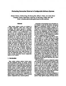
Figure 6 provides the runtimes (in seconds) of analyzing variants of the safety property for different values of maxStep, one per trace. In order to reduce stochastic noise, we provide runtimes averaged over 10 independent analyses. The figure provides two kinds of scalability analysis: (1) by focusing on a single trace we can fix the number of

1 2 3 4 5 6

13

40 Until 50000 steps Until 40000 steps Until 30000 steps Until 20000 steps Until 10000 steps

Analysis runtime (s)

35 30 25 20 15 10 5 0 5

10

15

20 25 Floors in the model

30

35

40

Fig. 6. Runtime in seconds for the analysis of Listing 13; each trace refers to variants of the property for maxStep in {10, 20, 30, 40, 50}×103

performed simulation steps, and vary the size of the system (the floors); (2) by considering one point of the x-axis (the floors), we can fix the model under analysis, and vary the number of performed simulation steps. In both cases, we note a linear increase in the obtained runtime. All experiments were performed on a static pre-defined configuration consisting of all features except Park. 6.2

Safe lock

To illustrate the flexibility of our approach to model case studies from different application domains, we show in this section how QFLan can be used to perform risk assessment in security scenarios with high variability. In particular, we focus on the use of attack trees and the seminal example from that area, namely the Safe Lock [59]. Fig. 7(a) presents the original attack tree from [59]. It provides a specification of a risk assessment for a safe lock system. An attack tree is essentially an and/or tree, where nodes represent goals, and sub-trees represent sub-goals. In this case, the root node represents the main threat being analyzed, namely the lock being opened by an attacker. Each of its four children are possible ways of enacting such a threat. The sub-goal Eavesdrop has two sub-goals that need to be accomplished (thus their combination as and-children). Nodes are decorated with an estimation of the cost that the attacker would have to pay to succeed in enacting the corresponding action. The classical analysis of such trees is to compute the minimal cost for an attacker to succeed. Attack trees can easily be modelled as feature diagrams, with the following rationale: a node, which in an attack tree represents a goal, can be modeled as a feature of the system, that the attacker tries to activate. The sub-goal relation is modeled by the feature hierarchy. In particular, the attack tree of our case study can be modeled as in Fig. 7(b). We introduce a slight variation to overcome a well-known limitation of the original attack trees, namely the inability to encode the ordering of events. Indeed, Listen to Conversation should occur before Get Target to State Combo, which we can model with a requires cross-tree constraint. As a matter of fact, the flexibility of the way feature models are specified in QFL AN allows us to specify richer relations among sub-goals. For instance, we can specify that

Eavesdrop is only successful if the attacker first listens to a conversation and then gets the target to state the combo, thus refining the original and-relation among such subgoals. This is similar in spirit to the extension of attack trees with sequential conjunction from [60], which imposes orders on the execution of actions in the tree. Further constraints can be imposed on execution, in line with those discussed for the other examples. A noteworthy advantage of modeling such scenarios with QFL AN is that we can model the behavior of several classes of attackers and study their performance, and thus the robustness of the system against them. To exemplify this, we have considered two attackers, sketched in Fig. 8. Their full process specifications can be found in Listing 14. install(PickLock)

1

install(PickLock) ··· install(Bribe)



IDLE

TRY P ICK L OCK

try

Q o

.. .

fail

IDLE

try

.

TRY B RIBE

install(Bribe)

Fig. 8. Behavior of PowerfulAttacker (left) and FailingAttacker (right)

The Powerful attacker always succeeds when trying to achieve a goal and has unlimited resources. Instead, the Failing attacker can fail to successfully achieve a goal and may need several attempts to achieve them. This is modeled using rates. In addition, (s)he has limited resources. begin p r o c e s s e s diagram begin p r o c e s s powerfulAttacker s t a t e s = idle transitions = idle -( i n s t a l l (PickLock) , 1 )-> idle , idle -( i n s t a l l (CutOpenSafe) , 1 )-> idle , idle -( i n s t a l l (InstallImproperly) , 1 )-> idle , idle -( i n s t a l l (FindWrittenCombo) , 1 )-> idle , idle -( i n s t a l l (Threaten) , 1 )-> idle , idle -( i n s t a l l (Blackmail) , 1 )-> idle , idle -( i n s t a l l (ListenToConversation) , 1 )-> idle , idle -( i n s t a l l (GetTargetToStateCombo) , 1 )-> idle , idle -( i n s t a l l (Bribe) , 1 )-> idle end p r o c e s s begin p r o c e s s failingAttacker s t a t e s = idle , tryPickLock , tryCutOpenSafe , tryInstallImproperly , tryFindWrittenCombo , tryThreaten , tryBlackmail , tryListenToConversation , tryGetTargetToStateCombo , tryBribe transitions = // Try an attack idle -( try , 1 , {cumul_cost = cumul_cost + 1} )-> tryPickLock , idle -( try , 1 , {cumul_cost = cumul_cost + 1} )-> tryCutOpenSafe , idle -( try , 1 , {cumul_cost = cumul_cost + 1} )-> tryInstallImproperly , idle -( try , 1 , {cumul_cost = cumul_cost + 1} )-> tryFindWrittenCombo , idle -( try , 1 , {cumul_cost = cumul_cost + 1} )-> tryThreaten , idle -( try , 1 , {cumul_cost = cumul_cost + 1} )-> tryBlackmail , idle -( try , 1 , {cumul_cost = cumul_cost + 1} )-> tryListenToConversation , idle -( try , 1 , {cumul_cost = cumul_cost + 1} )-> tryGetTargetToStateCombo , idle -( try , 1 , {cumul_cost = cumul_cost + 1} )-> tryBribe , // Successful attack tryPickLock -( i n s t a l l (PickLock) , 1 )-> idle , tryCutOpenSafe -( i n s t a l l (CutOpenSafe) , 1 )-> idle , tryInstallImproperly -( i n s t a l l (InstallImproperly) , 1 )-> idle , tryFindWrittenCombo -( i n s t a l l (FindWrittenCombo) , 1 )-> idle , tryThreaten -( i n s t a l l (Threaten) , 1 )-> idle , tryBlackmail -( i n s t a l l (Blackmail) , 1 )-> idle , tryListenToConversation -( i n s t a l l (ListenToConversation) , 1 )-> idle , tryGetTargetToStateCombo -( i n s t a l l (GetTargetToStateCombo) , 1 )-> idle , tryBribe -( i n s t a l l (Bribe) , 1 )-> idle , // Failed attack tryPickLock -( fail , 10 )-> idle , tryCutOpenSafe -( fail , 10 )-> idle , tryInstallImproperly -( fail , 10 )-> idle , tryFindWrittenCombo -( fail , 10 )-> idle , tryThreaten -( fail , 10 )-> idle , tryBlackmail -( fail , 10 )-> idle , tryListenToConversation -( fail , 10 )-> idle , tryGetTargetToStateCombo -( fail , 10 )-> idle , tryBribe -( fail , 10 )-> idle end p r o c e s s end p r o c e s s e s diagram

Listing 14. Two kind of attackers for the safe lock scenario

Clearly, any reasonable attacker should stop attacking once an attack has been successful. This can be naturally ex-

1 2 3 4 5 6 7 8 9 10 11 12 13 14 15 16 17 18 19 20 21 22 23 24 25 26 27 28 29 30 31 32 33 34 35 36 37 38 39 40 41 42 43 44 45 46 47 48 49 50

14

(a) Schneier’s simple attack tree against a physical safe

(b) An attributed feature model representing the attack tree

Fig. 7. Attack tree: (a) redrawn from [59]; (b) feature model representation of it

pressed in QFL AN using the action constraints in Listing 15, which block the attacker after an attack succeeded. 1 2 3 4

begin a c t i o n c o n s t r a i n t s do(tryAction) -> !has(OpenSafe) do( i n s t a l l (...)) -> !has(OpenSafe) end a c t i o n c o n s t r a i n t s

Listing 15. Constraints to stop attacks after success

QFL AN’s rich specification language allows to express, e.g., further constraints on the accepted classes of attacks. Consider for instance the two constraints in Listing 16. In the first one, we restrict to (successful) attacks that cost less than 100 units (i.e. that install features with less than that price). Instead, the second constraint restricts to attack attempts (independently of their success) that cost less than 10 units. Noteworthy, using the first constraint we restrict the family of admissible products, while the latter constraint regards only the behavioral part of the model. 1 2 3 4 5 6 7

begin q u a n t i t a t i v e c o n s t r a i n t s // Restrict to attacks that cost less than 100 { cost(Root)