Interaction Testing of Highly-Configurable Systems in the ... - UNL CSE

Interaction Testing of Highly-Configurable Systems in the Presence of Constraints Myra B. Cohen, Matthew B. Dwyer, Jiangfan Shi Department of Computer Science and Engineering University of Nebraska - Lincoln Lincoln, Nebraska {myra,

dwyer, jfshi}@cse.unl.edu

ABSTRACT Combinatorial interaction testing (CIT) is a method to sample configurations of a software system systematically for testing. Many algorithms have been developed that create CIT samples, however few have considered the practical concerns that arise when adding constraints between combinations of options. In this paper, we survey constraint handling techniques in existing algorithms and discuss the challenges that they present. We examine two highlyconfigurable software systems to quantify the nature of constraints in real systems. We then present a general constraint representation and solving technique that can be integrated with existing CIT algorithms and compare two constraint-enhanced algorithm implementations with existing CIT tools to demonstrate feasibility.

Categories and Subject Descriptors D.2.5 [Software Engineering]: Testing and Debugging

General Terms Algorithms,Verification

Keywords Combinatorial interaction testing,constraints,covering arrays,SAT

1.

INTRODUCTION

Software development is, increasingly, shifting from the production of individual programs to the production of families of related programs [26]. This eases the design and implementation of multiple software systems that share a common core set of capabilities, but have key differences, such as the hardware platform they require, the interfaces they expose, or the optional capabilities they provide to users. Often times significant reuse can be achieved by implementing a set of these systems as one integrated highly-configurable software system. Configuration is the process of binding the optional features of a system to realizations in order to produce a specific software system, i.e., a member of the family. The concept of a highly-configurable software system arises in many different settings differentiated by the point in the development process when feature binding occurs, i.e., the binding time. Permission to make digital or hard copies of all or part of this work for personal or classroom use is granted without fee provided that copies are not made or distributed for profit or commercial advantage and that copies bear this notice and the full citation on the first page. To copy otherwise, to republish, to post on servers or to redistribute to lists, requires prior specific permission and/or a fee. ISSTA’07, July 9–12, 2007, London, England, United Kingdom. Copyright 2007 ACM 978-1-59593-734-6/07/0007 ...$5.00.

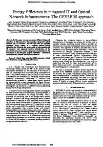
An example of very early feature binding is seen in software product lines. A software product line (SPL) uses an architectural model to define a family of products built from a core set of platforms and customized through the identification of points of variability and commonality. Variability points allow the developer to plug in different variations of a feature (variant) while still maintaining the overall system architecture. At the other end of the spectrum are dynamically reconfigurable systems, where feature binding happens at run-time and may, in fact, happen repeatedly. NASA’s Deep Space 1 software is an example of such a system that uses online planning to activate and deactivate modules in the system based on spacecraft and mission status [11]. In between are the common class of user configurable systems. These are programs such as desktop applications, web servers, or databases, that allow users to modify a set of pre-defined options, e.g., command-line parameters or configuration file settings, as they see fit and then run the program with those options. Highly-configurable systems present significant challenges for validation. The problem of testing a single software system has been replaced with the much harder problem of testing the set of software systems that can be produced by all of the different possible bindings of optional features. A single test case may run without failing under one configuration, however the same test case may fail under a different one [19, 32]. One cause for this is the unintended interaction of two more bindings for features. Figure 1 presents a simplified mobile phone product line that we use to illustrate the challenges of testing highly-configurable software; the challenges are present in systems with later binding times as well. This product line is hypothetical, but its structure is reflective of portions of the Nokia 6000 series phones [24]. The product line supports three display options (16MC, 8MC, BW) and can have either a text email viewer (TV), graphical email viewer (GV) or no viewer (NOV). A phone may be built with two types of camera (2MP or 1MP) or without a camera (NOC), with a video camera (VC) or without a video camera, and with support for video ringtones (VR) or without that support. There are a total of 108, (3 × 3 × 3 × 2 × 2), different phones that can be produced by instantiating this software product line. For each one, we will need to run a test suite if we wish to fully test the family of products. When we run test suites, they may behave differently when different features are present. For instance a problem with the email viewer may not appear under the 8MC display, but may only appear with 16MC. Similarly a problem in the 16MC display may only appear with a VC. Since testing the complete set of product line instances is most likely infeasible, testing techniques that sample that set can be used to find interaction faults. This is commonly called combinatorial interaction testing (CIT) [4] and a primary approach to such testing is to systematically sample the set of instances in

Product Line Options (factors) Possible Values

Display 16 Million Colors 16MC

8 Million Colors 8MC

Black and White BW

Email Viewer Graphical

Camera 2 Megapixels

GV

Text

2MP

1 Megapixel

TV

1MP

None

None

NOV

NOC

Video Camera

Video Ringtones

Yes

Yes

VC

VR

No

No

!VC

!VR

Constraints on Valid Configurations: __________________________________________________________________________________________________

(1) Graphical email viewer requires color display (2) 2 Megapixel camera requires a color display (3) Graphical email viewer not supported with the 2 Megapixel camera (4) 8 Million color display does not support a 2 Megapixel camera (5) Video camera requires a camera and a color display (6) Video ringtones cannot occur with No video camera (7) The combination of 16 Million colors, Text and 2 Megapixel camera will not be supported

Figure 1: Mobile phone product line such a way that all t-way combinations of features are included; pairwise or 2-way combinations are the most commonly studied. A significant literature exists that describes foundational concepts, algorithms, tools, and experience applying interaction testing tools to real systems. One prime objective of this body of work is to produce the smallest subset of configurations for a system that achieves the desired t-way coverage. At the bottom of Figure 1, we list seven constraints that have been placed on the valid product instances which can be created. Constraints like these were common in the Nokia 6000 series. They may be due to any number of reasons, for example, inconsistencies between certain hardware components, limitations due to available memory and software size, or simply marketing decisions. We present natural language representations of constraints since that is how they are typically described in software documentation. Taken together these constraints reduce the number of product instances to 31, but rather than simplifying the interaction testing problem they actually make it much more challenging. As explained in Section 2, existing algorithms and tools for combinatorial interaction testing either: 1. ignore constraints all together; 2. require the user to explicitly define all illegal configurations; 3. attempt to bias test generation to avoid constraints “if possible”, but don’t guarantee the avoidance of illegal configurations; 4. mention constraints as a straightforward engineering extension to be solved later; or 5. use a proprietary (unpublished) method that cannot be leveraged by the research community. This is problematic for multiple reasons. Ignoring constraints may lead to the generation of test configurations that are illegal and this can lead to inaccurate test planning and wasted effort. Even a small number of constraints can give rise to enormous numbers of illegal configurations, as we illustrate in Section 4, and asking a user to produce those is both excessively time consuming and highly error-prone. As we explain in Section 3.2, biasing strategies will not work in the relatively common situation where multiple constraints interact to produce additional implicit constraints. In this paper, we make several contributions: (i) we explain the variety and type of constraints that can arise in highly-configurable systems and report on the constraints found in two non-trivial software systems – SPIN [17] and GCC [12], (ii) we present a technique for compiling constraints into a boolean satisfiability (SAT)

problem and integrating constraint checking into existing algorithms, and (iii) we report our experiences integrating this technique into both greedy and simulated annealing algorithms for interaction test generation and on the cost and effectiveness of the resulting CIT techniques. Our primary goals are to expose the magnitude and subtlety of constraints found in realistic configurable systems and to provide an open and comprehensive description of techniques for handling these; we believe it is the first in the interaction testing literature. Although we prototype our technique on two specific algorithms, we expect that it can be generalized to work with others. This work is just the first step towards widely applicable cost-effective interaction testing for large-scale highly-configurable systems, but it is an essential step. The rest of this paper is organized as follows. In the next section, we provide some background on interaction testing and existing algorithmic techniques. We then discuss various types of constraints and show the implications for various algorithms that are used today. Section 4 presents a case study of two real configurable software systems to show the extent to which constraints exist. Section 5 presents our solution for incorporating constraints into two types of algorithms for constructing constrained covering arrays. Section 6 validates our techniques on a set of examples and compares them with some known algorithms. Finally in section 7 we conclude and present our future work.

2.

BACKGROUND

In the example in Figure 1, the mobile phone software product line contains a total of 108 possible product line instances before incorporating system constraints. The number of possible instances of a product line grows exponentially in relation to the number of factors. If there are 4 factors each with 5 possible values, there are 54 possible product instantiations. Developers may wish to generate a set of configurations to perform testing of the whole product line. Testing all possible instances of the product line, however, is usually intractable; therefore as a validation method this will not scale. One sampling method that has been used to systematically sample and test instances of software for other types of configurable systems is to sample all pairs or t-way combinations of options [4]. We will call this CIT sampling. Figure 2 is an example of a pairwise or 2-way CIT sample for the phone SPL. We are ignoring the constraints that are listed, but will return to them in the following sections. In this example we have a set of configurations (a product instance that has one value selected for each factor) that combine all pairs of values between any two of the factors. For instance all displays are combined with both of the email viewers as well as without any email viewer. Likewise, all email viewers have been tested with all camera options, as well as with all video camera options and with and without video ringtones. Many studies have shown that CIT is a powerful sampling technique for functional input testing, that may increase the ability to find certain types of faults efficiently [1, 4, 22] and that it provides good code coverage [4, 10]. Recent work on CIT has studied its use on both user configurable systems [19, 32], and on software product lines [7, 23]. One of the main focuses in the literature on interaction testing has been on developing new algorithms to find smaller t-way samples [5, 13, 14, 15, 29, 31]. However, much of this literature largely ignores the practical aspects of applying CIT to real systems, which limits the effectiveness of this work. In this paper we focus on one difficult, yet prevalent issue which may confound existing algorithms; that of handling constraints.

Display

Email Viewer

Camera

Video Camera

Video Ringtones

1

16 Million Colors

None

1 Megapixel

Yes

Yes

2

8 Million Colors

Text

None

No

No

3

16 Million Colors

Text

2 Megapixels

No

Yes

4

Black and White

None

None

No

Yes

5

8 Million Colors

None

2 Megapixels

Yes

No

6

16 Million Colors

Graphical

None

Yes

No

7

Black and White

Text

1 Megapixel

Yes

No

8

8 Million Colors

Graphical

1 Megapixel

No

Yes

9

Black and White

Graphical

2 Megapixels

Yes

Yes

Figure 2: Pairwise CIT sample ignoring constraints

2.1

CIT Samples: Covering Arrays

Before we discuss the various techniques for constructing CIT samples we begin with some definitions. A t-way CIT sample is a mathematical structure, called a covering array. D EFINITION 2.1. A covering array, CA(N ; t, k, v), is an N × k array on v symbols with the property that every N × t sub-array contains all ordered subsets of size t from the v symbols at least once. D EFINITION 2.2. A special instance of this problem is an orthogonal array, OA(t, k, v) where every ordered subset occurs exactly once. In this case N is not used because the exact size of the array is always v t . The strength of a covering array is t, i.e. this defines 2-way, 3-way sampling. The k columns of this array are called factors, where each factor has v values. Although the trivial mathematical lowest bound for a covering array is v t , this is often not achievable and sometimes the real bound is unknown [14]. As can be seen in our phone example, most software systems do not have the same number of values for each factor, i.e. we don’t have a single v. A more general structure can be defined called a mixed level covering array. D EFINITION 2.3. A mixed level covering array, M CA(N ; t, k, (v1 , v2 , ..., vk )), Pk is an N × k array on v symbols, where v = i=1 vi , with the following properties: (1) Each column i (1 ≤ i ≤ k) contains only elements from a set Si of size vi . (2) The rows of each N × t sub-array cover all t-tuples of values from the t columns at least one time. We use a shorthand notation to describe mixed level covering arrays by combining equal entries in (vi : i ≤ 1 ≤ k). For example three entries each equal to 2 can be written as 23 . Figure 2 illustrates a 2-way CIT sample, M CA(9; 2, 33 22 ), for the phone example. In this paper when we use the term covering array we will use it to mean both types of arrays.

2.2

Finding CIT Samples

Finding a covering array for a configurable system is an optimization problem where the goal is to find a minimal set of configurations that satisfy the coverage criteria of all t-sets. Many algorithms and tools exist that construct covering arrays. We discuss three general classes next. Mathematical (or algebraic) constructions: When certain parameter combinations of t, k, v for are met, mathematical tech-

niques (both direct and recursive) can be used to construct covering arrays [13, 14]. Although constructions are fast and produce small covering arrays efficiently, they are not general. TConfig [31], Combinatorial Test Services (CTS) [13] and TestCover [27] all use constructions to generate covering arrays. Greedy algorithms: There are two classes of greedy algorithms that have been used to construct covering arrays. The majority are the one-row-at-a-time variation of the automatic efficient test case generator (AETG)[4].We call these AETG-like. We summarize the generic framework for these types of algorithms (for more detail see [3]). A single row for the array is constructed at each step until all t-sets have been covered. For each row, a set of M candidates are built in parallel. The choice in the size of M is one of the differentiators of these algorithms. The best candidate row is then selected. To build a single row, the factors are ordered based on the algorithm’s heuristics. Then each value of that factor is compared with all of the values already selected and fixed. The one that produces the most new t-sets is chosen. Some existing algorithms that fit into this category are the Test Case Generator [30], the Deterministic Density Algorithm (DDA) [8] and PICT [9]. The second type of greedy algorithm is the In Parameter Order (IPO) algorithm [29]. It begins by generating all t-sets for the first t factors and then incrementally expands the solution, both horizontally and vertically using heuristics until the array is complete. Meta-heuristic Search: Several examples of meta-heuristic search have appeared in the literature such as simulated annealing, genetic algorithms and tabu search [5, 25]. We will use simulated annealing as is described in [5] as an example. In simulated annealing an N × k array is randomly filled with legal values. Then a series of transformations take place that bring the solution closer and closer to a covering array. The transformation is a move method. In this method, a single location in the array is chosen and a new value replaces the old. If the solution covers the same number or more t-sets (is fitter), then the new solution is kept and a move is made. Worse moves are allowed with a small probability determined by the annealing parameters (the cooling schedule). Since N is not known at the start, a binary search is used. Multiple runs of annealing occurs, after which a smaller or larger N is tried based on the success of the current run. Termination criteria allow the algorithm to stop and fail after a period of time.

2.3

Existing Constraint Support

Many of the algorithmic techniques provide extensions to handle certain practical aspects of real software, such as seeded sets of configurations, but solutions for handling constraints are less than satisfactory. There has been relatively little discussion in the literature of how to construct a covering array in the presence of constraints such as those seen in the bottom of Figure 1. There are seven constraints that will cause invalid configurations in the covering array. In Figure 2 these are highlighted. To satisfy the constraints, the highlighted configurations must be removed and others added back to fulfill t-way criteria. Bryce and Colbourn state that asking if a configuration exists satisfying a set of given constraints is an NP hard problem [2]. They also argue that there is a strong need for a workable solution. Although some existing tools will handle constraints, we have found that most solutions are lacking in one of several aspects. We believe there should be an open, general solution, that can be applied to existing algorithms. Given the extent and variety of research on CIT algorithms, it seems unsatisfactory to create an orthogonal algorithm just to handle constraints. Instead we see constraints as an extension that is cross-cutting. We have categorized the constraint handling in a variety of the algorithms/tools for constructing covering arrays and summarized

Algorithm/Tool AETG DDA Whitch:CTS Whitch:TOFU IPO TestCover Simulated Annealing PICT Constraint Solver

Citation [4] [2, 8] [13] [18] [29] [27] [6] [9] [15]

Tool Category AETG-Like Greedy AETG-Like Greedy Construction;AETG-Like Greedy Unknown Other Greedy Construction Meta-Heuristic Search AETG-Like Greedy Constraint solving

Constraint Handling

Re-Implementable

REMODEL

PARTIAL

SOFT ONLY

YES

SIMPLE ; EXPAND

NO

EXPAND

NO

NONE

−−

REMODEL

NO

SOFT ONLY

YES

FULL

PARTIAL

NONE

−−

Table 1: Summary of constraint handling in existing algorithms/tools these in Table 1. We restrict our discussion to constraints that involve illegal combinations of two or more factor-values, since this is the most common scenario discussed. We classify the constraint handling technique, as REMODEL, EXPAND, SOFT , SIMPLE, NONE or FULL.We will discuss each of these in turn. For each tool, we state whether we believe it is re-implementable or not. We attempt to capture the amount of information that is available to researchers who may want to implement these algorithms on their own. In this category NO means that the method is a proprietary commercial product, no research papers have been published to our knowledge on this topic, or a paper exists but it does not provide enough information for us to determine how constraints are actually implemented. PARTIAL means that some information about constraint handling has been provided, but we do not believe it is enough to re-implement the technique fully. Finally, YES means that we believe the technique can be re-implemented by someone with a technical background in CIT algorithms. REMODEL: Some algorithms require the user to re-model their input into separate unconstrained inputs to be combined at the end of processing. This is the main approach that AETG takes [4]. Small examples have been provided and in [4, 20] some insight into the idea of implicit constraints (see Section 3.2) is given. The authors suggest that AETG handles more than re-modeling but there is no direct explanation of how this is done. We place AETG into the PARTIAL category. The TestCover service [27] uses direct product block notation to identify a set of allowed test cases computed as a direct product of compatible factor values. It takes a collection of these products as input data to define the set of all allowed test cases, implicitly defining the constraints [28]. This requires the user, in essence, to re-model their input. Since it is a commercial product we do not know how constraints are incorporated. EXPAND: Some tools expose implicit constraints (see Section 3.2) by requiring the user to expand the input. One such tool is the Intelligent Test Case Generator (Whitch) by IBM [18] that includes two algorithms for finding covering arrays, TOFU, and Combinatorial Test Services(CTS) [13]. The interface for both algorithms requires that forbidden combinations are expressed as all possible forbidden configurations. In the phone example, the first constraint states that GV cannot occur with BW. In Whitch an enumeration of all configurations containing GV and BW would be required. There are twelve such configurations in this example. As the number of factors and values grows, this may explode. If we have 20 factors with 5 values each, then this single constraint would require that 518 configurations be listed. In the literature, CTS proposes to support simple constraints so we include it in this category as well. Neither TOFU or CTS provides details of about how they implement constraint handling. SOFT ONLY: The deterministic density algorithm, (DDA) [8] is an AETG-like algorithm. In [2] the authors extend DDA to in-

clude constraint handling by weighting tuples as desirable or not. They use this method to avoid tuples if possible. They term these SOFT CONSTRAINTS . Although they provide a discussion of HARD CONSTRAINTS their algorithm does not handle these. Instead, they state that this is “a constraint satisfaction problem” and out of the domain of their algorithm. As we highlight in in the next section, their algorithm will always contain forbidden t-sets under certain circumstances. In their experimentation with random constraints these occurred around 3% of the time. In [6], simulated annealing was augmented with an initialization phase that allowed the specification of t-sets that do not need to be covered. Although the purpose of this was not constraint handling, this mechanism can be used for soft constraints as in Bryce and Colbourn. No weighting scheme is used, so the avoidance mechanism is not as strong. Both algorithms only consider constraints of size t although there may be ones of higher or lower arity. Both algorithms are re-implementable given some algorithmic background in CIT. FULL: We use the term FULL when the tool appears to handle constraints of any arity and does not require the user to expand or remodel the input. PICT is a Microsoft internal tool, developed by Czerwonka [9]. It uses an AETG-like algorithm optimized for speed. Specifically, it uses M = 1 and skips the parallel aspect of AETG. In [9] a discussion of the algorithm and constraint handling says that as they build their solutions they check to see if the solution is legal, but this gives us little detail about how this check is actually implemented. They provide some insight into the transitive nature of some constraints but do not expose enough details for re-implementation. We classify this as PARTIAL. NONE: The last two algorithms, IPO [29] and Hnich et al. [15] contain no support for constraint handling. Hnich et al. use constraint solving to build covering arrays by translating the definition into a Boolean satisfiability problem. They use a SAT solver to generate their solution. In their paper, they term our type of constraint as side constraints and leave this as future work. We highlight their algorithm because we use some of their ideas to implement our algorithmic extensions. Given this brief survey of constraint handling in the literature, it seems that there is no general solution that will scale to a large number of factors and values, while keeping the burden of manipulating constraints off of the software tester. It is a topic that is mentioned often, but one that has been largely ignored. Due to the complexity that even simple constraints add to the CIT sampling technique, this is not surprising. The next section discusses some of reasons this problem is hard, and provides insight into why no solution has yet been proposed.

3.

IMPACT OF CONSTRAINTS ON CIT

We illustrate concepts related to constraints and their impact on interaction testing through the example in Figure 1. For this prod-

Display

Email Viewer

Camera

Video Camera

Video Ringtones

1

16 Million Colors

None

2 Megapixels

No

No

2

16 Million Colors

Graphical

1 Megapixel

No

No

3

8 Million Colors

None

1 Megapixel

Yes

4

16 Million Colors

Graphical

None

5

16 Million Colors

Text

6

Black and White

7

Display

Email Viewer

Camera

Video Camera

Video Ringtones

1

16 Million Colors

None

1 Megapixel

Yes

Yes

2

8 Million Colors

Text

None

No

No

Yes

3

16 Million Colors

Text

2 Megapixels

No

Yes

Yes

Yes

4

Black and White

None

None

No

Yes

1 Megapixel

Yes

No

5

8 Million Colors

None

2 Megapixels

Yes

No

None

1 Megapixel

Yes

Yes

6

16 Million Colors

Graphical

None

Yes

No

8 Million Colors

Graphical

2 Megapixels

Yes

Yes

7

Black and White

Text

1 Megapixel

Yes

No

8

Black and White

Text

2 Megapixels

No

Yes

8

8 Million Colors

Graphical

1 Megapixel

No

Yes

9

8 Million Colors

Text

None

No

No

9

Black and White

Graphical

2 Megapixels

Yes

Yes

10

Black and White

None

None

No

No

Constraints: __________________________________________________________________________________________________

(1) Graphical email viewer requires color display (2) 2 Megapixel Camera requires color display (3) Graphical email viewer not supported with the 2 Megapixel camera

Constraints: __________________________________________________________________________________________________

(1) Graphical email viewer requires color display

Figure 3: A single constraint can increase sample size No

Forbidden Tuples

Derived from

1

(Black and white display, Graphical email viewer)

1

2

(Black and white display, 2 Megapixel camera)

2

3

(Graphical email viewer, 2 Megapixel camera)

3

4

(8 Million color display, 2 Megapixel camera)

4

5

(Video camera=Yes, Camera=No)

5

6

(Video camera=Yes, Black and white display)

5

7

(Video ringtones= Yes, Video camera=No)

6

8

(16 Million colors, Plain text, 2 Megapixel camera)

7

Figure 4: Mapping constraints to forbidden tuples uct line there are seven constraints on the feasible configurations. These constraints could be expressed in a number of different forms and styles; we show constraints using several different phrasings including: requires, not supported and cannot occur. Constraints may relate differing numbers of configuration choices; we show constraints between pairs and triples of option choices. It is important to emphasize that constraints that are expressed explicitly in the description of a configurable system can give rise to implicit relationships among option choices. In fact, treatment of these implicit relationships is the key complicating factor in solving constrained CIT problems. In this paper, we encode all constraints in the canonical form of forbidden tuples which define combinations of factor-value pairs that cannot occur in a feasible system configuration; tuples can vary in their arity. Figure 4 illustrates the forbidden tuples for the constraints in the example; note that a single constraint may give rise to multiple forbidden tuples depending on the nature of the constraint and the size of factor-value domains. It is important to note that other choices are possible for encoding constraints, e.g., we could express that when factor f has value v in a configuration then factor g must have value w as f = v ⇒ g = w. The question of what representation is most succinct or computationally tractable for a given constrained MCA is open. Other researchers have discussed similar concepts to forbidden tuples. Forbidden configurations [13] are configurations of features that are not allowed either because they cannot be combined for

Figure 5: Constraints can remove configurations some structural reason, or because the designers of the system have decided these will never be instantiated; forbidden tuples can be thought of as partial forbidden configurations. Bryce and Colbourn [3] differentiate between forbidden combinations and combinations that should be avoided but may legally be present in a system configuration. Figure 4 shows seven 2-way and one 3-way forbidden tuples for this product line. It is clear that constraints will reduce the number of feasible configurations for a system; in the example, the number is reduced from 108 to 31. The impact on interaction testing is more subtle since its goal is to cover all t-way combinations and not the set of feasible configurations. In the example, the 8 forbidden tuples reduce the number of pairs needed to satisfy a 2-way cover from 67 pairs to 57 pairs. Due to the nature of the constraints, however, those 57 cannot be packed into a smaller set of configurations than could the original 67. The result is that the size of the CIT sample for this problem is the same, regardless of constraints. The impact of constraints will, of course, vary with the problem, but their presence causes problems for many existing CIT tools. This is due to the fact that many of the existing algorithms and construction techniques used in these tools are based on the mathematical theory of covering arrays. In the presence of constraints that theory does not apply, in general. More specifically, in the presence of constraints: 1. the number of required t-sets to produce a solution cannot be calculated from the MCA parameters, 2. lower (upper) bounds on the size of a solution cannot be calculated, and 3. mathematical constructions cannot be directly applied without non-trivial post-processing to remove infeasible configurations, and add back new configurations to satisfy required coverage. In general, calculating properties of CIT solutions becomes extremely difficult due to the irregularity introduced by constraints. In fact, it is even difficult to tell whether a set of constraints is internally consistent in the context of a configurability model; if it is not then there may be no feasible configurations.

3.1

Impact on Sample Size

Adding constraints always reduces the number of feasible system configurations, but it is not guaranteed to reduce the size of the CIT sample needed to achieve a desired t-way coverage. The impact on sample size results from the interaction of the number and type of constraints and the model itself. We illustrate both increased and decreased sample sizes relative to the 2-way covering array sample for the example SPL shown in Figure 2, which has 9 configurations. Increasing the Sample Size: The first three columns of Figure 2 constitute a special type of a covering array, an orthogonal array. Orthogonal arrays only exist for certain combinations of parameters of t, k, v [14]. In this structure each pair occurs exactly one time, instead of at least one time. Many tools, such as the commercial AETG, CTS and TestCover, will use mathematical constructions to build orthogonal arrays when the covering array parameters indicate that this is possible. These constructions do not take into account constraints. Adding a single constraint may increase the sample size required for satisfying 2-way coverage. Consider the first forbidden tuple from table 4, (BW,GV). Configuration 9 in Figure 2 includes this tuple and must be eliminated. That configuration also includes pairs that are not forbidden and not included in any other configuration, e.g., (GV, 2MP). To produce a CIT sample, we must add additional configurations to include those pairs. Adding such a configuration will, however, force us to repeat pairs in previous configurations. For instance, we must combine GV with either of the color displays thereby repeating a pair from either configuration 6 or 8. Because of the interaction between choices made in other configurations and the constraints for this problem at least 10 configurations are now needed for 2-way coverage; a solution is shown in Figure 3. The lower bound for the original unconstrained covering array is no longer valid, and furthermore the orthogonal nature of this solution structure has been broken, i.e., there are now repeated pairs (see shading in Figure 3). Implications: Tools that rely on upper bounds on achievable solution sizes may not work. Tools that use mathematical constructions must post-process their results to remove infeasible configurations and add configurations to recover lost coverage. Reducing the Sample Size: Adding certain sets of constraints may reduce the size of a covering array solution. If, for instance, we add constraints (1-3) from Figure 4 to the SPL model, we can remove an entire 3-tuple from the first three columns of our table (BW, GVV, 2MP). Figure 5 shows a solution with only 8 configurations. Implications: Tools that rely on the existence of lower bounds on achievable sample sizes may not work in the presence of constraints. Tools that use mathematical constructions will need to post-process their results to remove rows to achieve optimal results.

3.2

Implied Forbidden t-sets

Consider a CIT problem that is targeting t-way coverage. Each forbidden tuple of arity t trivially implies a t-way combination that cannot be present anywhere in the CIT sample. More generally, the conjunction of a set of forbidden tuples of varying arity imply a number of t-sets none of which can be present in the CIT sample. These forbidden t-sets may not be obvious to the person modeling a highly-configurable system [20]. Consider constraints (4-5) from Figure 1. These constraints are encoded as forbidden pairs (46) in Figure 4. We write forbidden tuples as logical formula of the form: ¬(P ∧Q), where P and Q are atomic propositions indicating the presence of the configuration choices abbreviated in Figure 1. The three forbidden pairs are: ¬(V C ∧ N OC), ¬(V C ∧ BW ),

and ¬(V R ∧ ¬V C), and it is not difficult to prove that: ¬(V C ∧ N OC) ∧ ¬(V C ∧ BW ) ∧ ¬(V R ∧ ¬V C) ⇒ ¬(V R ∧ BW )

but determining the set of implied forbidden t-sets or even the size of that set is computationally demanding. Determining forbidden t-sets by hand would be infeasible for all but the smallest problems, e.g., due to the combinatorial nature of the candidate t-sets and the difficulty in identifying dependent combinations of constraints – the first conjunct in the above implication is unnecessary for the proof. Implications: Many existing CIT algorithms rely on calculating the number of uncovered t-sets during the calculation of the sample; they continue until this number is zero. The presence of constraints makes it impossible to calculate the number of uncovered t-sets from MCA parameters. This has a significant impact on greedy algorithms and simulating annealing approaches that we address in Section 5. For example, the discussion in Bryce et al. [2] that proposes to bias the sample to “avoid” certain t-sets, actually guarantees that it will always include some forbidden tuples in the presence of implied forbidden t-sets. Otherwise their algorithm will never terminate. Tools such as Whitch force the user to list all forbidden t-sets which we believe to be infeasible for non-trivial problems with implied forbidden t-sets; the case studies in Section 4 clearly indicate this. Implied forbidden t-sets from low-order tuples: The arity of a forbidden tuple may or may not be t. When forbidden tuples of arity < t are present the number of implied forbidden t-sets will, in general, be exponential in the number of factors. For example, a system with 5 binary configuration options, o1 , . . . , o5 and a single forbidden pair (o1 , o2 ) can be embedded in 6 different 3-way sets and 12 different 4-way sets. These sets must be forbidden when calculating 3-way or 4-way CIT samples. Implications: Exponentially many implied forbidden t-sets may arise in the presence of low-order constraints. Implied forbidden t-sets from high-order tuples: Forbidden tuples with arity greater than t do not typically pose the same problem. This is because a forbidden tuple does not forbid the tuples embedded within it. Consequently, they do not need to be forbidden as t-sets from a CIT sample. The combinations of higher-order tuples must still be considered because it is possible for implicit forbidden t-sets to arise. In Figure 6, the third constraint is implied in part by the 3-way constraint from Figure 4. Implications: Algorithms which use weighting of t-sets or rely on already covered t-sets to construct solutions, may suffer since higher arity forbidden tuples provide little guidance. This may negatively impact the quality of solutions (i.e. they may get large) or the performance may suffer (long run-times may be encountered).

3.3

Constrained Covering Arrays

The presence of constraints demands a new definition for a proper CIT sample. Integral to this definition is the concept of whether a t-set is consistent with a set of constraints. D EFINITION 3.1. Given a set of constraints C, a given t-set, s, is C-consistent if s is not forbidden by any combination of constraints in C. This definition permits flexibility in defining the nature of constraints and how they combine to forbid combinations; in Section 5, we define F -consistency for constraints encoded as a set of forbidden tuples. We provide a definition of constrained covering arrays that is parameterized by C and its associated definition of consistency.

Display

Email Viewer

Camera

Video Camera

Video Ringtones

1

16 Million Colors

Graphical

None

No

No

2

16 Million Colors

Text

1 Megapixel

Yes

Yes

3

16 Million Colors

None

2 Megapixels

Yes

Yes

4

8 Million Colors

Graphical

1 Megapixel

Yes

Yes

5

8 Million Colors

None

None

No

No

6

8 Million Colors

Text

1 Megapixel

Yes

No

7

Black and White

None

1 Megapixel

No

No

8

Black and White

Text

None

No

No

9

16 Million Colors

None

2 Megapixels

No

No

All Constraints satisfied (3 Implied constraints): (1) Black and white excludes Video ringtones (2) No camera excludes Video ringtones (3) 2 Megapixel camera excludes Text

Figure 6: CIT-sample satisfying all constraints D EFINITION 3.2. A constrained-covering array, denoted CCA(N ; t, k, v, C), is an N × k array on v symbols with constraints C, such that every N × t sub-array contains all ordered C-consistent subsets of size t from the v symbols at least once. We extend this definition to constrained mixed-level covering arrays CM CA(N ; t, k, (v1 , v2 , ..., vk ), C) in the natural way.

4.

CASE STUDIES

The example and discussion in the preceding section makes it clear that constraints can complicate the solution of an interaction testing problem. If, however, the practical use of constraints in describing highly-configurable systems is such that, for example, the number of constraints is small or there are no implied forbidden t-sets, then the concerns of the previous section are of little consequence. In this section we examine two non-trivial highlyconfigurable software systems – SPIN [16] and GCC [12]. We analyzed the configuration options for these tools based on available documentation and constructed models of the options and any constraints among those options. We report data on the size of these models, the number and variety of constraints, and the existence of implied forbidden t-sets.

4.1

SPIN Model Checker

SPIN is the most widely-used publicly available model checking tool [16]. SPIN serves both as a stable tool that people use to analyze the design of a system they are developing, expressed in SPIN’s Promela language, and as a vehicle for research on advanced model checking techniques; as such it has a large number and wide variety of options. We examined the manual pages for SPIN, available at [17], and used it as the primary means of determining options and constraints; in certain cases we looked at the source code itself to confirm our understanding of constraints. SPIN can be used in two different modes : as a simulator that animates a single run of the system description or as a verifier that exhaustively analyzes all possible runs of the described system. The “-a”options select verifier mode. The choice of mode also toggles between partitions of the remaining SPIN options, i.e., when simulator mode is selected the verifier options are inactive and viceversa. While SPIN’s simulator and verifier modes do share common code, we believe that the kind of bi-modal behavior of SPIN

warrants the development of two configuration models – one for each mode. The simulator configuration model is the simpler of the two. It consists of 18 factors and ignoring constraints it could be modeled as a M CA(N ; 2, 213 45 ), i.e., 13 binary options and 5 options each with 4 different values; this describes a space of 8.3 ∗ 106 different system configurations. It has a total of 13 pairwise constraints that relate 9 of the 18 factors. The nature of the interaction among the constraints for this problem, however, give rise to no implied forbidden pairs. As for most problems, constraints for this problem can have a dramatic impact – enforcing just 1 of the 13 constraint eliminates over 2 million configurations. We note that, like all of the models in this paper, this model should be considered an underestimate of the true configuration space of the SPIN simulator. One way we do this is by ignoring options we regard as overlapping, i.e., an option whose only purpose is to configure another set of options is ignored, as well as options that serve only to define program inputs. Another is by underestimating the number of possible values for each option. For example, if an option takes an integer value in a certain range we apply a kind of category partitioning and select a default value, a non-default legal value, and an illegal value; clearly one could use more values to explore boundary values, but we choose not to do that. Similarly for string options we choose values modeling no string given, an empty string, and a legal string. Ultimately, the specific values chosen are determined during test input generation for a configuration of SPIN, a topic we do not consider here. The verifier configuration model is richer. It is worth noting that running a verification involves three steps. (1) A verifier implementation is generated by invoking the spin tool on a Promela input with selected command line parameters. (2) The verifier implementation is compiled by invoking a C compiler, for example gcc, with a number of compilation flags, e.g., “-DSAFETY”, to control the capabilities that are included in the verifier executable. (3) Finally, the verifier is executed with the option of passing several parameters. We view the separation of these phases as an implementation artifact and our verifier configuration model coalesces all of the options for these phases. This has the important consequence of allowing our model to properly account for constraints between configuration options in different phases. The model consists of 55 factors and ignoring constraints it could be modeled as a M CA(N ; 2, 242 32 411 ); this describes a space of 1.7 ∗ 1020 different configurations. This model includes a total of 49 constraints – 47 constraints that either require or forbid pairs of combinations of option values and 2 constraints over triples of such combinations. An example of a constraint is the illegality of compiling a verifier with the “-DSAFETY” flag and then executing the resultant verifier with the “-a” option to search for acceptance cycles; we note that these kinds of constraints are spread throughout software documentation and source code. The set of SPIN verifier constraints span the majority of the factors in the model – 33 of the 55 factors are involved in constraints. Furthermore, the interaction of these constraints through the model gives rise to 9 implied forbidden pairs. It is no surprise given the size of this model that enforcing a single constraint eliminates an enormous number of configurations, more than 2 ∗ 1019 .

4.2

GCC Compiler

GCC is a widely used compiler infra-structure that supports multiple input languages, e.g., C, C++, Fortran, Java, and Ada, and over 30 different target machine architectures. We analyzed version 4.1, the most recent release series of this large compiler infra-structure that has been under development for nearly twenty years. GCC is

a very large system with over 100 developers contributing over the years and a steering committee consisting of 13 experts who strive to maintain its architectural integrity. As for SPIN, we analyzed the documentation of GCC 4.1 [12] to determine the set of options and constraints among those options; in some cases we ran the tool with different option settings to determine their compatibility. We constructed three different configuration models: (1) a comprehensive model accounting for all of the GCC options had 1462 factors and 406 constraints, (2) a model that eliminated the machine-specific options reduced this to 702 factors and 213 constraints, and (3) a model that focused on the machineindependent optimizer that lies at the heart of GCC was comprised of 199 factors and 40 constraints. We focus primarily on the optimizer model since the other models were so large that it was impractical for us to perform the manual model manipulations needed to prepare them for analysis by existing interaction testing tools. The optimizer model, without constraints, can be modeled as a M CA(N ; 2, 2189 310 ); this describes a space of 4.6∗1061 different configurations. Of the 40 constraints, 3 were three-way and the remaining 37 were pairwise. These constraints are related to 35 of the 199 factors and their interaction gives rise to 2 implied forbidden pairs. Nevertheless, the sheer size of this configuration space causes the elimination of more than 1.2 ∗ 1061 configurations when a single constraint is enforced. Examples of constraints on optimizer settings include: “-finlinefunctions-called-once ... Enabled if -funit-at-a-time is enabled.” and “-fsched2-use-superblocks ... This only makes sense when scheduling after register allocation, i.e. with -fschedule-insns2”. We took a conservative approach to defining constraints. The commonly used “-O” options are interpreted as option packages that specify an initial set of option settings, but which can be overridden by an explicit “-fno” command. Interpreting these more strictly gives rise to hundreds of constraints many of which are higher-order. In summary, the SPIN simulator and verifier and the GCC optimizer configuration models provide clear evidence on the prevalence of constraints in highly-configurable software systems. The models included from 13 to 40 constraints where the coupling of constraints in two of the models gives rise to implied forbidden t-sets. We note that manually determining the set of implied constraints for these models is a daunting task. In the SPIN verifier model this would involve considering the simultaneous satisfaction of the 49 constraints in the system. Some interaction testing tools require that implied forbidden t-sets be made explicit to operate properly and in the presence of large numbers of constraints calculating those t-sets may be very difficult – calculating implied forbidden t-sets must be automated. Other tools require that the set of illegal configurations be enumerated and in our three models many millions of configurations are eliminated by enforcing constraints – enforcing constraints must be automated and in a non-enumerative fashion. Constraints clearly have the potential to make interaction testing of real software systems more difficult, in the next section we explore techniques for integrating constraint solving into existing algorithms and then we investigate their effectiveness.

5.

INCORPORATING CONSTRAINTS

The difficulty posed for interaction testing tools and techniques caused by the presence of constraints is clear. Developers of commercial CIT tools, such as AETG and TestCover, as well as free tools such as Whitch and PICT have recognized this dilemma. Yet, the literature does not have a clear discussion of how constraints can be integrated as an extension into CIT algorithms to resolve the problems outlined in previous sections. In this section, we fill that

gap by presenting a general technique for representing constraints that can be efficiently processed by existing constraint-solving libraries and can be incorporated into existing classes of algorithms. We do not claim to present a new algorithm, rather, we present an approach to adding constraint handling to established greedy and simulating annealing CIT algorithms. We have prototyped these algorithms and in section 6 present results of this analysis.

5.1

Constraints as Boolean Formulae

We represent constraints as boolean formulae defined over atomic propositions that encode factor-value pairs; Figure 1 informally introduced such propositions. Let F act be the set of factors in a CIT problem and let Vf be defined as set of atomic propositions one for each possible value of f ∈ F act. Let F be the set of forbidden tuples in the CIT problem. A forbidden tuple, t ∈ F , is defined as a collection of propositions (p1 , . . . , pn ) such that each pi is associated with a factor, i.e., is in some Vf , and at most one pi is present for each factor. Without loss of generality a proposition may be replaced with its negation in a tuple; for simplicity in the sequel we only use positive occurrences of propositions. A forbidden tuple is V encoded as the boolean formula φt = ¬ 1≤i≤n pi . To define consistency for t-sets relative to F , as is required in the definitions in Section 3.2, we must encode an additional class of constraints; note that t-sets can be formulated as boolean formulae by conjoining the propositions for its constituent values. Figure 7 illustrates the need for these constraints. Suppose we have three factors, each with 2 values, and two forbidden tuples t1 = (0, 2) and t2 = (1, 4). It is clear that the t-set (2, 4) is implied by these tuples, but determining this requires that a value be bound for factor 1 and the φt formula do not require values to be bound for all factors. To resolve this, we add boolean formulae that encode at least constraints to our model [15]. W For each factor, f ∈ F act, an at least constraint is simply ψf = v∈Vf v. We can now define consistency for constraints encoded as forbidden tuples. D EFINITION 5.1. Given a set of forbidden tuples F , a given t-set encoded as a boolean formula, s, is F -consistent if ^ ^ ( φt ) ∧ ( ψf ) 6⇒ s t∈F

f ∈F act

That is, if the conjunction of forbidden tuples and the at least constraints do not imply a t-set, then it is F -consistent. In the sequel, we consider CIT problems of the form CM CA(N ; t, k, (v1 , v2 , ..., vk ), F ), which in turn use this definition of F -consistency. Boolean formulae are convenient for our purposes for two reasons: (1) they permit an encoding of consistency that is linear in the size of the CIT problem, i.e., the number of factor values, and (2) there exist off-the-shelf satisfiability solvers that can quickly evaluate consistency tests. Furthermore, SAT solvers, such as zChaff [21], are available in library form thereby permitting easy integration with CIT implementations.

5.2

Algorithmic Extensions For CCAs

The algorithmic extension to find a constrained covering array has two major steps. The first step initializes a number of structures used throughout the CIT algorithm. It begins by adding the F -consistency constraint formula to the representation used by the SAT solver; in some solvers, such as zChaff, this representation can be stored persistently and retained throughout both steps of the algorithm. Recall that in the presence of constraints the number of t-sets cannot be calculated using CCA parameters. Consequently, the initialization step exhaustively enumerates all t-sets. Those that

factor 0: 0, 1 factor 1: 2, 3 factor 2: 4, 5 f0

*

Forbidden Pairs: (0,2) (1,4) Implicit Forbidden Pair: (2,4)

f1

f2

2

4

satisfiable?

partial test case to SAT solver Need: at least constraint:

?

0/1

2/3

4/5

Figure 7: Illustration of the need for at least constraints are implied by the constraints are processed to configure data structures for the second step of the algorithm. Algorithm 1 illustrates the initialization step which can be trivially parallelized to improve its performance. FindForbiddenSets(ForbiddenTuples, CAModel) addSAT(atLeastConstraints(CAModel)) addSAT(φConstraints(ForbiddenTuples)) for all t-seti do if checkImpliesSAT(t-seti ) then add t-seti to ForbiddenSets mark t-set covered mark factors involved decrement uncovered t-set count

Algorithm 1: Finding all forbidden t-sets The second part of our extension is to incorporate calls to the SAT solver during the CCA construction phase. Although we have exposed all forbidden t-sets, forbidden tuples of different arity may still exist. Most CIT algorithms are driven by the quality of a solution which is defined in terms of the coverage of new t-sets at each step. We allow the algorithms to proceed as normal and only call the SAT solver after a decision has been made that a particular value should be added to the current configuration. We avoid calls to the SAT solver when the factor being manipulated was not determined to be involved in any forbidden tuple in the initialization step. There are two widely used approaches to constructing covering arrays that we address here: the greedy algorithms, like AETG or DDA and a meta-heuristic search algorithm, simulated annealing. We believe that this method can be adapted to other existing algorithmic construction methods as well. Our extension to these algorithms works by processing a (full or partial) configuration, converting it to a boolean formula (not shown), and checking for implication by the constraint formula established in the initialization step. We first illustrate the integration of constraints with a generic greedy framework from [3] in Figure 2. This framework abstracts the commonalities between the one row at a time greedy algorithms. The SAT solver is called to check whether the selected best value is feasible. If not it attempts to fill in the next best. This continues until all values have been tried. If no values can be added, that result in an F -consistent configuration, it is removed from the pool of M candidates. Alternatively, repetition can be used to try again with a stopping criteria. To integrate this extension into the simulated annealing algorithm, two more SAT integration steps are needed. After initial-

mAETG SAT(CAModel) Require: uncovered-t-set-count: calculated from FindForbiddenSets M -candidates = 50 numT ests = 0 while uncovered-t-set-count > 0 do for candidateCount = 1 to M -candidates do for f actorCount = 1 to k do maxTries=v f =select next factor to fix select best value for f if factorInvolved(f ) then counter=0 repeat feasible = !checkImpliesSAT(partial configuration) if !feasible then select next best value for f counter++ until feasible or counter == maxTries if counter == maxTries then remove from candidate pool select best candidate increment numT ests

Algorithm 2: SAT Calls in AETG-Like Algorithm ization (Algorithm 1), the array is filled with an initial random solution. This happens once. We use a method similar to the AETGextension since this is in essence a one row at a time greedy construction (without selecting a best). The algorithm selects a random value for each factor in the row until complete, and checks if the partial configuration is F -consistent. Since we are using a fixed single ordering of factors there is potential to get stuck, therefore we repeat this up to v times and backtrack if all v attempts fail. An alternative method would fill in factors in random order. We also add extensions to the move method. Here, the SAT solver is used, only if the algorithm determines a move should be accepted and the changed value is for a factor that is involved in a constraint. Since the forbidden t-sets are marked as covered, the algorithm will often avoid forbidden t-sets on its own. Accepting a new solution can happen in two places (1) if the new solution is as fit or better than the old, or (2) if a worse solution is accepted based on a given probability. In the first case if a constraint is violated we reject the new solution. For the second case we implemented a variation. Instead of rejecting the move, the algorithm will try up to v times to find an F -consistent value for the factor. Our reasoning is that a bad move is rare and a bad solution has already been allowed so, this does not break the general heuristics employed. In the integration of SAT with simulated annealing we found it necessary to adjust the cooling schedule and stopping criteria slightly. We observe that there may be alternative ways to integrate this such as incorporating the results of SAT calls into the calculation of the solution’s fitness.

6.

EVALUATION

We implemented the constrained covering array extension for forbidden tuples in two classes of algorithms. The first algorithm, mAETG SAT, is an AETG-like algorithm [5]. The second, SA SAT, is a meta-heuristic search algorithm – simulated annealing [5, 6]. SAT solving was implemented using the zChaff C++ library [21]. We ran the CIT algorithms on an Opteron 250 processor with 4G of RAM running Linux. To validate that our results produce reasonable sized constrained covering arrays we selected PICT and TestCover 1 for comparison. PICT was chosen because it has a good general constraint handling mechanism, and TestCover because it uses mathematical constructions which produce very small CAs when unconstrained. The PICT tool only runs on Windows, while TestCover is a web 1

TestCover results were obtained in January 2007.

1. 2. 3. 4. 5. 6. 7. 8.

CCA CA(N ; 2, 3, 3), F ={} F ={(5,6),(4,6),(0,7),(2,3),(2,8),(1,5,8)} CA(N ; 2, 3, 4),F ={} F ={(0,5),(2,11),(3,7,8),(2,5)} CA(N ; 2, 3, 5),F ={} F ={(1,6),(4,12),(4,14),(4,8,11),(4,7),(1,8)} CA(N ; 2, 3, 6),F ={} F ={(3,11),(9,16),(2,6),(7,14),(3,13),(9,13),(5,10,16)} CA(N ; 2, 3, 7) F ={} F ={(7,19),(5,12,17),(4,14),(6,11),(1,11),(6,10)} CA(N ; 3, 4, 5),F ={} F ={(3,12,16),(6,19),(2,8),(1,13)} CA(N ; 3, 4, 6),F ={} F ={(4,20)(15,19),(8,20),(7,14)} CA(N ; 3, 4, 7),F ={} F ={(9,20),(12,20),(11,16),(7,15,26),(16,25),(2,20)}

mAETG SAT 9 10 16 17 26 26 37 37 52 52 143 138 247 241 395 383

SA SAT 9 10 16 17 25 26 36 36 49 52 127 140 222 251 351 438

PICT 10 10 17 19 26 27 39 39 55 56 151 143 260 250 413 401

TestCover 9 10 16 17 25 30 36 38 49 54 – – – – – –

Table 2: Comparison of existing tools with mAETG SAT and SA SAT service and we do not know what platform it runs on. Our inability to control for platform variation makes it unfair to report performance data – we do present that data for our case studies. We generated a set of examples to explore the performance of our algorithm implementations. We randomly generated constrained covering arrays for 3 ≤ k ≤ 6 and 3 ≤ v ≤ 7. Based on the variation in constraints observed in the case studies, we randomly generated between 1 and 8 forbidden tuples of arity 2 or 3, where 2-way tuples were produced with a probability of .66. Table 2 shows size data on computed CIT samples for a selection of the data we collected (the other results are similar). For each of the CCAs we give the unconstrained array first (F ={}), followed by its constrained counterpart. The numbers in the tuples assume a unique mapping of factor-values in the array. The first five examples are 2-way CCAs while 6-8 are 3-way CCAs; TestCover does not support 3-way. We see little variation between the constrained and unconstrained arrays for the 2-way examples. All four tools produce similar results. The 3-way arrays show more variation. It is notable that although unconstrained arrays produced by simulated annealing are consistently the smallest, this does not hold for the constrained arrays. This may be due to the need for better tuning of the simulated annealing parameters when working with constrained arrays or it may be caused by the lack of constraint information driving the search. Overall, mAETG SAT and the SA SAT appear to be the most optimal of the constrained CIT algorithms we considered. They produce the smallest size arrays and are applicable for higher strength. The examples in Table 2 are relatively small. To validate our algorithmic extension on larger realistic examples we use the SPIN and GCC models described in the case study. Table 3 shows the results for our tools and includes run-time in seconds. The top portion of the table gives results for t = 2, while the bottom portion contains the results of t = 3 for the simulator portion only of SPIN. We ran mAETG SAT 50 times for each problem and present the smallest constrained covering array along with the average runtime in seconds. For SA SAT we present the total time for a single run of the algorithm. We did this to be consistent with the way these tools have been used in previous studies [5]. Of these examples the SPIN Verifier seems to have the largest variation, up to 33%, in computed CIT sample size. Recalling that this system had the most implied forbidden t-sets, 9 in total, one is tempted to conjecture that problems with large numbers of implied forbidden t-sets are particularly problematic for CIT. We believe that this question is worthy of further study, but that study must be done for systems with rich sets of constraints.

In terms of performance, mAETG SAT appears reasonably tolerant to the addition of our constraint handling technique. The performance of the meta-heuristic search, on the other hand, is greatly impacted by the addition of constraints. More study is needed to understand whether this is a fundamental performance obstacle.

t=2 SPIN Verifier SPIN simulator GCC t=3 SPIN simulator

mAETG SAT without with constraints constraints

SA SAT without with constraints constraints

33 9.8 sec 25 0.4 sec 24 323.2 sec

41 32.2 sec 24 1.5 sec 23 371.6 sec

27 19.6 sec 16 25.6 sec 16 4,137.0 sec

35 31,595.2 sec 19 694.3 sec 20 18,186.2 sec

100 6.3 sec

108 11.9 sec

78 1,577.5 sec

95 13,337.4 sec

Table 3: CIT size and time for GCC and SPIN Given these results we believe that the constraint extensions to existing covering array algorithms, has promise, however we see the need to examine a much larger set of data points to understand how various types of constraints impact each of the different algorithms.

7.

CONCLUSIONS

In this paper we examine the need for an open constraint handling technique that can be used with existing combinatorial interaction testing tools. We highlight the various aspects of constraints that make them difficult for many of the existing algorithms and present a case study to show the extent to which these exist in two real configurable applications. We describe an algorithmic extension that can be used with other existing tools and validate this on two existing algorithms. We show that it works for small problems as well as our case study examples. Given the small set of data examined, no conclusions can be drawn about the general impact of constraints on CIT, but the results do suggest that different types of problems will work better for different types of tools. We expect that this work will allow others to incorporate constraint handling into their existing algorithms to provide a richer set of data that can begin to expose the real challenges for CIT in highly-configurable software. In future work we plan to implement alternatives to SAT

solving techniques and to tune the various algorithms to incorporate more intelligence about the constraints. Furthermore, we plan to conduct other case studies to understand how constraints are distributed in real applications.

8.

ACKNOWLEDGMENTS

We thank the following for helpful comments on this subject: Alan Hartman, Tim Klinger and Christopher Lott. We thank George Sherwood for the use of TestCover. This work was supported in part by an EPSCoR FIRST award and by the Army Research Office through DURIP award W91NF-04-1-0104, and by the National Science Foundation through awards 0429149, 0444167, 0454203, and 0541263.

9.

REFERENCES

[1] R. Brownlie, J. Prowse, and M. S. Phadke. Robust testing of AT&T PMX/StarMAIL using OATS. AT& T Technical Journal, 71(3):41–47, 1992. [2] R. C. Bryce and C. J. Colbourn. Prioritized interaction testing for pair-wise coverage with seeding and constraints. Journal of Information and Software Technology, 48(10):960–970, 2006. [3] R. C. Bryce, C. J. Colbourn, and M. B. Cohen. A framework of greedy methods for constructing interaction test suites. In Proceedings of the International Conference on Software Engineering, pages 146–155, May 2005. [4] D. M. Cohen, S. R. Dalal, M. L. Fredman, and G. C. Patton. The AETG system: an approach to testing based on combinatorial design. IEEE Transactions on Software Engineering, 23(7):437–444, 1997. [5] M. B. Cohen, C. J. Colbourn, P. B. Gibbons, and W. B. Mugridge. Constructing test suites for interaction testing. In Proceedings of the International Conference on Software Engineering, pages 38–48, May 2003. [6] M. B. Cohen, C. J. Colbourn, and A. C. H. Ling. Augmenting simulated annealing to build interaction test suites. In 14th IEEE International Symposium on Software Reliability Engineering, pages 394–405, November 2003. [7] M. B. Cohen, M. B. Dwyer, and J.Shi. Coverage and adequacy in software product line testing. In Proceedings of the Workshop on the Role of Architecture for Testing and Analysis, pages 53–63, July 2006. [8] C. J. Colbourn, M. B. Cohen, and R. C. Turban. A deterministic density algorithm for pairwise interaction coverage. In IASTED Proceedings of the International Conference on Software Engineering, pages 345–352, February 2004. [9] J. Czerwonka. Pairwise testing in real world. In Pacific Northwest Software Quality Conference, pages 419–430, October 2006. [10] I. S. Dunietz, W. K. Ehrlich, B. D. Szablak, C. L. Mallows, and A. Iannino. Applying design of experiments to software testing. In Proceedings of the International Conference on Software Engineering, pages 205–215, 1997. [11] D. Dvorak, R. Rasmussen, G. Reeves, and A. Sacks. Software architecture themes in JPL’s mission data system. In Proceedings of the 2000 IEEE Aerospace Conference, Mar. 2000. [12] Free Software Foundation. GNU 4.1.1 manpages. http: //gcc.gnu.org/onlinedocs/gcc-4.1.1/gcc/, 2005.

[13] A. Hartman. Software and hardware testing using combinatorial covering suites. In Graph Theory, Combinatorics and Algorithms: Interdisciplinary Applications, pages 327–266, 2005. [14] A. Hartman and L. Raskin. Problems and algorithms for covering arrays. Discrete Math, 284:149 – 156, 2004. [15] B. Hnich, S. Prestwich, E. Selensky, and B. Smith. Constraint models for the covering test problem. Constraints, 11:199–219, 2006. [16] G. J. Holzmann. The model checker SPIN. IEEE Transactions on Software Engineering, 23(5):279–295, 1997. [17] G. J. Holzmann. On-the-fly, LTL model checking with SPIN: Man pages. http://spinroot.com/spin/Man/index.html, 2006. [18] IBM alphaWorks. IBM Intelligent Test Case Handler. http: //www.alphaworks.ibm.com/tech/whitch, 2005. [19] D. Kuhn, D. R. Wallace, and A. M. Gallo. Software fault interactions and implications for software testing. IEEE Transactions on Software Engineering, 30(6):418–421, 2004. [20] C. Lott, A. Jain, and S. Dalal. Modeling requirements for combinatorial software testing. In Workshop on Advances in Model-based Software Testing, pages 1–7, May 2005. [21] S. Malik. zchaff. http: //www.princeton.edu/∼chaff/zchaff.html, 2004. [22] R. Mandl. Orthogonal latin squares: An application of experiment design to compiler testing. Communications of the ACM, 28(10):1054–1058, October 1985. [23] J. D. McGregor. Testing a software product line. Technical report, Carnegie Mellon, Software Engineering Institute, December 2001. [24] Nokia Corporation. Nokia mobile phone line. http://www.nokiausa.com/phones, 2007. [25] K. Nurmela. Upper bounds for covering arrays by tabu search. Discrete Applied Mathematics, 138(1-2):143–152, 2004. [26] D. L. Parnas. On the design and development of program families. IEEE Transactions on Software Engineering, 2(1):1–9, 1976. [27] G. Sherwood. Testcover.com. http://testcover.com/pub/constex.php, 2006. [28] G. Sherwood. Personal communication, 2007. [29] K. C. Tai and Y. Lei. A test generation strategy for pairwise testing. IEEE Transactions on Software Engineering, 28(1):109–111, 2002. [30] Y. Tung and W. S. Aldiwan. Automating test case generation for the new generation mission software system. In Proceedings of the IEEE Aerospace Conference, pages 431–437, 2000. [31] A. W. Williams and R. L. Probert. A measure for component interaction test coverage. In Proceedings of the ACS/IEEE International Conference on Computer Systems and Applications, pages 301–311, Los Alamitos, CA, October 2001. IEEE. [32] C. Yilmaz, M. B. Cohen, and A. Porter. Covering arrays for efficient fault characterization in complex configuration spaces. IEEE Transactions on Software Engineering, 31(1):20–34, 2006.