duces zero Gaussian curvature for all interior points. Ricci flow is a theoretic tool to compute such a conformal flat met- ric. This paper introduces an efficient and ...
Conformal Surface Parameterization Using Euclidean Ricci Flow Miao Jin†, Juhno Kim†, Feng Luo§, Seungyong Lee‡, Xianfeng Gu† Rutgers University§ Pohang University of Science and Technology‡ State University of New York at Stony Brook† Abstract Surface parameterization is a fundamental problem in graphics. Conformal surface parameterization is equivalent to finding a Riemannian metric on the surface, such that the metric is conformal to the original metric and induces zero Gaussian curvature for all interior points. Ricci flow is a theoretic tool to compute such a conformal flat metric. This paper introduces an efficient and versatile parameterization algorithm based on Euclidean Ricci flow. The algorithm can parameterize surfaces with different topological structures in an unified way. In addition, we can obtain a novel class of parameterization, which provides a conformal invariant of a surface that can be used as a surface signature.
1. Introduction Surface parameterization refers to the process of bijectively mapping a region on the surface onto the plane. Parameterization plays a fundamental role in computer graphics, including texture mapping, surface matching, remeshing, and mesh spline conversion. Since parameterization modifies the Gaussian curvature on the surface, the distance on surface (Riemannian metric) cannot be preserved and distortions will be introduced. For the purposes of graphics applications, lower distortions are important. In general, distortions can be separated as area distortion and angle distortion. Conformal parameterizations can completely eliminate the angle distortion. Therefore, in practice, conformal parameterizations are highly preferred. Conformal parameterizations have been intensively studied recently and many nice methods have been developed. Most conformal parameterization algorithms can be classified into the following categories according to their outputs; • Map category: The output of the algorithm is a conformal map τ (or a harmonic map) from the surface Σ to the plane R2 [6, 19, 5] or to the sphere S2 [9, 13].
Since τ is bijective, this method requires that the surface and the target parameter domain are homeomorphic to each other. This method cannot be applied to a surface with non-zero genus, such as a torus. • Differential 1-form category: This type of algorithm computes differential forms on surfaces [11, 16, 8]. Locally, the differential forms are the gradient fields of the desired conformal maps. The advantages of this type of method are that it can handle a surface with arbitrary topology and induces a tensor product structure, which is valuable for the purpose of remeshing and mesh spline conversion. The disadvantages are that there must be singularities on the 1-forms, where the parameterization is no longer bijective and that the number and positions of singularities cannot be controlled. • Angle structure category: Angle based flattening [25, 26] and circle patterns [17] focus on computing the systems of angles on the surface, such that the angle distortions are minimized and the whole surface is deformed to be flat. The advantage of the method is that the boundary curvatures and singularity curvatures can be designed to reduce the area distortion. In this paper, we present a conformal surface parameterization technique using Ricci flow. In the technique, a Riemannian metric of a surface (edge lengths for a mesh) is computed such that the surface can be flattened onto the plane using the metric. Hence, this technique can be classified into a new category of conformal parameterization, which we call metric category. Ricci flow [3] provides a mathematical tool to compute the desired metric that satisfies prescribed curvatures. The convergence and stability of the Ricci flow algorithm have been proved in [3]. In this paper, we use the discrete Euclidean Ricci flow to determine a flat metric that induces zero Gaussian curvature for all interior vertices. By embedding the vertices onto the plane with the metric, we can obtain a conformal parameterization of a mesh.
• We introduce the discrete Euclidean Ricci flow as an effective tool for conformal surface parameterization. It enables us to obtain a variety of parameterizations with different curvature distributions.
Our metric category approach using Euclidean Ricci flow has several advantages in conformal surface parameterization onto the plane. First, it can handle a surface with arbitrary topology and genus, whether the surface is open or closed. Second, the number, positions, and curvatures of singularities can be completely controlled. If the surface is with boundaries, our method can allocate all the curvatures onto the boundaries and flatten the interior surface everywhere. Last and most importantly, our method can compute a parameterization with a special metric, called the uniform flat metric, where the boundaries are with constant geodesic curvature and interior points are with zero Gaussian curvature. To the best of our knowledge, this is the first practical method to compute the uniform flat metrics for generic surfaces. Under the uniform flat metric, each boundary of a surface is mapped to a circle on the plane. For example, a surface patch with two holes is parameterized onto a circle including two small circles (see Fig. 5). The centers and radii of these boundary circles are determined by the conformal structure of the surface and can be used as the signature of the surface. This introduces a novel application of parameterization, using conformal invariants as shape descriptors. With previous and our techniques, we can handle conformal parameterizations of arbitrary surfaces. In the following, we give an explicit recipe to parameterize a surface Σ with Euler number χ(Σ). Recall that the Euler number of a genus g surface with b boundaries is 2 − 2g − b.
• We introduce a novel class of parameterization with the uniform flat metric. This provides us with new applications of parameterization, such as a surface signature.
2. Related Work 2.1. Mesh parameterization Much research has been done on mesh parameterization due to its usefulness in computer graphics applications. The survey of [7] provides excellent reviews on various kinds of mesh parameterization techniques. Here, we briefly discuss the previous work on the conformal mesh parameterization. Map category Floater [6] introduced a mesh parameterization technique based on convex combinations. For each vertex, its 1-ring stencil is parameterized into a local parameterization space while preserving angles, and then the convex combination of the vertex is computed in the local parameterization space. The overall parameterization is obtained by solving a sparse linear system. Levy [19] applied the Cauchy-Riemann equation for mesh parameterization and provided successful results on the constrained 2D parameterizations with free boundaries. Desbrun et al. [5] minimized the Dirichlet energy defined on triangle meshes for computing conformal parameterization. Both methods use the cotan-formula [21]. It has been noted that the approach of [5] has the same expressional power with [19].
• χ(Σ) > 0: In this case, Σ is a topological sphere or a surface patch. Excellent algorithms have been developed for this case in the map and angle structure categories. Our metric category approach can also handle this case. • χ(Σ) = 0: In this case, Σ is topologically equivalent to a torus or an annulus. It can be parameterized by 1-form techniques and circle pattern in the angle structure category. Our method can also handle this case.
1-Form category Gu and Yau [11, 16] computed the conformal structure using the Hodge theory. A flat metric of the given surface is induced by computing the holomorphic 1form with a genus-related number of singularities and used for obtaining a globally smooth parameterization. Gortler et al.[8] used discrete 1-forms for mesh parameterization. Their approach provided an interesting result in mesh parameterization with several holes, but they cannot control the curvatures on the boundaries. Ray et al. [22] used the holomorphic 1-form to follow up the principle curvatures on manifolds and computed a quad-dominated parameterization from arbitrary models.
• χ(Σ) < 0: In this case, Σ may have a complicated topology with high genus and several boundaries. If we allow the existence of interior singularities, Σ can be parameterized using either circle pattern or our method. If we do not allow interior singularities but allow boundary singularities, Σ can only be parameterized using our metric category approach. If we allow neither interior nor boundary singularities, Σ can only be parameterized onto a hyperbolic space [15].
Angle category Sheffer et al. [25, 26] presented a constrained minimization approach, so called angle-based flattening (ABF), such that the variation of angles between the original mesh and the 2D flatten version is minimized. In order to obtain a valid and flipping-free parameterization, several angular and geometric constraints are incorporated with the minimization process. Lately, they improved the perfor-
In summary, this paper has the following contributions; • We formulate surface parameterization as finding a new metric which is conformal to the original metric and induces the prescribed curvatures. With this approach, surfaces with different topological structures can be parameterized in an unified way.
2
where ∂Σ represents the boundary of Σ and kg is the geodesic curvature. χ(Σ) is the Euler number of Σ. Suppose u : Σ → R is a function defined on the surface ¯ = e2u g is a new metric and it is easy to verΣ. Then, g ify that any angle measured by g equals to that measured by e2u g. Therefore, e2u g is said to be conformal to g and e2u is the conformal factor, which measures the area distortion. The Gaussian curvature and geodesic curvature under ¯ are g
mance of ABF by using an advanced numerical approach and a hierarchical technique [26]. Kharevych et al. [17] applied the theory of circle patterns from [1] to globally conformal parameterization. They obtain the uniform conformality by preserving intersection angles among the circum-circles, each of which is defined from a triangle on the given mesh. In their approach, the angles are nonlinearly optimized first, and then the solution is refined with cooperating geometric constraints. They provide several parameterization results, such as 2D parameterization with predefined boundary curvatures, spherical parameterization, and globally smooth parameterization of a high genus model with introducing singularity points.
¯ K ¯ kg
e−2u (−∆u + K) e−u (∂n u + kg ),
(2) (3)
where n is the tangent vector orthogonal to the boundary. ¯ and k¯g are prescribed. Suppose the target curvatures K In order to find the conformal factor e2u , the above partial differential equations need to be solved. These equations are highly non-linear and a conventional finite element method cannot be applied directly. Ricci flow is a powerful tool to find the desired conformal metric for prescribed curvatures. Assume Σ is a closed surface with a Riemannian met¯ is the target curvature, satisfying the Gauss-Bonnet ric g. K formula (i.e., Eq. (1)). Then, Ricci flow is defined as
2.2. Circle packing and circle pattern Circle packing for conformal mapping was introduced by Thurston [27]. In the limit of refinement, the contiguous conformal maps are recovered [24]. Collins and Stephenson [4] have implemented these ideas in their software CirclePack. The first variational principle for circle packing was presented by Colin de Verdi´ere [28]. Different variational principles for circle packing and circle patterns [23, 18] were discovered. The formulation of Bobenko and Springborn [1] is applied for surface parameterization in [17].
dgij dt
=
preserving the total area Z dA(t)
3. Ricci Flow Surface Ricci flow was presented in a seminal paper of Hamilton [12]. Chow and Luo [3] connected Ricci flow with circle packing and generalized the variational principle for circle packing from tangent circles to intersecting circles. Jin et al. [15] generalized the Ricci flow method in [3] for hyperbolic surface parameterizations without singularities for arbitrary surfaces with negative Euler numbers. In this paper, we adapt the method in [3] and [15] for parameterizing arbitrary surfaces onto the Euclidean plane. In this section, we briefly introduce the theoretic background of Ricci flow. For details, we refer the readers to [12, 3, 15].
Σ
¯ − K)gij , (K
(4)
≡ const,
(5)
where dA(t) is the area element under the metric g(t). The theoretic proofs for the convergence and error estimation can be found in [12].
3.2. Discrete Euclidean Ricci flow In practice, a surface is represented as a triangular mesh, which is a simplicial complex embedded in R3 . The vertex, edge, and face sets are denoted by V , E, and F , respectively. We denote a vertex as vi , an edge connecting vi and vj as eij , a face with vertices vi , vj , and vk as fijk . The Riemannian metric is approximated by discrete metrics, which are the lengths of edges, l : E → R. On each triangle fijk , the edge lengths lij , ljk , and lki satisfy the triangle inequality. The discrete curvatures are defined as a function on the vertices, K : V → R. Suppose vi is an interior vertex with surrounding faces fijk , where the corner angle of fijk at vi is θiij . Then, the discrete Gaussian curvature of vi is defined as X jk Ki = 2π − θi , vi 6∈ ∂Σ
3.1. Surface Ricci flow Suppose Σ is a surface embedded in the Euclidean space R3 . It has a Riemannian metric (first fundamental form) induced from the Euclidean metric of R3 , denoted as g = (gij )2×2 . The Gaussian curvature on interior points and the geodesic curvature on boundary points are determined by the Riemannian metric g. The total curvature of surface Σ is determined by the topology of Σ as described by the Gauss-Bonnet formula, Z Z KdA + kg ds = 2πχ(Σ), (1) Σ
= =
fijk ∈F
Ki
∂Σ
3
= π−
X
fijk ∈F
θijk , vi ∈ ∂Σ.
Similar to the smooth case, discrete curvatures also satisfies the Gauss-Bonnet formula, X X Ki + Kj = 2πχ(M ). vj ∈∂M
vi ∈M/∂M
Given a mesh, we fix the connectivity and consider all possible metrics (systems of edge lengths) and the corresponding curvatures. A curvature K = {Ki } is called admissible, if and only if there exists a metric l : E → R which induces K. All admissible K’s should satisfy a group of linear inequalities as described in Appendix. φ γ1 v1 31 φ12
γ3
l31 l12
l23
v2
v3
γ2 φ23
Figure 1. Circle packing metric. Figure 2. Parameterization of genus 1 closed surfaces.
Conformal metrics are approximated by conformal circle packing metrics. We associate each vertex vi with a circle whose radius is γi (see Fig. 1). The circles associated with the end vertices of an edge eij intersect at an angle φij , which is called the weight of the edge. The edge length is represented as 2 lij
=
γi2
+
γj2
which is the negative gradient flow of the function Z uX ¯ i − Ki )dui , F (u) = − (K 0
+ 2γi γj cos φij .
(6)
where u = (u1 , u2 , · · · , un ). It has been proven that F (u) is well defined, independent of the choice of the integration path [3]. F (u) is called Ricci energy. The Hessian matrix of F (u)
The circles are on the mesh. In fact, each circle is a cone centered at a vertex and the cone angle for vertex vi equals to 2π − Ki . Then, the radii Γ = {γi } and the edge weights Φ = {φij } determine the metric of the mesh. (Γ, Φ) is called a circle packing metric of the mesh. Conformal maps transform infinitesimal circles to infinitesimal circles and preserve the intersection angles among the circles. Therefore, discrete conformal mappings modify the radii but preserve edge weights. Two circle packing metrics for the same mesh, (Γ1 , Φ1 ) and (Γ2 , Φ2 ), are conformal to each other if and only if Φ 1 = Φ2 . For a mesh with circle packing metric (Γ, Φ), given the ¯ for each vertex, we want to compute a target curvature K ¯ Φ) which induces the conformal circle packing metric (Γ, ¯ Similar to Eq. (4), the discrete Euprescribed curvature K. i ¯ clidean Ricci flow is defined as dγ dt = (Ki − Ki )γi , where φij are always fixed. Let ui = ln γi . Then the discrete Euclidean Ricci flow is simply dui dt
=
¯ i − Ki , K
(8)
i
∂ 2 F (u) ∂ui ∂uj
=
∂Ki ∂uj
(9)
is positive definite. Hence Ricci energy F (u) has a unique global minimum and we can use Newton’s method to minimize it. When F (u) has the minimum, the Ricci flow in Eq. (7) is in the equilibrium state and we obtain the desired ¯ metric for the prescribed curvature K.
4. Parameterization Using Ricci Flow In this section, we first describe the process of conformal parameterization based on the discrete Euclidean Ricci flow. Then, we explain how surfaces with different Euler numbers can be parameterized with the process.
4.1. Parameterization process
(7)
4
are lki = |τ (vk ) − τ (vi )| and ljk = |τ (vk ) − τ (vj )|, respectively. τ (vk ) is the intersection point such that (τ (vj ) − τ (vi )) × (τ (vk ) − τ (vi )) > 0. Put all faces that have not been embedded and share one edge with fijk into the queue.
Initialize a circle packing metric. To parameterize a given mesh onto the plane, we first compute a circle packing metric (Γ, Φ), which approximates the original induced Euclidean metric on the mesh as close as possible. Based on Eq. (6), we use a constrained optimization method to compute (Γ, Φ) by minimizing X π 2 E(Γ, Φ) = (lij −γi2 −γj2 −2γi γj cos φij )2 , φij ∈ [0, ], 2
4. Repeat Step 3 until the queue is empty.
eij ∈E
4.2. Surfaces with zero Euler number
where lij is the given edge length of the mesh. We use Newton’s method [14] to minimize this nonlinear energy. If the initial triangulation does not contain many highly skewed triangles, we can obtain a circle packing metric close to the original Euclidean metric. Otherwise, we refine skewed triangles to improve the quality of the triangulation.
For a surface with zero Euler number, the total Gaussian curvature of the surface is zero from the Gauss-Bonnet formula. In this case, we can find a special metric such that both the interior and the boundary vertex curvatures are zeros. There are two kinds of surfaces with zero Euler number, the torii and the annuluses. For a genus one closed mesh, we can periodically flatten the mesh onto the plane using such a metric. The following is the algorithm to compute the metric and the embedding for a mesh Σ.
Compute the desired metric using Ricci flow. As described in Section 3.2, computing the desired metric for a prescribed ¯ is equivalent to minimizing the Ricci energy in curvature K Eq. (8). We use Newton’s method to minimize the energy, where the key step is to iteratively compute the following Hessian matrix until convergence; ij ij ij P Aij k Dk −Bk Ck γi k Aij √(Aij )2 −(B ij )2 i = j k k k ∂Ki 0 i 6= j, eij 6∈ E = ∂uj P Aij Fkij −Bkij Ekij k γj k ij √ ij i 6= j, eij ∈ E ij Ak
¯ to be zero everywhere. 1. Set the target curvature K 2. Compute the conformal metric and flatten the surface as described in Section 4.1. The flattening slices Σ to be open along a set of seams, the so called cut graph in [10]. The open mesh is called a fundamental domain ¯ The embedding is denoted by τ : and denoted by Σ. ¯ → R2 . Σ
(Ak )2 −(Bk )2
where Aij k Bkij Ckij Dkij Ekij Fkij
= = = = = =
2lij lki 2 2 2 lij + lki − ljk lij 2(γi + γj cos φij ) llki + 2(γi + γk cos φki ) lki ij 2 (2γi + γj cos φij + γk cos φki ) 2(γj + γi cos φij ) llki ij 2 (γi cos φij − γk cos φjk )
3. Suppose γ is an arc on the cut graph. Then it corresponds to two boundary segments γ¯ + and γ¯ − on the fundamental domain. Compute the unique translation g : R2 → R2 to align γ¯ + with γ¯ − , i.e., g(¯ γ + ) = γ¯ − . Find all such translations for each arc on the cut graph and denote them as G = {g1 , g2 , · · · , gn } 4. Shift the copies of the embedded fundamental domains using the translations generated by G and glue them together along the aligned boundary segments. This process induces a tessellation of the plane.
Embed the mesh with the computed metric. After computing the desired circle packing metric (Γ, Φ), we embed the mesh onto the plane. In the following steps, τ : Σ → R2 denotes the embedding map.
Fig. 2 illustrates the process. The top row shows the original surface with the cut graph (yellow curves). The middle row is the embedded fundamental domain. The tessellation is shown in the bottom row. For a topological annulus, we can set the target curvature as zero for interior vertices as well as boundary vertices. Again, we can use Ricci flow to compute the desired metric. The surface can be embedded periodically on a stripe with parallel straight boundaries. The cut graph is automatically generated by the embedding process. In practice, it may be preferred to cut the surface along a prescribed cut graph. We can use a set of canonical homology basis [2] for the cut graph.
1. Compute the edge lengths lij using Eq. (6). 2. Select an arbitrary face f012 as the first face to embed and compute the corner angles, θ0 , θ1 , and θ2 . Set τ (v0 ) to be (0, 0), τ (v1 ) to be (l01 , 0), and τ (v2 ) to be l02 (cos θ0 , sin θ0 ). Put all faces sharing an edge with f012 into a queue. 3. Pop the first face fijk from the queue. If all vertices vi , vj , and vk of fijk have already been embedded, continue. Otherwise, assume that vk has not been embedded yet. In this case, both vi and vj must have been embedded already. Then, there are two intersection points of the two circles centered at vi and vj whose radii
5
4.3. Surface with non-zero Euler numbers If a surface Σ is with a non-zero Euler number, according to Gauss-Bonnet formula, the parameterization must contain some singularities at either interior or boundary vertices, where the curvatures are not zero. The total curvature at singularities equals to 2πχ(Σ). There are two types of target curvature in this case. One is static target curvature, where the curvatures at singularities can be pre-determined and keep unchanged in the metric computation process by Ricci flow. The other is dynamic target curvature, where the target curvatures are evolved during the process. Static target curvature In this case, the Ricci flow algorithm in Section 4.1 can be applied directly. When the Euler number is positive, the static target curvature setting is similar to conventional parameterizations, where the parameter domain is a sphere or a polygon. The top row of Fig. 3 shows a parameterization example onto a given circle. When the Euler number is negative, the process becomes more complicated. Similar to the torus case in Section 4.2, all singularities need to be on the cut graph in order to obtain a valid parameterization. Fig. 7 shows an example, where there are two interior singularities with curvature π.
Figure 3. Parameterizations with circular boundary condition and with free boundary condition.
Dynamic target curvature We emphasize two types of dynamic target curvature cases; the natural boundary and the uniform flat metric. Natural boundary curvature allows the boundary curvature evolves freely to minimize the area distortion. In the uniform flat metric, the target curvature cannot be defined in advance, as will be discussed in Section 5. The following steps summarize the metric computation process for natural boundary curvature. 1. Set the target curvature on interior vertex as zero. 2. Use Ricci flow in Eq. (7) to update only the interior vertex radii. The radii of boundary vertices are not modified. 3. Normalize all the vertex radii so that the total area of the mesh is preserved.
Figure 4. Uniform flat metrics for a topological annulus with different boundary conditions.
4. Repeat Steps 2 and 3 until the interior vertex curvatures are close to zero within a predetermined threshold.
Therefore, the shape of the parameter domain can be used as a shape descriptor of a surface. It is challenging to compute the uniform flat metric. If we use Dirichlet boundary conditions to fix the boundaries to circles and use a harmonic map to flatten the interior, the result is not the desired parameterization. Because the centers of the circles and the radii are determined by the surface geometry, harmonic maps with Dirichlet boundary conditions are not conformal. On the other hand, sometimes, uniform flat metric induces an immersion (locally bijective but globally there might be overlaps), not an embedding. For
The bottom row of Fig. 3 shows an example of the parameterization with a natural boundary.
5. Uniform Flat Metric Given a surface Σ with boundaries ∂Σ, there exists a unique metric, called the uniform flat metric, which induces zero Gaussian curvature on interior points and constant geodesic curvatures on boundary points. The parameter domain induced by the uniform flat metric conveys rich intrinsic geometric information of the original surface.
6
such kind of surfaces, harmonic maps cannot be used. Another challenge is that the boundary target curvature cannot be prescribed directly. Let us consider the topological disk case. Let the boundary vertices be v0 , v1 , . . . , vn−1 . Then the target curvature at vi should satisfy ¯ i) K(v
blue curves and embedded onto the plane using the flat metric as shown in the fourth column. The last column magnifies local regions and shows more details. In general, uniform flat metric induces an immersion, which may not be an embedding.
¯lj−1,j + ¯lj,j+1 = π Pn−1 , ¯ j=0 lj,j+1
5.2. Intrinsic conformal mesh signature The uniform flat metric induces an immersion, τ : Σ → R2 , from a surface Σ to the plane. The shape of τ (Σ) on the plane conveys much geometric information of Σ. Two surfaces are conformally equivalent if there exists a conformal (angle preserving) map between them; the inverse map is also conformal. Then we say they share the same conformal structure. The shape of τ (Σ) is determined by the conformal structure of Σ. Suppose all the boundaries of Σ are mapped to circles. Then the centers and the radii of these circles are conformal invariants. If some boundaries are mapped to straight lines, then the surface is periodically mapped to the plane. In this case, each period (fundamental polygon) is a rectangle. The aspect ratio of the fundamental polygon is also a conformal invariant. Fig. 4 demonstrates the uniform flat metric with a topological annulus. One is with circle boundaries and the other is with straight boundaries. The radius of the inner circle and the aspect ratio of the rectangle (one fundamental domain) are the conformal invariants. Conformal invariants can be used as the intrinsic conformal mesh signature, as shown in Fig. 5. The four surfaces are topologically equivalent, but conformally different. The center of circles and the radii induced by their uniform flat metrics indicate their conformal structures. Different boundary conditions induce different uniform flat metrics. The David head surface with 3 boundaries in Fig. 5 is parameterized in Fig. 6 with different boundary conditions. Assume the three boundaries are labeled as C1 , C2 , and C3 ; C1 is on the neck, C2 is on the left side of the head, and C3 is on the right. The total curvature for Ci is 2mi π, mi ∈ Z. The boundary condition is denoted as (m1 , m2 , m3 ), wherem1 + m2 + m3 = −1. The first row is the periodic embedding of the surface using the flat metric with the boundary condition (−1, 0, 0). The boundary condition for the second row is (0, 0, −1). For the third row, the condition is (0, −1, 0). Different boundary conditions determine different metrics and different signatures. Therefore, in practice, the conformal signatures are associated with the combinatorics of the boundary conditions. Fig. 8 shows an example for a genus one surface with three boundaries. The surface is flattened onto the plane using the uniform flat metric as shown in the second left frame, where three boundaries are mapped to three circles. The signatures of this surface are the centers and radii of three boundary circles. The texture in the second right frame
where ¯lij is the target edge length of eij . The target edge lengths are unknown until the final parameterization is obtained. Hence, at the beginning, the target boundary curvatures cannot be determined.
5.1. Parameterization with uniform flat metric Let Σ be a surface with b boundaries. Suppose that the boundary of Σ is a set of loops, ∂Σ = C1 ∪ C2 ∪ · · · ∪ Cb . The following steps summarize the process to obtain a parameterization with uniform flat metric. 1. Set the P total curvature for each Ck as 2mk π, mk ∈ Z, so that bk=1 mk = χ(Σ). mk can be positive, negative, or zero. 2. Set the target curvatures on boundary vertices. For a vertex v ∈ Ck , ¯ K(v) =
2mk π , |Ck |
where |Ck | represents the number of vertices on Ck . 3. Set the target curvature for interior vertices to be zero. 4. Optimize the Ricci energy to compute a metric. 5. Update the target curvatures on boundary vertices. Let Ck consist of edges, e1 , e2 , . . . , en , where a vertex vi connects ei and ei+1 . Let ¯li be the length of edge ei updated by the metric computed in Step 4. For a vertex v ∈ Ck , the updated target curvature is ¯ i) K(v
¯li + ¯li+1 = mπ Pn ¯ . j=1 lj
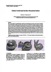
6. Repeat Steps 4 and 5 until in Step 5, the updated target curvature is close to the current one within a threshold for every boundary vertex. Uniform flat metrics are demonstrated in Figs. 4, 5, 6, and 8. In Fig. 9, we demonstrate our algorithm using a genus 3 sculpture model. The surface has one boundary, where the different positions of the boundary are marked in green in the top and bottom rows. We set the total boundary curvature to 2πχ(Σ) = −10π and calculate its uniform flat metric. Then we select a set of homology basis shown in the first three columns as blue curves. The surface is sliced along the
7
Figure 5. Surface signatures induced by the uniform flat metrics. The center of circles and the radii are surface signatures, which are conformal invariants. can be mapped onto the surface as shown in the rightmost frame. In the texture mapping, the parts of the texture corresponding to the interiors of the circles are not mapped onto the surface.
vature of singularities. 1-form can only map the boundaries to straight lines. Ricci flow can design the boundary curvatures. Ricci flow is a generalization of circle packing. Conventional circle packing only handles tangent circles and uses the gradient descend method, whereas Ricci flow handles intersecting circles and can adopt Newton’s method. Therefore, Ricci flow is more general and efficient. Circle pattern is a variation of circle packing. Both Ricci flow and circle pattern support Newton’s method for optimizing convex energies. They are Legenre dual to each other [20]. Circle pattern computes angle structures, while Ricci flow computes metrics. The framework of Ricci flow can be applied for both discrete and continuous surfaces. Circle pattern can only be applied in the discrete setting.
6. Performance We tested our algorithm on the Windows platform with 3.6 GHz CPU and 3.00 GB of RAM. In the implementation, we did not use any software package for optimization and built the software tools from scratch. As provided with the theory of Ricci flow, for all models in our experiments, the computational process is convergent and stable, where the maximum curvature error decreases exponentially. The computation time heavily depends on the geometries and the boundary conditions. If the area distortion is high, the process is more time consuming. We believe that the relation between the time cost and the area distortion is non-linear. For example, computing the uniform flat metric of the David head (30k faces) with zero boundary curvature in Fig. 4 takes 90 seconds and the embedding takes 2.5 seconds. On the other hand, computing the flat metric for the rocker arm model with 30K faces in Fig. 2 takes 300 seconds and the embedding takes 2.5 seconds. The setting of Ricci flow makes it feasible to improve the computational efficiency using a hierarchical method. In the future, we will test this approach.
Future directions Although for the purpose of parameterization, the target curvature is zero on almost every vertex, Ricci flow can calculate the conformal metrics for arbitrary admissible target curvatures. This leads to the new applications of metric design using curvatures. We will explore this direction in the future. We will also study the problem of assigning target curvatures to minimize area distortions. Besides prescribed curvatures, other geometric constraints can be added for the parameterization. In addition, we will improve our algorithm to handle large meshes using a hierarchical method.
7. Discussion and Future Work
Appendix
Comparisons with other methods Both 1-form method and Ricci flow can handle surfaces with arbitrary topologies. A 1-form method is a linear method, while Ricci flow is a nonlinear method. The singularities on 1-forms cannot be controlled, whereas Ricci flow can control the position and cur-
Admissible curvature for a mesh Suppose Σ is a triangular mesh with a discrete metric (Γ, Φ). A vertex curvature K is admissible if there exists another metric with a different Γ but the same Φ (conformal to the original metric) which induces K. The necessary and sufficient conditions for K
8
Figure 6. Different kinds of prescribed boundary curvatures induce different kinds of uniform flat metrics and conformal mesh signatures. to be admissible are the following linear inequalities; X X Ki > − (π − φ(e)) + 2πχ(FI ), (10) vi ∈I
[10] X. Gu, S. J. Gortler, and H. Hoppe. Geometry images. ACM Transactions on Graphics (Proc. SIGGRAPH), 21(3):355– 361, 2002. [11] X. Gu and S.-T. Yau. Global conformal surface parameterization. Symposium on Geometry Processing, pages 127–137, 2003. [12] R. S. Hamilton. The Ricci Flow on Surfaces, volume 71 of Mathematics and General Relativity. American Mathematical Society, Santa Cruz, CA, 1986, 1988. [13] H. Hoppe and E. Praun. Shape compression using spherical geometry images. In N. A. Dodgson, M. S. Floater, and M. A. Sabin, editors, Advances in Multiresolution for Geometric Modelling, pages 27–46. Springer-Verlag, 2005. [14] W. H.Press, S. Teukolsky, W. T. Vetterling, and B. P. Flannery. Numerical Recipes in C++. Cambridge University Press, 2002. [15] M. Jin, F. Luo, and X. Gu. Computing surface hyperbolic structure and real projective structure. In ACM Solid and Physical Modeling Symposium, 2006. [16] M. Jin, Y. Wang, S.-T. Yau, and X. Gu. Optimal global conformal surface parameterization. In Proceedings of IEEE Visualization, pages 267–274. IEEE Computer Society, 2004. [17] L. Kharevych, B. Springborn, and P. Schr¨oder. Discrete conformal mappings via circle patterns. ACM Transactions on Graphics (Proc. SIGGRAPH), 25(2), 2006. [18] G. Leibon. Characeterizing the delaunay deompositions of compact hyperbolic surfaces. Geometry and Topology, 6:361–391, 2002. [19] B. Levy, S. Petitjean, N. Ray, and J. Maillot. Least squares conformal maps for automatic texture atlas generation. SIGGRAPH 2002, pages 362–371, 2002. [20] F. Luo. Some applications of the cosine law. Discrete Differential Geometry, march 2006. [21] U. Pinkall and K. Polhier. Computing discrete minimal surfaces and their conjugates. Experimental Mathematics, 2(1):15–36, 1993. [22] N. Ray, W. C. Li, B. Levy, A. Sheffer, and P. Alliez. Periodic global parameterization. submitted for publication, 2005. [23] I. Rivin. Euclidean structures on simplicial surfaces and hyperbolic volume. Annals of Mathematics, 139(3):553–580, 1994. [24] B. Rodin and D. Sullivan. The convergence of circle packings to the riemann mapping. Journal of Differential Geometry, 26(2):349–360, 1987.
(e,v)∈Lk(I)
where given any subset I ⊂ V , FI is the set of all faces in Σ whose vertices are in I. The link of I, denoted by Lk(I), is the set of pairs (e, v) of an edge e and a vertex v such that the end points of e are not in I, the vertex v is in I, and e and v form a triangle.
References [1] A. I. Bobenko and B. A. Springborn. Variational principles for circle patterns and koebe’s theorem. Transactions on the American Mathematical Society, 356:659–689, 2004. [2] C. Carner, M. Jin, X. Gu, and H. Qin. Topology-driven surface mappings with robust feature alignment. In IEEE Visualization, page 69, 2005. [3] B. Chow and F. Luo. Combinatorial ricci flow on surfaces. Journal of Differential Geometry, 63(1):97–129, 2003. [4] C. R. Collins and K. Stephenson. A circle packing algorithm. Comput. Geom., 25(3):233–256, 2003. [5] M. Desbrun, M. Meyer, and P. Alliez. Intrinsic parameterizations of surface meshes. Computer Graphics Forum (Proc. Eurographics 2002), 21(3):209–218, 2002. [6] M. S. Floater. Parametrization and smooth approximation of surface triangulations. Computer Aided Geometric Design, 14(3):231–250, 1997. [7] M. S. Floater and K. Hormann. Surface parameterization: a tutorial and survey. In N. A. Dodgson, M. S. Floater, M. A. Sabin, N. A. Dodgson, M. S. Floater, and M. A. Sabin, editors, Advances in Multiresolution for Geometric Modelling, Mathematics and Visualization, pages 157–186. Springer, 2005. [8] S. J. Gortler, C. Gotsman, and D. Thurston. Discrete oneforms on meshes and applications to 3D mesh parameterization. Computer Aided Geometric Design, page to appear, 2005. [9] C. Gotsman, X. Gu, and A. Sheffer. Fundamentals of spherical parameterization for 3D meshes. ACM Transactions on Graphics, 22(3):358–363, 2003.
9
[25] A. Sheffer and E. de Sturler. Parameterization of faced surfaces for meshing using angle based flattening. Engineering with Computers, 17(3):326–337, 2001. [26] A. Sheffer, B. L´evy, M. Mogilnitsky, and A. Bogomyakov. ABF++: Fast and robust angle based flattening. ACM Transactions on Graphics, 24(2):311–330, 2005. [27] W. Thurston. Geometry and Topology of 3-Manifolds. Princeton lecture notes, 1976. [28] C. D. Verdi´ere. Un principe variationnel pur les empilements de cercles. Inventiones Mathematicae, 104:655–669, 1991.
10
Figure 7. Flat metric with two interior singularities.
Figure 8. A genus one surface with three boundaries is parameterized using uniform flat metric. The three circles in each period in the second left frame correspond to the three boundaries. The texture in the second right frame is mapped onto the surface in the rightmost frame.
Figure 9. Uniform flat metric for a genus 3 sculpture model. Different boundary positions induce different metrics with different area distortions. The boundary of the surface in the top row is on the back of the child. The boundary in the bottom row is at the bottom of the sculpture. After computing the metric, the seams are computed (blue curves). The surface is sliced open along the seams and embedded onto the plane as shown in the fourth column. The last column show zoom-ins of the regions in the fourth column.
11