Connecting SystemC-AMS Models with OSCI TLM 2.0 Models Using Temporal Decoupling Markus Damm, Christoph Grimm, Jan Haase Institute of Computer Technology Vienna University of Technology, Austria
Andreas Herrholz OFFIS Institute Oldenburg, Germany
{damm|grimm|haase}@ict.tuwien.ac.at
[email protected]
Wolfgang Nebel Carl von Ossietzky University Oldenburg, Germany
[email protected]
Abstract Recent additions to the system modelling language SystemC, namely SystemC-AMS and OSCI TLM 2.0, provide more efficient ways to model systems within their respective domains. However, most of today’s embedded systems are usually heterogeneous, requiring some way to connect and simulate models from different domains. In this paper we present a first approach on how to connect SystemC-AMS models and TLM 2.0 loosely timed models using temporal decoupling. We show how certain properties of the involved Models of Computation (MoC) can be exploited to maintain high simulation performance. Using an example to show the feasibility of our approach, we could also observe a certain tradeoff between simulation performance and accuracy. Further on, we discuss semantical issues and decisions that have to be made, when models are connected. As these decision are typically application-driven, we propose a converter structure that keeps converters simple but also provides ways to model application-specifc behaviour. 1
1
Introduction
Today, a lot of research and development activities in electronic design automation focus on reducing the design productivity gap due to Moore’s Law. Traditional approaches and design languages are not efficient enough anymore to cope with the rising complexity in system design. As one result, the system modelling language SystemC is nowadays widely used for embedded hardware/software design in industry and academia. SystemC is based on C++ and available under an open source license, so it is easily extensible by other methodology specific libraries. 1 The work presented in this paper has been carried out in the ANDRES project, co-funded by the European Commision within the Sixth Framework Programme (IST-5-033511).
One of these modelling methodologies introduced with SystemC is Transaction Level Modelling (TLM) [2, 4]. TLM models the communication of processes by method calls enabling early integration of hardware and software and significantly improving simulation speed compared to cycle-accurate models. Recently, the Open SystemC Initiative (OSCI) released the second draft of its TLM 2.0 standard for public review [6]. TLM 2.0 extends the previous OSCI TLM standard by a more detailed approach for modelling bus-oriented systemson-chips, enabling easy reuse of existing models in different architectures. TLM 2.0 introduces three different modelling styles (also called coding styles) regarding the modelling of time, providing different trade-offs between simulation accuracy and speed. In the untimed modelling style, time is not modelled at all. In the loosely timed modelling style, processes are allowed to run ahead of the global SystemC simulation time (temporal decoupling). Since this modelling style is the focus of our interest, we will describe it in more detail later. Finally, when using the approximately timed modelling style, all processes run in lock-step with the global SystemC simulation time. Another SystemC extension is SystemC-AMS [7], enabling the modelling of analogue/mixed signal applications using different Models of Computation, e.g. Timed Synchronous Dataflow (TDF) for data-flow oriented models, linear electrical networks (LEN) or differential algebraic equations (DAE). SystemC-AMS focuses on executable specification rather than exact modelling providing higher simulation performance than circuit simulators while being slightly less accurate. Both of the given SystemC extensions work well in their respective domains. However, today’s embedded systems are usually heterogeneous in nature, combining components from different domains, such as digital hardware, software and analogue hardware. Therefore an efficient design flow for heterogeneous systems would require ways to combine both approaches in one joint model enabling early simulation and exploration.
Though SystemC-AMS provides means to connect AMS models with discrete-event SystemC models, these are not enough to efficiently integrate AMS models in TLMbased systems, since they stay on the signal level. In this paper, we present and discuss a first approach for a MoC converter that can be used to connect loosely timed TLM models with TDF models. To our best knowledge, there is no other published work on this topic so far. The rest of this paper is organized as follows: We start with a brief introduction of the TLM 2.0 loosely timed modelling style and the SystemC-AMS TDF computational model. This is followed by a discussion on how these two models can be connected by exploiting certain similarities to maintain their simulation efficiency. We then present the general structure of converters from TLM to TDF and vice versa in Sections 5 and 6, and present an example where they are used in Section 7. Section 8 discusses semantical issues that may arise when TDF and TLM models are coupled and how these issues can be handled using a structured modelling approach. We conclude in Section 9.
2
OSCI TLM 2.0 loosely timed modelling style
The draft 2 of the OSCI TLM 2.0 standard [6] introduces the so called loosely timed modelling style (LTTLM). In this modelling style, a non-blocking method interface is used, where initiator processes generate transactions (the payload) and send them using a method call to target processes. The speciality of this modelling style is the possibility to annotate a transaction with a time delay d to mark it (in the case of d > 0) as a future transaction. That is, the loosely timed modelling style allows initiator processes to warp ahead of simulation time. The target processes, on the other hand, must deal with these future transactions accordingly. They have to store them in a way such they can access and process delayed transactions at the right time. For example, the payload event queue (PEQ) [1], foreseen by the TLM 2.0 standard, can be used for this. The idea of this approach is that context switches on the simulation host system (generally triggered by wait() statements) are reduced and thus simulation performance is gained. Instead of letting initiator and target repeatedly produce and process a transaction respectively, an initiator can produce a chunk of transactions in advance, which is then processed by a target (ideally) at once. However, this may lead to time-twisted transactions, i.e. the order of arrival of two transactions at one target is different from their temporal order. If the processing of these transactions is not synchronized, this may lead to causal errors. The loosely timed modelling style basically allows processes to run according to their own, local simulation time. To organize this, TLM 2.0 provides the facility of the quantum keeper. Processes can use the quantum keeper to keep track of their local timewarp, and yield to the SystemC simulation kernel after a certain time quan-
tum is used. Typically, a smaller time quantum will reduce the chance of causal errors while a greater quantum increases the simulation performance. So using the quantum keeper, the tradeoff between simulation performance and accuracy can be controlled.
3
SystemC-AMS TDF
The main Model of Computation (MoC) provided by SystemC-AMS is the Timed Synchronous Dataflow (TDF) MoC. It is a timed version of the (originally untimed) Synchronous Dataflow (SDF) MoC [5], where processes communicate via bounded fifos. The number of data tokens produced and/or consumed by a process (the data rate) is constant for all process firings. For example, consider a process which has two inputs with data rates 2 and 3, and an output with data rate 4. Every time this process is fired, it will consume 2 and 3 tokens from its two inputs and will produce 4 tokens at its output. The advantage of SDF is that the schedule of process execution can be computed in advance, such that the simulation kernel is only engaged with executing this static schedule, which makes the simulation of SDF models very fast. The speciality of the SystemC-AMS TDF MoC is that a certain time span (the sampling period) is associated with token consumption and production. The sampling period is an attribute of the (input or output) TDF port classes, which are analogous to the SystemC sc_in and sc_out classes, respectively. Via TDF ports, TDF modules are connected to each other by TDF signals. Again, these facilities are correspondent to the sc_module and sc_signal classes. A TDF module encapsulates the actual process as a standard method called sig_proc(). In the current SystemCAMS prototype, the sampling period has to be set only at one TDF port of one TDF module of a connected set of TDF modules (also called TDF cluster). The sampling periods of all other TDF ports within the cluster are then a result of this one given sampling period. For example, if the sampling period of an input port p1 of a TDF Module M1 is set to 2 ms, with a data rate of 3, the consumption of one token takes 2 ms. such that the consumption of all 3 tokens takes 6 ms. If M1 contains also an output port p2 with data rate 2, the sampling period of p2 is 6ms divided by the datarate of 2, resulting in 3 ms. An input port p3 of a TDF module M2 which is connected to p2 via a TDF signal now also has a sampling period of 3 ms, regardless of its data rate.
4
Connecting LT-TLM and TDF
At a first glance, bringing these two approaches together seems to be futile. On the one hand, there is the loosely timed TLM approach with its local time warps decoupled from the global simulation time. On the other hand, we have the strictly timed TDF approach which runs at an unstoppable pace. But by taking a closer look at how the TDF simulation works when using a static
schedule (as it is the case with the current SystemC-AMS prototype), we find surprising similarities. The SystemC-AMS simulation kernel is using its own simulation time, whose current value is returned by the TDF module method sca_get_time() (from now on denoted by tT DF ). The current SystemC simulation time (from now on denoted by tDE ) is returned by the DE module method sc_time_stamp(). By DE, we denote the discrete event MoC implemented by the SystemC simulation kernel, while a DE module denotes the sc_module-instances. If a pure SystemC-AMS TDF model is used in a simulation, the SystemC-AMS simulation kernel is blocking the DE kernel all the time, so the DE simulation time doesn’t proceed at all. However, there might be a need to connect and synchronize TDF modules to DE modules. SystemC-AMS provides converter ports for this cause, namely sca_scsdf_in and sca_scsdf_out. They can be used within TDF modules to connect to instances of the SystemC discrete event sc_signal. If there is an access to such a port within the sig_proc() method of a TDF module, the SystemCAMS simulation kernel interrupts the execution of the static schedule of TDF modules and yields to the SystemC DE simulation kernel, such that the DE part of the model can now execute, effectively proceeding tDE until it is equal to tT DF . Now, the DE modules reading from signals driven by TDF modules can read their new values at the right time, and TDF modules reading from signals driven by DE modules can read their correct current values. Figure 1 shows an example using the TDF module M1 from Section 3. The data tokens consumed are on the left axis, and those produced are on the right axis. The numbers beneath the tokens denote the time (in ms) at which the respective token is valid. The time spans above the tokens indicate the values of tT DF when the respective token are consumed resp. produced. The time spans below indicate the according values for tDE . At the beginning of the example, tT DF > tDE already holds, until tT DF = 38ms. Then the SystemC-AMS simulation kernel initiates synchronization, for example because M1 contains a converter port which it accesses at that time, or because another TDF module within the same TDF cluster accesses its converter port. tTDF
38 ms
26 ms
32 ms
Converting from LT-TLM to TDF
The principal idea of a TLM→TDF converter is to take write-transactions (i.e. with a command set to TLM_WRITE_COMMAND) and stream their data to a TDF signal. However, we are confronted with several difficulties. First of all, we can’t expect the data from the TLM side to arrive at certain rates, even if we take the time warp into account. We might get huge amounts of data within short time spans, and almost no data for long time spans. Nevertheless, we have to feed an unstoppable data token consumer, namely the TDF reading side. The obvious solution for this problem is to use an internal fifo within the converter to buffer the incoming data. If a transaction causes a buffer overflow (when the internal buffer is chosen to be of a fixed size), it is returned with an error response. Currently, we set the response status to TLM_GENERIC_ERROR_RESPONSE, but we might consider using a generic payload extension to make this more specific. If, on the other hand, the buffer is empty, default value(s) are written to the TDF side to fill the gap(s) (e.g. 0). DE-module
30
32
20 ms
34
36
38
40 38 ms
42
ms
p1 2 ms rate 3
p2 3 ms rate 2
synchronization tTDF ↔ tDE
sig_proc() port to port
38 ms
TDF-module M1 28
TDF-module
nb_transport()
tlm_nb_target_socket 26
29
32
20 ms
35
38
41 ms
38 ms
Figure 1. Example for the relation of tDE to tT DF with synchronization The important conclusion is that TDF modules also use a certain time warp. In general, TDF modules run ahead of SystemC simulation time, since tT DF ≥ tDE always holds. Further time warp effects result from using
TDF out DE-module DE out
DE-signal
TDF out
TDF-signal
tDE
32 ms
5
method call
token valid at 26
26 ms
multi-rate data flow. When a TDF module has an input port with data rate > 1 it also receives "future values" with respect to tDE , and even tT DF . When a TDF module has an output port with data rate > 1, it also sends values "to the future" with respect to tDE and tT DF . The difference to TLM is that the effective local timewarps are a consequence of the static schedule, with the respective local time offsets only varying because of interrupts of the static schedule execution due to synchronization needs. In the following two Sections we describe how the streaming data of TDF signals can be converted to TLM 2.0 transactions and vice versa, effectively proposing general TLM2↔TDF converters. We do this in a way such that the temporal decoupling approach of the TLM 2.0 loosely timed modelling style is exploited to maintain a high simulation performance. The transaction class used will always be the TLM 2.0 generic payload.
TDF-DE in converter
Figure 2. The TLM→TDF converter architecture Another advantage of using an internal buffer is that the size of the data section of the write-transactions can
be set independent from the data rate of the TDF output of the converter. Especially, the transaction data size can vary over the course of the simulation. Another problem, however, arises due to the delays of the transactions. It can’t be guaranteed that after the arrival of a transaction T1 , which is ready at e.g. tDE = 50ms, that there won’t be a transaction T2 which arrives later, but is ready at e.g. tDE = 40ms. That is, transactions can arrive with twisted time warps, since they might have emerged from different initiators, or from one initiator producing such twisted time warped transactions (there is no rule within TLM 2.0 which prohibits this). Therefore, we can’t write the transaction data to the buffer right away. Instead, we write the transaction to a PEQ, where the transactions are stored in the order of their procession time, such that these delay twists are resolved. When the local time of the converter has proceeded far enough for a transaction in the PEQ to be processed, its data gets written to the buffer. For this, the PEQ is checked for transactions with a time stamp smaller or equal to the current local time of the converter at every sig_proc() execution. Another issue we have to deal with is synchronization. Since the converter is a TDF module, it might run way ahead of tDE , and the initiators feeding the converter might not have had the chance to produce transactions sufficiently, even if they would be ready by the time of the converter’s sig_proc() execution. Therefore, if there are no transactions available in the PEQ when the sig_proc() is processed, and the buffer also holds not enough data for the output, the SystemC simulation kernel must get the chance to catch on. This is done by connecting the converter to a sc_signal using a SystemC-AMS converter port. If a reading access is now performed on this converter port, the SystemC-AMS simulation kernel interrupts the procession of the static schedule, and the SystemC simulation kernel regains control and can proceed the SystemC simulation (including the TLM initiator modules) until tDE = tT DF . Figure 2 shows an overview of the architecture of the proposed converter. The core is a TDF-module, which contains the PEQ, the buffer, and the port to the TDF side. It is encapsulated within a DE-module, which implements the TLM 2.0 nonblocking transport interface. For synchronization, the TDF module is connected to a DE-signal via a SystemC-AMS converter port. Note that the DE-signal needs no driver; simply accessing it from within the TDF module is sufficient to trigger synchronization.
When converting from TDF to TLM, we want to bundle the streaming TDF data into the data section of a transaction and send it to the TLM side. This would be an easy and straightforward task if we would consider the converter (i.e. the TDF side) to act as an TLM initiator. In this case, the transaction’s command would be set to TLM_WRITE_COMMAND, and the delay of the trans-
nb_transport()
sig_proc() port to port TDF in
tlm_nb_target_socket TDF in DE-module TDF-DE in converter
DE-signal
method call
Converting from TDF to LT-TLM
DE-module TDF-module
TDF-signal
6
action could be set to the difference of tDE and the valid time stamp of the last token sent via the transaction (i.e. tT DF + token number·sampling period). However, despite its striking simplicity, the TDF models we focus on here just provide streaming input to the TLM side, and the idea of such models acting as a TLM initiator is as realistic as an A/D converter acting as a bus master. Also, the address the transaction is sent to would basically be static throughout the simulation, since we don’t get addresses from the TDF side (at least not in an obvious manner). As a consequence, the converter would need to read address manipulating transactions coming from the TLM side, too, in order to be useful. There are useful applications for TDF models acting as TLM initiators, and we get back to this topic in Section 8. Nevertheless, for now we chose a conversion approach where the initiators are again on the TLM side. That is, TLM initiators send read-transactions (i.e. with the command set to TLM_READ_COMMAND) to the converter, which copies the data tokens it receives from the TDF side into the data section of the transaction and returns it. The advantage of this approach is that it is pretty similar to the TLM→TDF conversion direction. For example, the converter needs an internal buffer to store the incoming TDF data tokens, for similar reasons as discussed in Section 5. Here, the TLM side might request data of varying length at varying times, while the TDF side provides data at an unstoppable pace. Therefore, an internal fifo is used again. We also use a PEQ to store the incoming transactions, such that time delay twists are resolved. In this case, the standard TLM 2.0 PEQ is used, which produces an event when a transaction within the queue is ready. In that case, the transaction is taken from the queue, and it is checked whether the internal buffer provides sufficiently many data tokens to fill the transaction’s data section. Here, we also have to make sure that we don’t return "future" tokens from the transaction’s point of view. Note that the presence of such tokens in the internal buffer is perfectly possible when using multirate data flow. If enough valid data tokens are present, the transaction is returned with them. If not, it is returned with an error response status.
DE out
Figure 3. The TDF→TLM converter When the internal fifo is chosen to be of finite
size, buffer overflows can occur. Therefore, at every sig_proc() execution, it is checked whether the internal buffer contains enough space to take the next chunk of data tokens provided by the TDF side. If not, the converter yields to the SystemC simulation kernel with the same converter port access technique described in Section 5. This gives the TLM side the chance to produce more reading transactions, and might proceed tDE far enough for transactions in the PEQ to become ready. If there is still not enough space in the internal buffer, the surplus data tokens are simply discarded and a warning is raised. As it can be seen in Figure 3, the architecture of the TDF→TLM converter is pretty similar to the architecture of the TLM→TDF converter. Since the TDF part now does not need to access the PEQ, it is contained in the toplevel DE-module.
7
Example system
Regarding the simulation speed, we measure the number of context switches in the TLM initiators, since a high number of context switches usually increases simulation time. That is, every point in simulation time the simulator switches to the process of one specific DSP counts as one context switch. We simulated about 16 minutes of time, in which about 12,000 data packages with 128 values were received by the drains. The sampling period of the sources was 1 ms. Figure 5 shows the results. The curve starting to the left with a value of about 600,000 is the number of context switches, while the other curve shows the number of errors (i.e. data package twists) with a maximum of about 1,200. As it can be seen, even a small timewarp reduces the number of context switches drastically, while larger timewarps don’t reduce the context switches much more, but lead to errors. In fact, using a timewarp up to 100 ms resulted in no errors at all, but led to 20 times less context switches. 700000
To test our conversion approach, we implemented an example system containing two TDF sources, two TDF drains, three TLM digital signal processing (DSP) modules and a TLM bus (see Figure 4). The idea of this system is that the data coming from sourcei is processed by any of the DSPs, and the results are then passed to the respective draini (i = 1, 2). Here, the exact nature of the computations performed by the DSPs were not the focus of our interest. However, a possible example would be a software defined radio, where the TDF sources would provide data to be modulated (or demodulated). The modulation (or demodulation) schemes to be applied to the source data could be different for every source, but every DSP provides the capabilities to perform them. That is, every DSP checks the sources for new data, reads them, processes them accordingly, and writes the results to the appropriate drain. 1
2
3
1
2
1
2
Figure 4. Example system Our interest in this model is to demonstrate the functional correctness of our converters and to observe accuracy / simulation speed tradeoffs, typical for loosely timed TLM models. The loss of accuracy in this case manifests itself in data packages arriving at the signal drains in the wrong order. This is possible in principle, since the DSPs run independently from each other. Nevertheless, when the DSPs run in approximately timed mode (i.e. their time warp is set to 0 and they run in lock-step with SystemC simulation time), the procession delay will make sure that the data package order is preserved. However, when we allow the DSPs to warp ahead in time locally, such data package twists can occur.
# context switches
# errors
1400
600000
1200
500000
1000
400000
800
300000
600
200000
400
100000
200
0
0
100
200
300
400
500
0 600 timewarp (ms)
Figure 5. Speed vs. accuracy tradeoff in example system
8
Discussion of semantical issues
The focus of Section 5 and Section 6 was to provide a sound technical basis for interoperability of SystemCAMS models with TLM 2.0 models using temporal decoupling. However, there are certain semantical issues requiring discussion. One issue concerns the buffers within the converters. Should they be of limited size or virtually be unlimited? Also, is there a canonical way, how the converters should behave when their buffers run full or empty? A similar question arose in previous work [3] on automatic conversion between Kahn Process Network (KPN) models and TDF models. The approach chosen there was to allow the designer to specify the buffer size. In the finite buffer case, several options can be set for raising an error, return a default value or the last value which could be read from the buffer (empty buffer case), or to discard either the new value or the oldest value in the buffer (full buffer case). The same could be used here, as the decision how to dimension the buffer is basically application specific. For example, there might be cases where a converter’s buffer directly relates to a buffer that will also be present in the final implementation, so it would make sense to have the size of the converter buffer limited. Also a
designer would like to make sure that there are always enough tokens available as inputs to the TDF model and he wants the converter to throw an exception or give at least a warning if there are no more tokens available. Another open question was briefly mentioned in Section 6, namely whether a TDF model can be a TLM initiator or not. In general, there is no reason why a TDF model should not act like an initiator or master. Imagine a TDF model simulating an signal processing algorithm that is later to be implemented on a DSP. The algorithm might regularly read data from a memory and write its result back to the memory, so later the DSP will become a bus master, periodically generating read and write transactions. However in many cases the TDF model will usually be a target or slave, like e.g. a D/A converter only reacting to requests from other initiators. As it can be seen, all resolutions of the issues come down to application specific properties and decisions. So the designer always has to specify the behaviour he expects from the converters. Integrating all of these possible behaviours within one configurable converter would potentially result in a quite complex and difficult to modelling element. Therefore we propose a different approach: For keeping the converter simple and elegant while still having the full degree of application-defined behaviour, it is best to split the converter in two parts: One application independent part (the basic converter), implementing a reduced and well-defined subset of the converter semantics. And one application specific part (the wrapper), implementing the application specific behaviour on top of these semantics. While the basic converter provides the coupling of the two involved Models of Computation, the wrapper can also be designed, such that it implements the interface of an AMS component as it will be found in the final architecture. So for example, if the TDF model should act like a bus master, the wrapper could also be implemented as a TLM initiator. The basic converter could then be provided as a ready-to-use element while for the wrapper the designer would be required to specify the expected behaviour. We think that to finally define the basic converter’s semantics would require an indepth analysis of typical application use cases. Also, formalizing the semantics of the conversion could help to prove that all application specific behaviour can be mapped in general to the restricted set of the basic converter. However, this is out of the scope of this paper and will be done in future work.
9
Conclusion and future work
In this paper, a first approach on how to connect SystemC-AMS models with loosely timed TLM 2.0 models using temporal decoupling was presented, with the focus on the SystemC-AMS side acting as a streaming data producer and/or consumer. It was shown that the loosely timed modelling style of TLM 2.0 can be exploited efficiently to fit with SystemC-AMS’s TDF, preserving the high simulation performance of both Mod-
els of Computation. We described generic converter elements implementing our approach. A small example model was implemented which indicated the converters functional correctness, while the general simulation performance / accuracy tradeoff typically found in loosely timed TLM models could still be observed. We concluded with discussing semantical issues that arise when defining the conversions behaviour. As these issues are typically application specific, we proposed a structured approach separating the conversion in a general and an application dependent part. The purpose of this paper was to present a first technical feasibility analysis of TLM↔TDF conversion. We were able to show, that the idea of having TLM initiators running in advance of simulation time shows some similarities to how TDF is simulated by the SystemCAMS kernel and helps to solve the synchronization task. In principle, approximately timed TLM models could be connected to TDF models using the same converter approach. However this would not show the same simulation benefit as AT models are not allowed to run in advance. Future work in this area will focus on two aspects: To formalize the conversion problem at hand more rigidly, possibly including a more formal description of the TLM 2.0 loosely timed modelling style. And to explore and implement a more structured and sophisticated TLM↔TDF conversion approach as outlined in Section 8 by analysing typical application use cases for the interfacing of purely digital systems with analog/mixed signal components.
References [1] J. Aynsley. OSCI TLM2 User Manual. Technical report, Open SystemC Initiative, 2007. [2] L. Cai and D. Gajski. Transaction level modeling in system level design. In Technical Report 03-10. Center for Embedded Computer Systems, University of California, Irvine, 2003. [3] M. Damm, F. Herrera, J. Haase, E. Villar, and C. Grimm. Using Converter Channels within a Top-Down Design Flow in SystemC. In Proceedings of the Austrochip 2007, 2007. [4] F. Ghenassia. Transaction-Level Modeling with SystemC: TLM Concepts and Applications for Embedded Systems. Springer-Verlag New York, Inc., Secaucus, NJ, USA, 2006. [5] E. A. Lee and D. G. Messerschmitt. Static scheduling of synchronous data flow programs for digital signal processing. IEEE Transactions on Computers, C-36(1):24 – 35, 1987. [6] Open SystemC Initiative. OSCI TLM2.0 draft2. http: //www.systemc.org. [7] A. Vachoux, C. Grimm, and K. Einwich. Towards Analog and Mixed-Signal SoC Design with SystemC-AMS. In IEEE International Workshop on Electronic Design, Test and Applications (DELTA’04), Perth, Australia, 2004.