AbstractâWe study connectivity and transmission latency in wireless networks with unreliable links from a percolation-based perspective. We first examine static ...
This full text paper was peer reviewed at the direction of IEEE Communications Society subject matter experts for publication in the IEEE INFOCOM 2008 proceedings.
Connectivity and Latency in Large-Scale Wireless Networks with Unreliable Links Zhenning Kong and Edmund M. Yeh Department of Electrical Engineering Yale University New Haven, CT 06520, USA Email: {zhenning.kong, edmund.yeh}@yale.edu Abstract—We study connectivity and transmission latency in wireless networks with unreliable links from a percolation-based perspective. We first examine static models, where each link of the network is functional (active) with some probability, independently of all other links, where the probability may depend on the distance between the two nodes. We obtain analytical upper and lower bounds on the critical density for phase transition in this model. We then examine dynamic models, where each link is active or inactive according to a Markov onoff process. We show that a phase transition also exists in such dynamic networks, and the critical density for this model is the same as the one for static networks under some mild conditions. Furthermore, due to the dynamic behavior of links, a delay is incurred for any transmission even when propagation delay is ignored. We study the behavior of this transmission delay and show that the delay scales linearly with the Euclidean distance between the sender and the receiver when the network is in the subcritical phase, and the delay scales sub-linearly with the distance if the network is in the supercritical phase.
I. I NTRODUCTION Large-scale wireless networks for the gathering, processing, and dissemination of information have become an important part of the modern communication infrastructure. Traditionally, the performance of wireless networks has been examined under the assumption of maintaining full connectivity (or kconnectivity) [1], [2]. Here, the system ensures that any pair of nodes in the network are connected by a path (or k paths). In large-scale wireless networks exposed to severe natural hazards, enemy attacks, and resource depletion, however, this full connectivity criterion may be overly restrictive or impossible to achieve. In this paper, we view the connectivity of large-scale wireless networks from a different perspective. One simple measure of the network functionality is the fraction of nodes in the largest connected component of the network: nodes in that component can communicate with an extensive portion of the network, while those in smaller components can communicate only with at most a few other nodes. For instance, if a wireless sensor network is able to collect information from almost the entire coverage area even after a substantial number of sensor failures, then the network is considered to be functional. On the other hand, if after many sensor failures, the sensor 1 This research is supported in part by National Science Foundation (NSF) Cyber Trust grant CNS-0716335, and by Army Research Office (ARO) grant W911NF-07-1-0524.
network breaks down into isolated parts where even the largest component can reach only a few sensors, then the network is not considered to be functional. From this perspective, the characterization of network connectivity corresponds to the study of the qualitative and quantitative properties of the largest component. A powerful technique for this study comes from the mathematical theory of percolation [3]–[6]. Recently, percolation theory, especially continuum percolation theory, has become a useful tool for the analysis of coverage, connectivity, capacity and latency in large-scale wireless networks [1], [7]–[14]. To intuitively understand percolation processes in largescale wireless networks, consider the following example. Suppose a set of nodes are uniformly and independently distributed at random over an area. All nodes have the same transmission radius, and two nodes within a transmission radius of each other are assumed to communicate directly. At first, the nodes are distributed according to a very small density. This results in isolation and no communication among nodes. As the density increases, some clusters in which nodes can communicate with one another directly or indirectly (via multi-hop relay) emerge, though the sizes of these clusters are still small compared to the whole network. As the density continues to increase, at some critical point a huge cluster containing a large portion of all nodes in the network forms. This phenomenon of a sudden and drastic change in the global structure is called a phase transition. The density at which phase transition takes place is called the critical density [3]– [6]. A fundamental result of continuum percolation concerns such a phase transition effect whereby the macroscopic behavior of the system is very different for densities below and above the critical density λc . For λ < λc (subcritical), the connected component containing the origin (or any other node) contains a finite number of points almost surely. For λ > λc (supercritical), the connected component containing the origin (or any other node) contains an infinite number of points with a positive probability [3]–[6]. Due to noise, fading and multi-user interference, communication links in wireless networks are unreliable. Even when two nodes lie within each other’s transmission range, a viable communication link may not exist between the two nodes due to path-loss and fading. To capture this effect, we first study percolation processes in wireless networks with static
978-1-4244-2026-1/08/$25.00 © 2008 IEEE
This full text paper was peer reviewed at the direction of IEEE Communications Society subject matter experts for publication in the IEEE INFOCOM 2008 proceedings.
unreliable links, where each link of the network is functional (i.e., active) with some probability (which may depend on the distance between the two nodes) independently of all other network links. This is a specific case of the so-called random connection model [5]. We employ the cluster coefficient method introduced recently in [15], [16], and coupling methods to obtain lower and upper bounds on the critical density for this model. In wireless environments with time-varying channels, each link may dynamically switch between the active and inactive states. To investigate the effect of this dynamic behavior on percolation-based connectivity, we further study percolation processes in wireless networks with dynamic unreliable links. We show that a phase transition exists in these dynamic networks under certain conditions, and the critical density for this model is the same as the one for static networks with the same parameters. Furthermore, due to the dynamic behavior of links, a delay is incurred for any transmission even when propagation delay is ignored. We study the behavior of this transmission delay by modeling the problem as a first passage percolation [17], [18] process on random geometric graphs. We show that ignoring propagation delay, the message delay scales linearly with the Euclidean distance between the sender and the receiver when the resulting network is in the subcritical phase, and the delay scales sub-linearly with the distance if the resulting network is in the supercritical phase. This paper is organized as follows: in Section II, we outline some preliminary results for random geometric graphs and continuum percolation. In Section III, we study wireless networks with static unreliable links and obtain lower and upper bounds on the critical density. In Section IV, we introduce a model for wireless networks with dynamic unreliable links, and study percolation-based connectivity and transmission delay performance in such dynamic networks. In Section V, we present simulation results on percolation phenomenon and transmission delay. Finally, in Section VI, we conclude the paper. II. R ANDOM G EOMETRIC G RAPHS AND C ONTINUUM P ERCOLATION A. Random Geometric Graphs We use random geometric graphs to model wireless networks. Assume a communication link exists between two nodes if the distance between them is sufficiently small, so that the received power is large enough for successful decoding. Let � · � be the Euclidean norm, and f be some probability density function (p.d.f.) on Rd . Let X1 , X2 , ..., Xn be independent and identically distributed (i.i.d.) d-dimensional random variables with common density f , where Xi denotes the random location of node i in Rd . The ensemble of graphs with undirected links connecting all those pairs {xi , xj } with �xi − xj � ≤ r, r > 0, is called a random geometric graph [6], and denoted as G(Xn , r). In the following, we consider random geometric graphs G(Xn , r) in R2 , with X1 , X2 , ..., Xn distributed i.i.d. accord� ing to a uniform distribution in a square area A = [0, nλ ]2 .
Let A = |A| be the area of A. There exists a link between two nodes i and j if and only if i lies within a circle of radius r around xj . Ignoring border effect, the probability for the 2 λπr 2 existence of such a link is given by Plink = πr A = n . It follows that the degree of any given node has the distribution Binomial(n − 1, Plink ), so that the mean degree of each node 2 is (n − 1)Plink = (n−1)λπr . n n As n and A both become large with the ratio A = λ kept constant, each node has an approximately Poisson degree distribution [6], [19] with an expected degree (n − 1)λπr2 = λπr2 . (1) µ = lim n→∞ n n = λ fixed, In this case, as n → ∞ and A → ∞ with A G(Xn , r) converges in distribution to an (infinite) random geometric graph G(Hλ , r) induced by a homogeneous Poisson point process with density λ > 0. Due to the scaling property of random geometric graphs [5], [6], in the following, we focus on G(Hλ , 1). B. Critical Density for Random Geometric Graphs Let Hλ,0 = Hλ ∪ {0}, i.e., the union of the origin and the infinite homogeneous Poisson point process with density λ. Note that in a random geometric graph induced by a homogeneous Poisson point process, the choice of the origin can be arbitrary. The critical density is defined as follows [6]: Definition 1: For G(Hλ,0 , 1), the percolation probability p∞ (λ) is the probability that the component containing the origin has an infinite number of nodes of the graph. The critical density λc is defined as λc = inf{λ > 0 : p∞ (λ) > 0}. It is known that if λ > λc , then there exists a unique connected component containing Θ(n) nodes2 in G(Xn , 1) a.a.s.3 This largest connected component is called the giant component [5]. A fundamental result of continuum percolation states that 0 < λc < ∞. Exact values of λc and p∞ (λ) are not yet known. Simulation studies show that 1.43 < λc < 1.44 [20], while the best rigorous bounds are 0.7698 < λc < 3.372 [5], [15], [16], [21]. The best lower bound (0.7698) on λc was recently derived using an analytical method involving the clustering phenomenon in random geometric graphs [15], [16]. Here, if node i is close to node j, and node j is close to node k, then i is typically also close to k. The clustering phenomenon captures the dependence among links in random geometric graphs. Definition 2: Given distinct nodes i, j, k in G(Hλ , 1), the cluster coefficient C is the conditional probability that nodes i and j are adjacent4 given that i and j are both adjacent to node k. 2 We say f (n) = O(g(n)) if there exists n > 0 and constant c such that 0 0 f (n) ≤ c0 g(n) ∀n ≥ n0 . We say f (n) = Ω(g(n)) if g(n) = O(f (n)). Finally, we say f (n) = Θ(g(n)) if f (n) = O(g(n)) and f (n) = Ω(g(n)). 3 An event is said to be asymptotic almost sure (abbreviated a.a.s.) if it occurs with a probability converging to 1 as n → ∞. 4 In an undirected graph G = (V, E), V and E denote the set of nodes and links respectively. Given u, v ∈ V , we say u and v are adjacent if there exists a link between u and v.
This full text paper was peer reviewed at the direction of IEEE Communications Society subject matter experts for publication in the IEEE INFOCOM 2008 proceedings.
By geometric calculation, the cluster coefficient can be √ found as C = 1 − 34π3 [22]. III. P ERCOLATION IN W IRELESS N ETWORKS WITH S TATIC U NRELIABLE L INKS A. Wireless Networks with Static Unreliable Links Random geometric graphs are good simplified models for wireless networks. However, because of noise, fading and interference etc., wireless communication links between two nodes are usually unreliable. We use the bond percolation model on random geometric graphs to study percolationbased connectivity of large-scale wireless networks with static unreliable links. Given a random geometric graph G(Hλ , 1), let each link of G(Hλ , 1) be active (independent of all other links) with probability pe (d) which may depend on d, where d = �xi −xj � ≤ 1 is the length of the link (i, j). The resulting graph consisting of all active links and their end nodes is denoted by G(Hλ , 1, pe (·)). This model is also known as the random connection model in continuum percolation theory [5]. It is known that there exists a critical density λc (pe (·)) for this model. That is, when λ > λc (pe (·)), G(Hλ , 1, pe (·)) is percolated, i.e., there exists a giant component in G(Hλ , 1) consisting of active links and their end nodes a.a.s., and when λ < λc (pe (·)), G(Hλ , 1, pe (·)) is not percolated, i.e., there is no giant component in G(Hλ , 1) consisting of active links and their end nodes a.a.s. We say pe (·) is an effective connection probability function if pe (·) satisfies the following conditions: (i) 0 ≤ pe (x) ≤ 1 for all x ∈ (0, +∞); (ii) for all x ∈ (1, +∞), pe (x) = 0; (iii) pe (·) is continuous on (0, 1] and pe (0+ ) > 0. The first requirement reflects the fact that pe (·) is a probability, and the second requirement reflects the power constraint at each node. Although the third one is a technical requirement needed to obtain the upper bound on the critical density, it is also quite practical in real wireless networks. B. Bounds on the Critical Density In the following theorem, we provide analytical lower and upper bounds on λc (pe (·)). Theorem 1: If pe (·) is an effective link probability function, then 1 (2) ≤ λc (pe (·)), ˜ α(1 − C)π where C˜ is given by � � 1 �� 1−h � 1 2 2πxp(x)dx + 2θxp(x)dx hdh, C˜ = π 0 0 1−h � 2 2 � (3) �1 −1 , and α = 2 0 xpe (x)dx. where θ = cos−1 x +h 2xh Furthermore, almost surely, λc , (4) λc (pe (·)) ≤ β where λc is the critical density of G(Hλ , 1) and β = sup{r02 � : pe (x) ≥ �, ∀x ∈ (0, r0 ], r0 ≤ 1}.
We employ the cluster coefficient method introduced in [15], [16] to derive the lower bound on λc (pe (·)). To begin, we need to calculate the cluster coefficient C˜ of G(Hλ , 1, pe (·)). The detailed analysis and derivation are given in Appendix A. To prove the second part, we also need the following monotonic property for λc (pe (·)), which can be proved by coupling methods easily. Proposition 2: Let λc (pe (·)) and λc (p�e (·)) be the critical densities for G(Hλ , 1, pe (·)) and G(Hλ , 1, p�e (·)), respectively. Then, if p�e (x) ≤ pe (x), ∀x ∈ (0, 1], we have λc (pe (·)) ≤ λc (p�e (·)). Proof of Theorem 1: In G(Hλ , 1, pe (·)), the underlying point process is� homogeneous Poisson, and the mean degree is 1 µ = λ2π 0 xpe (x)dx = λπα. The probability of each link in G(Hλ , 1, pe (·)) being active or not is independent of all other links. By Theorem 1 and Corollary 1 in [15], in order to guarantee percolation, it is required that απλc (pe (·)) > 1−1C˜ , where C˜ is the cluster coefficient of G(Hλ , 1, pe (·)). Consequently, the lower bound follows. Now we show the upper bound. Since pe (0+ ) > 0 and pe (·) is continuous on (0, 1], there exists � > 0 and 0 < r0 ≤ 1 such that for any x ∈ (0, r0 ], pe (x) ≥ �. Let β = sup{r02 � : pe (x) ≥ �, ∀x ∈ (0, r0 ], r0 ≤ 1}. Consider a new model G(Hλ , 1, p�e (·)), where p�e (·) is a truncated version of pe (·): � pe (x) ∀x ∈ (0, r0 ] p�e (x) = 0 ∀x ∈ (r0 , +∞) By the monotonic property of λc (pe (·)) (Proposition 2), it is easy to see that whenever G(Hλ , 1, p�e (·)) is percolated, the original model G(Hλ , 1, pe (·)) must be percolated. Now consider a new model G(Hλ , r0 , �), i.e., a random geometric graph with radius r0 where each link is active with probability �. Then, G(Hλ , r0 , �) is a subgraph of G(Hλ , 1, p�e (·)). This implies that whenever G(Hλ , r0 , �) is percolated, so is G(Hλ , 1, p�e (·)). Now consider a site percolation process on G(Hλ , r0 ) where λc each node is active with probability � = λλ1 > λr 2 . In other 0 words, we let a node in G(Hλ , r0 ) be active with probability � independently of each other, and keep all the associated links active. Denote the resulting graph by G� . According to the Thinning Theorem [5], [6], G� is a random geometric graph with density λ1 > λc /r02 . Hence G� is percolated. It is known that the critical probability for site percolation is larger than or equal to the critical probability for bond percolation for any graph [8], [23]. Since G� is percolated, G(Hλ , r0 , �) is also percolated. Therefore in G(Hλ , r0 , �), each node belongs to the giant component consisting of active links with a positive probability a.a.s. Consequently, for any λc pair of r0 and �, when λ > �r 2 , G(Hλ , r0 , �) is percolated, 0 and so is G(Hλ , 1, pe (·)). Therefore the upper bound holds. � When the connection probability function is independent of link lengths, the results can be further simplified:
This full text paper was peer reviewed at the direction of IEEE Communications Society subject matter experts for publication in the IEEE INFOCOM 2008 proceedings.
Corollary 3: Let λc (pe ) be the critical density for G(Hλ , 1, pe ), then we have 1 ≤ λc (pe ), (5) (1 − pe C)pe π √
where C = 1 − 34π3 is the cluster coefficient of G(Hλ , 1), and almost surely λc , (6) λc (pe ) ≤ pe where λc is the critical density of G(Hλ , 1). Proof: When pe (l) = pe , ∀0 < l ≤ 1, we have C˜ = pe C, α = pe and β = pe (with r0 = 1 and � = pe ). Consequently we have (5) and (6). � IV. P ERCOLATION IN W IRELESS N ETWORKS WITH DYNAMIC U NRELIABLE L INKS A. Wireless Networks with dynamic Unreliable Links In the above analysis of large-scale wireless networks with unreliable links, we assumed that the structure of the graph does not change with time. Once a link is active, it remains active forever. In wireless networks, however, the link quality usually varies with time due to shadowing and multipath fading. In order to study percolation-based connectivity performance of wireless networks with time-varying links, we investigate a more sophisticated model. Formally, given a wireless network modelled by G(Hλ , 1), we associate a stationary on-off state process {Wij (dij , t); t ≥ 0} with each link (i, j), where dij is the length of the link, such that Wij (dij , t) = 0 if link (i, j) is inactive at time t, and Wij (dij , t) = 1 if link (i, j) is active at time t. In discrete lattices, a similar problem has been studied in [24]. Our model can be viewed as a dynamic bond percolation in random geometric graphs. For such dynamic networks, we will show that there exists a phase transition, and the critical density for this model is the same as the one for static networks with the same parameters. To begin, assume that {Wij (dij , t)} is probabilistically identical for all links with the same length. Use {W (d, t)} to denote the process for a link with length d when no ambiguity arises. Assume that {W (d, t)} is a Markov on-off process with i.i.d. inactive periods Yj (d), j ≥ 1 and i.i.d. active periods Zj (d), j ≥ 1, where E[Yj (d)+Zj (d)] < ∞, Pr{Zj (d) > 0} = 1 and Pr{Yj (d) > 0} = 1, i.e., both active and inactive periods are always nonzero. Furthermore, assume that E[Ymax ] < ∞ and E[Ymin ] > 0, where Ymax = sup0 λc (η1 (d)) and not percolated for all t > 0 if λ < λc (η1 (d)). Proof: Since λ > λc (η1 (d)) and 0 < η1 (d) < 1, ∀d ∈ (0, 1], by the monotonic property of λc (p(·)) (Proposition 2), we can construct a new model G(Hλ , 1, W � (d, t)) and choose � > 0 such that λ > λc (η1� (d)) ≥ λc (η1 (d)) and 0 < η1� (d) < 1, ∀d ∈ (0, 1], where η1� (d) = (1 − �)η1 (d), ∀d ∈ (0, 1]. As active periods are always nonzero, we can choose δ > 0 such that for any link (i, j), Pr{Wij (δ) = 1|Wij (d, 0) = 1} > 1−�, where Wij (δ) � mint∈[0,δ] Wij (dij , t). Then, Pr{Wij (δ) = 1} > (1 − �)η1 (dij ) = η1� (dij ). Since λ > λc (η1� (d)), for any t ∈ [0, δ], G(Hλ , 1, W (d, t)) is percolated. Repeat this argument for all intervals [kδ, (k + 1)δ] with integer k. Let Ek be the event that G(Hλ , 1, W (d, t)) is percolated for all t ∈ [kδ, (k + 1)δ]. Then, we have� �
Ek = 1 − Pr Ekc ≥ 1 − Pr{Ekc } = 1. Pr k
k
k
Similarly, when λ < λc (η1 (d)) we can construct another model G(Hλ , 1, W �� (d, t)) and choose � > 0 such that λ < λc (η1�� (d)) ≤ λc (η1 (d)) and 0 < η1�� (d) < 1, ∀d ∈ (0, 1], where η1�� (d) = �(1−η1 (d))+η1 (d), ∀d ∈ (0, 1]. Since inactive periods are always nonzero, we can choose δ > 0 such that for any link (i, j), Pr{Wij (δ)� = 0|Wij (dij , 0) = 0} > 1 − �, where Wij (δ)� � maxt∈[0,δ] Wij (dij , t). Then, Pr{Wij (δ)� = 0} < 1 − (1 − η1 (dij ))(1 − �) = η1�� (dij ). Since λ < λc (η1�� (d)), for any t ∈ [0, δ], G(Hλ , 1, W (d, t)) is not percolated. Repeat this argument for all intervals [kδ, (k +1)δ] with integer k, and then proceed in the same way as before, i.e., using countable additivity. � When the process {W (d, t)} is independent of link length d, we use {W (t)} to denote the process, and η1 and η0 to denote its stationary distribution. Directly from Corollary 3 and Theorem 4, we have: Corollary 5: Let λc (η1 ) be the critical density of the static model G(Hλ , 1, η1 ). Then G(Hλ , 1, W (t)) is percolated for all t > 0 if λ > λc (η1 ) and not percolated for all t > 0 if λ < λc (η1 ). B. Message Delay in Wireless Networks with Unreliable Links We have shown that there exists a critical density λc (η1 (d)) such that when λ > λc (η1 (d)), G(Hλ , 1, W (d, t)) is percolated for all time. When G(Hλ , 1, W (d, t)) is percolated, if
This full text paper was peer reviewed at the direction of IEEE Communications Society subject matter experts for publication in the IEEE INFOCOM 2008 proceedings.
one node inside the giant component of G(Hλ , 1, W (d, t)) broadcasts a message to the whole network, then ignoring propagation delay, all the nodes in the giant component of G(Hλ , 1, W (d, t)) receive this message instantaneously. On the other hand, the nodes in the giant component of G(Hλ , 1) but not in the giant component of G(Hλ , 1, W (d, t)) cannot receive this message instantaneously. However, we will show that even when λ < λc (η1 (d)) and G(Hλ , 1, W (d, t)) is not always percolated, if two nodes u and v are within the giant component of G(Hλ , 1), information can eventually be transmitted from u to v over multi-hop relays. The main question we address here is the nature of this transmission delay. This problem is similar to the first passage percolation problem in lattices [4], [17]. Related continuum models were considered in [9], [14], [18]. In [18], the author study continuum growth model for a spreading infection. In [9] and [14], the authors consider wireless sensor networks where each sensor has independent or degree-dependent dynamic behavior, which can be modeled by an independent or a degreedependent dynamic site percolation on random geometric graphs, respectively. The main tool is the Subadditive Ergodic Theorem [26]. We will use this technique to analyze our problem. In the following, we will show that in a large-scale wireless network with dynamic unreliable links, the message delay scales linearly with the Euclidean distance between the sender and the receiver if the resulting network is in the subcritical phase, and the delay scales sub-linearly with the distance if the resulting network is in the supercritical phase. To begin, let Tij (dij ) be a random variable associated with link (i, j) having length dij , such that Pr{Tij (dij ) = 0} = η1 (dij ) and Pr{Tij (dij ) > t} = η0 (dij )Pdij (t), where Pdij (t) = Pr{Wij (dij , t� ) = 0, ∀t� ∈ [0, t)|Wij (dij , 0) = 0}, and η1 (·) and η0 (·) are the stationary distributions of {W (d, t)} given by (7) and (8). Let d(u, v) � ||Xu − Xv || and � inf Tij (dij ) , T (u, v) = T (Xu , Xv ) � l(u,v)∈L(u,v)
(i,j)∈l(u,v)
where l(u, v) is a path from node u to node v, and L(u, v) is the set of all such paths. Hence, T (u, v) is the message delay on the path from u to v with the smallest delay.5 Theorem 6: Given G(Hλ , 1, W (d, t)) with λ > λc (η1 (d)), there exists a constant 0 < γ < ∞, such that for any u, v ∈ C(G(Hλ , 1)), where C(G(Hλ , 1)) denotes the giant component of G(Hλ , 1), (i) if G(Hλ , 1, W (d, t)) is in the subcritical phase, then � � T (u, v) Pr lim = γ = 1; (9) d(u,v)→∞ d(u, v) (ii) if G(Hλ , 1, W (d, t)) is in the supercritical phase, then � � T (u, v) = 0 = 1. (10) Pr lim d(u,v)→∞ d(u, v) 5 Note that, here the path with the smallest delay may be different from the shortest path (in terms of number of links) from node u to node v.
Before proceeding, we introduce some notations. Let ˜i � X argmin {||(i, 0) − Xj ||}, (11) Xj ∈C(G(Hλ ,1))
Tm,n
�
˜ m, X ˜ n ), 0 ≤ m ≤ n. T (X
(12)
The proof for Theorem 6-(i) is based on the following two lemmas, for which the proofs are given in Appendix B and Appendix C, respectively: E[T
]
Lemma 7: Let γ � limn→∞ n0,n . Then, γ ] E[T T inf n≥1 n0,n , and limn→∞ 0,n n = γ a.a.s.
=
Lemma 8: Let γ be defined as above, then 0 < γ < ∞. To prove Theorem 6-(ii), we also need the following lemma from [14]: Lemma 9 ( [14]): Let v ∈ / C(G(Hλ , 1, W (d, t))) and define w� argmin d(i, v), i∈C(G(Hλ ,1,W (d,t)))
i.e., w is the node in the giant component of G(Hλ , 1, W (d, t)) with the smallest Euclidean distances to node v at time t. Then, d(w, v) < ∞. Proof of Theorem 6: Consider any two nodes u, v ∈ C(G(Hλ , 1)). To prove Theorem 6-(i), suppose G(Hλ , 1, W (d, t)) is in the subcritical phase, then for nodes u and v, as d(u, v) → ∞, they cannot lie within the same component of G(Hλ , 1, W (d, t)), so that T (u, v) > 0. ˜ 0 , and the line Take node u as the origin, i.e., Xu = X Xu Xv as the x-axis. Let n be the closest integer to x(v)—the ˜ n ). If x-axis coordinate of node Xv . Now T0,n = T (Xu , X ˜ n , T (u, v) = T0,n , and note that n − 1 ≤ d(u, v) ≤ Xv = X n + 1, we have T (u, v) T0,n T0,n ≤ ≤ . (13) n+1 d(u, v) n−1 ˜ n , then X ˜ n must be adjacent On the other hand, if Xv = X to Xv . That is because ||(n, 0) − Xv || ≤ 12 (n is the closest ˜ n || ≤ 1 (X ˜ n is the closest integer to x(v)) and ||(n, 0) − X 2 ˜ node to (n, 0)). Consequently, T0,n −T (Xn , Xv ) ≤ T (u, v) ≤ ˜ n , Xv ) so that T0,n + T (X ˜ n , Xv ) ˜ n , Xv ) T (u, v) T0,n + T (X T0,n − T (X ≤ ≤ . (14) n+1 d(u, v) n−1 ˜ n is adjacent to Xv , T (X ˜ n , Xv ) < ∞ with Since X probability 1. Therefore in both cases, by Lemma 7, we have T (u, v) T0,n = lim =γ (15) lim n→∞ n d(u,v)→∞ d(u, v) with probability 1, and by Lemma 8, we have 0 < γ < ∞. For (ii), suppose G(Hλ , 1, W (d, t)) is in the supercritical phase, then for any two nodes u, v ∈ C(G(Hλ , 1)), as d(u, v) → ∞, it is possible that they are within C(G(Hλ , 1, W (d, t0 )))—the giant component of G(Hλ , 1, W (d, t0 )), where t0 is the time when node u initiates its transmission. In this situation, T (u, v) = 0. for To simplify notation, we write C(t0 ) C(G(Hλ , 1, W (d, t0 ))) in the remainder of this paper.
This full text paper was peer reviewed at the direction of IEEE Communications Society subject matter experts for publication in the IEEE INFOCOM 2008 proceedings.
Now assume that neither node u nor v is in C(t0 ). Let t� be the first time when some node in C(t� ) receives u’s message, and let i∈C(t� )
and
w2 � argmin d(i, v). i∈C(t� )
In words, w1 and w2 are the nodes in the giant component of G(Hλ , 1, W (d, t� )) with the smallest Euclidean distances to nodes u and v, respectively. Since both w1 and w2 belong to C(t� ), T (w1 , w2 ) = 0. The distances d(u, w1 ) and d(w2 , v) are finite by Lemma 9. Hence by the remark after Lemma 13 (in Appendix B), E[T (u, w1 )] ≤ E[Ymax ]E[|L(Xu , Xw1 )|] < ∞ and E[T (w2 , v)] ≤ E[Ymax ]E[|L(Xw2 , Xv )|] < ∞. Consequently T (u, w1 ) < ∞ and T (w2 , v) < ∞ with probability 1. Moreover, T (u, w1 ) + T (w1 , w2 ) + T (w2 , v) T (u, v) ≤ 0≤ d(u, v) d(u, v) T (u, w1 ) + T (w2 , v) . (16) = d(u, v) Therefore, we have � Pr lim
� T (u, v) = 0 = 1. (17) d(u,v)→∞ d(u, v) Applying the same technique for the case when only one of nodes u and v is in C(t0 ), we obtain the same result. �
Up to this point, we have ignored propagation delays. We now take this type of delay into account. The setting of the problem is the same as before except that the delay Tij (dij ) incurred by link (i, j) is a random variable such that Pr{Tij (dij ) = τ } = η1 (dij ), and Pr{Tij (dij ) > t + τ } = η0 (dij )Pdij (t). Here τ is the propagation delay, which is assumed to be the same for all links. Define the message delay T (u, v) as before. Hence, we have Corollary 10: Given G(Hλ , 1, W (d, t)) with λ > λc , there exist constants τ ≤ γ2 < γ1 < ∞, such that for any u, v ∈ C(G(Hλ , 1)), (i) if G(Hλ , 1, W (d, t)) is in the subcritical phase, then � � T (u, v) = γ1 = 1; (18) Pr lim d(u,v)→∞ d(u, v) (ii) if G(Hλ , 1, W (d, t)) is in the supercritical phase, then � � T (u, v) = γ2 = 1. (19) Pr lim d(u,v)→∞ d(u, v) Moreover, as τ → 0, γ1 → γ and γ2 → 0, where γ is defined in Theorem 6. Proof: The first part can be shown by the same techniques used in the proof for Theorem 6-(i). For the second part, suppose at t0 , node u initiates its transmission. If nodes u and v are both in C(t0 ), then by the same techniques as before, we can show that there exists a constant γ2 , 0 < γ2 < ∞, such that (19) holds. When neither u nor v is in C(t0 ), let t� be the first time that some node in C(t� ) receives u’s message, and let nodes w1 and w2 be the nodes in C(t� ) with the smallest Euclidean distances to nodes u and v, respectively. Since both w1 and w2 belong to C(t� ),
Lower Bound Upper Bound Simulation
Critical Density for Percolation
w1 � argmin d(i, u),
15
10
5
0 0.1
0.2
0.3
Fig. 1.
0.4
0.5 0.6 Edge Active Probability
0.7
0.8
0.9
1
Critical density for G(Hλ , 1, pe )
� T (w1 , w2 ) = γ2 = 1. d(w1 ,w2 )→∞ d(w1 , w2 ) Moreover, as in the proof for Theorem 6-(ii), the distances d(u, w1 ) and d(w2 , v) are finite, and T (u, w1 ) < ∞ and T (w2 , v) < ∞ with probability 1. Therefore, we have T (u, v) T (w1 , w2 ) = lim , lim d(u,v)→∞ d(u, v) d(w1 ,w2 )→∞ d(w1 , w2 ) so that (19) holds. Since the shortest path between u and v has at least
d(u, v)� links, the smallest possible message delay between u and v is τ d(u, v)�. Thus we have γ2 ≥ τ . The relationship γ2 < γ1 can be shown by a coupling argument. Suppose T (L) is the delay on path L from Xu to Xv without propagation delays. Then, if each link has a propagation delay τ , the delay on path L would be at least T (L) + τ d(u, v), which leads to γ2 < γ1 . Further, by similar coupling arguments, we can show that as τ decreases, both γ1 and γ2 decrease. Because when τ = 0, γ1 = γ and γ2 = 0, we have the convergence results of γ1 and γ2 with respect to τ as stated in the theorem. � �
Pr
lim
An interesting observation of this corollary is when the propagation delay is on the same (or larger) order as the inactive periods, the message delay cannot be improved too much by transforming the network from the subcritical phase to the supercritical phase. However, as the propagation delay becomes negligible compared to the inactive periods, the message delay scales almost sub-linearly (γ2 ≈ 0) when the network is in the supercritical phase, while the delay scales linearly (γ1 ≈ γ) when the network is in the subcritical phase. V. S IMULATION S TUDIES In this section, we present some simulation results on the percolation phenomenon and delay performance for wireless networks with unreliable links. Figure 1 shows analytical upper and lower bounds and simulation results of the critical density λc (pe ) for G(Hλ , 1, pe ) with different active probabilities pe . Note that the upper bound becomes asymptotically tight as pe tends to 1. Figure 2-4 show simulation results of the delay performance in large-scale wireless networks with dynamic unreliable links.
This full text paper was peer reviewed at the direction of IEEE Communications Society subject matter experts for publication in the IEEE INFOCOM 2008 proceedings.
Delay/Distance
Delay/Distance
Delay/Distance
12
Delay/Distance
0.05
5
1
0.045
4.5
0.9
10
8
6
0.04
4
0.8
0.035
3.5
0.7
0.03
3
0.6
0.025
2.5
0.5
0.02
2
0.4
0.015
1.5
0.3
0.01
1
0.2
0.005
0.5
4
2
0 0
5
10
15
20
25
30
35
40
0 0
5
10
Distance from the source
15
20
25
30
35
0.1
0 0
40
5
10
Distance from the source
(a) Subcritical
15 20 25 Distance from the source
30
35
40
0 0
5
10
(a) Subcritical
(b) Supercritical
15 20 25 Distance from the source
30
35
40
(b) Supercritical
Fig. 4. Delay performance of wireless networks with dynamic unreliable links (λ = 1.875): (a) T1 (d) and T0 (d) have uniform distributions over (0, 1) and (0, 3) for any 0 < d ≤ 1, respectively; (b) T1 (d) and T0 (d) have uniform distributions over (0, 3) and (0, 1) for any 0 < d ≤ 1, respectively.
Fig. 2. Delay performance of wireless networks with dynamic unreliable links (λ = 1.75): (a) E[T1 (d)] = 0.5 and E[T0 (d)] = 2 for any 0 < d ≤ 1; (b) E[T1 (d)] = 2.5 and E[T0 (d)] = 0.5 for any 0 < d ≤ 1. Delay/Distance
Delay/Distance 5
0.5
4.5
0.45
4
0.4
3.5
0.35
3
0.3
Delay/Distance
Delay/Distance
8
2 1.8
7
1.6
6 1.4
5 1.2
2.5
0.25
2
0.2
4
1
1.5
0.15
3
0.8
1
0.1
0.5
0.05
0.6
2
0 0
5
10
15 20 25 Distance from the source
30
35
40
0 0
0.4
1 5
10
15
20
25
30
35
Distance from the source
(a) Subcritical
(b) Supercritical
0.2
40
0 0
5
10
15 20 25 Distance from the source
30
35
40
0 0
5
10
(a) Subcritical Fig. 3. Delay performance of wireless networks with dynamic unreliable links (λ = 1.875): (a) E[T1 (d)] = 0.5 and E[T0 (d)] = 1.5d + 1 for any 0 < d ≤ 1; (b) E[T1 (d)] = 2 and E[T0 (d)] = 0.5d + 0.5 for any 0 < d ≤ 1.
In Figure 2, the lengths of active and inactive periods have exponential distributions independent of d—the length of the link. In Figure 3, the lengths of active and inactive periods have exponential distributions depending on d. In Figure 4, the lengths of active and inactive periods have uniform distributions. In all of these scenarios, it can be seen that when the resulting dynamic network is in the subcritical (u,v) converges to a non-zero value as phase for all time, Td(u,v) d(u, v) → ∞. The limit depends on the density of G(Hλ , 1) and the distributions and absolute values of the active and inactive periods. When the resulting dynamic network is in (u,v) converges to zero the supercritical phase for all time, Td(u,v) as d(u, v) → ∞. To see how propagation delays affect the message delay, and to verify the results of Corollary 10, we illustrate simulation results in Figure 5, where T1 (d) and T0 (d) have exponential distributions independent of d. VI. C ONCLUSIONS In this paper, we studied percolation-based connectivity of large-scale wireless networks with unreliable links. We first studied static models, where each link of the network is functional (or active) with some probability, independently of all other links, where the probability may depend on the
15 20 25 Distance from the source
30
35
(b) Supercritical
Fig. 5. Delay performance of wireless networks with dynamic unreliable links (λ = 1.875) and propagation delay τ = 1: (a) E[T1 (d)] = 1 and E[T0 (d)] = 8 for any 0 < d ≤ 1; (b) E[T1 (d)] = 1 and E[T0 (d)] = 2 for any 0 < d ≤ 1.
distance between the two nodes. We obtained analytical upper and lower bounds on the critical density for this model. Then we studied wireless networks with dynamic unreliable links, where each link is active or inactive according to an alternating renewal process. We showed that a phase transition exists in such dynamic networks, and the critical density for this model is the same as the one for static networks under some mild conditions. We further investigated the delay performance in such networks by modeling the problem as a first passage percolation process on random geometric graphs. We showed that the delay scales linearly with the Euclidean distance between the sender and the receiver when the resulting network is in the subcritical phase, and the delay scales sub-linearly with the distance if the resulting network is in the supercritical phase. Simulation results confirm our theoretical predictions. A PPENDIX A. Cluster Coefficient of G(Hλ , 1, pe (·)) We know that the clustering coefficient is the conditional probability that node i and node j are adjacent given that they are both adjacent to a common node k. In G(Hλ , 1, pe (·)), to determine the cluster coefficient, assume both nodes i and j lie within A(xk )—the circular area centered at xk with radius
40
This full text paper was peer reviewed at the direction of IEEE Communications Society subject matter experts for publication in the IEEE INFOCOM 2008 proceedings.
D
C
d xi=(x,y) B h xk
Fig. 6.
r A
r r
˜ of G(Hλ , 1, pe (·)) Calculation of Cluster Coefficient C
1—then the probability that nodes i and j are also adjacent is equal to the probability that two randomly chosen points in a circle with radius 1 is less than or equal to a distance r apart and the link between them is active. In other words, given the coordinates of xi —(x, y), the probability that there is a link between i and j is equal the effective (probabilistically weighted) fraction of A(xi ) that intersects A(xk ). In Figure 6, suppose ||xk − xi || = h, then the number of nodes adjacent to i inside the circular �region centered at 1−h 2πxpe (x)dx, xi with radius 1 − h—A(xk , 1 − h), is 0 and the number of nodes adjacent to i inside the overlaparea of A(xi ) and A(xk ) but outside A(xk , 1 − h) is �ping 1 2θxp e (x)dx. Therefore, the effective fraction is 1−h �� � � 1 1−h 1 2πxpe (x)dx + 2θxpe (x)dx , (20) b(h) = π 0 1−h � 2 2 � −1 . where θ � ∠xk xi C = cos−1 x +h 2xh By averaging over all points in A(xk ), we obtain the cluster coefficient � � 1 1 ˜ b(x, y)dxdy = b(x, y)dxdy, C= |A(xk )| A(xk ) π A(xk ) � where b(x, y) = b( x2 + y 2 ) is the effective fraction of the overlapping region given by (20). Changing to the polar coordinates, and since b(h) is independent of φ, we have � 1 1 ˜ b(h)2πhdh C = π 0 � � �� 1−h � 1 2 1 = 2πxp(x)dx + 2θxp(x)dx hdh. π 0 0 1−h
(iv) E[|S0,n |] < ∞ for each n. Then ] ] E[S E[S (a) α � limn→∞ n0,n = inf n≥1 n0,n ; S � S0,n limn→∞ n exists with probability 1 and E[S] = α. Furthermore, if (v) the stationary process in (ii) is ergodic, then (b) S = α with probability 1 To show Lemma 7, we need to verify that the sequence {Tm,n , m ≤ n} satisfies conditions (i)–(v) of Theorem 11. It is easy to see that (i) is satisfied, because T0,n is the delay of ˜ 0 to X ˜ n and T0,m + the path with the smallest delay from X ˜ ˜ n (it has Tm,n is the delay on a particular path from X0 to X ˜ ˜ ˜ ˜ n ). the smallest delay from X0 to Xm , and from Xm to X Furthermore, because all nodes are distributed according to a homogeneous Poisson point process, the geometric structure is stationary and hence (ii) and (iii) are clearly guaranteed. We only need to show conditions (iv) and (v) also hold for {Tm,n , m ≤ n}. To accomplish this, we use the following lemmas from [14]. ˜0 − X ˜ n || < ∞. Lemma 12 ( [14]): For each n < ∞, ||X Lemma 13 ( [14]): Suppose there exists at least one path ˜ n . Let L(X ˜ 0, X ˜ n ) be the shortest ˜ 0 to node X from node X ˜ n )| ˜ 0, X path (in terms of the number of links), and let |L(X ˜ ˜ denote the number of links on such a path. If ||X0 −Xn || < ∞, ˜ n )|] < ∞ ˜ 0, X then E[|L(X Remark: By the same proof, we can show that the above result holds for any nodes u and v in the giant component of G(Hλ , 1) with finite Euclidean distance, i.e., if u, v ∈ C(G(Hλ , 1)) and d(u, v) < ∞, then E[|L(Xu , Xv )|] < ∞. Lemma 14 ( [14]): The sequence {T(n−1)k,nk , n ≥ 1} is strong mixing,6 so that it is ergodic. Now, we present the proof for Lemma 7. Proof of Lemma 7: Conditions (i)–(iii) of Theorem 11 have been verified. The validation of (iv) is provided by Lemma 12 ˜ 0, X ˜ n )|] < ∞. and Lemma 13, for E[T0,n ] ≤ E[Ymax ]E[|L(X Furthermore, due to Lemma 14, condition (v) is satisfied. Therefore the results (a) and (b) of Theorem 11 hold for � sequence {Tm,n , m ≤ n}.
B. Proof for Lemma 7 To show Lemma 7, we use the following Subadditive Ergodic Theorem by Liggett [26]. Theorem 11 (Liggett [26]): Let {Sm,n } be a collection of random variables indexed by integers 0 ≤ m < n. Suppose {Sm,n } has the following properties: (i) S0,n ≤ S0,m + Sm,n , 0 ≤ m ≤ n; (ii) {S(n−1)k,nk , n ≥ 1} is a stationary process for each k; (iii) {Sm,m+k , k ≥ 0} = {Sm+1,m+k+1 , k ≥ 0} in distribution for each m;
C. Proof for Lemma 8 To prove Lemma 8, we need the following Proposition which asserts that when the dynamic network is in the subcritical phase, the size of the component containing the origin decays exponentially. This is the same as in the traditional continuum percolation (Theorem 2.4 in [5]) and discrete 6 A measure preserving transformation H on (Ω, F , P ) is called strong mixing if for all measurable sets A and B, limn→∞ |P (A ∩ H −n B) − P (A)P (B)| = 0. A sequence {Xn , n ≥ 0} is called strong mixing if the shift on sequence space is strong mixing [27].
This full text paper was peer reviewed at the direction of IEEE Communications Society subject matter experts for publication in the IEEE INFOCOM 2008 proceedings.
x=K x=K+x(j1) ~ Xj ~ X0
~ Xn
1
~ Xj
2
rn
r0 0
K
K
K
percolation (Theorem 5.4 in [4]). The proof is also similar and omitted here due to space limitations. Proposition 15: Given G(Hλ , 1, W (d, t)) with λ < λc (η1 (d)), let B(m) = [−m, m]2 , m ∈ R+ . Then there exist constants c1 , c2 > 0, depending on λ and W (d, t), such that for any t > 0, Pr{O � B(m)c } ≤ c1 e−c2 m , where {O � B(m)c } denotes the event that the origin and some nodes in B(m)c are connected, i.e., the origin and some nodes outside B(m) are in the same connected component. Proof of Lemma 8: That γ < ∞ follows directly from E[T0,n ] ˜ 0, X ˜ 1 )|] < ∞. ≤ E[T0,1 ] ≤ E[Ymax ]E[|L(X n (21) ˜0 − X ˜ n || ≥ n − To see why γ is positive, note that ||X ˜ 0 − (0, 0)|| and rn = ||X ˜ n − (n, 0)|| r0 − rn , where r0 = ||X as illustrated in Figure 7. Let the nodes along the path with ˜ n be {i0 , i1 , ..., im } such that ˜ 0 to X the smallest delay from X ˜ 0 and Xim = X ˜ n . Let node j1 be the node that Xi0 = X satisfies j1 = argminl∈{i0 ,i1 ,...,im } {x(l) − K : x(l) > K}, where x(l) is the x-coordinate of node l. In words, node j1 is ˜ 0 to the node along the path with the smallest delay from X ˜ n having the smallest positive distance to line x = K. Now X choose K large enough such that c1 e−c2 K < 12 , where c1 and c2 are the constants given in Proposition 15. By Proposition 15, the probability that all the links of the ˜ 0 to Xj1 are active is less than or equal path segment from X to c1 e−c2 K < 12 . Thus the expected delay on this segment is strictly greater than 12 E[Ymin ] > 0. Now choose node jk+1 , k ≥ 1 to be the node that satisfies jk+1 = argminl∈{jk +1,...,im } {x(l) − x(jk ) − K : x(l) > x(jk ) + K}, i.e., node jk+1 is the node along the path with the smallest delay having the smallest positive distance to line x = x(jk ) + K. By the same argument as above, the probability that all the links of the path segment from Xjk to Xjk+1 are all active is strictly less than 12 . Thus the expected delay on this segment is strictly greater than 12 E[Ymin ] as well. The path segments and the nodes j1 , j2 , ... are illustrated in Figure 7. ˜ n || ≥ n − r0 − rn , the path with the smallest ˜0 −X Since ||X ˜ n has at least n−r0 −rn � segments and ˜ 0 to X delay from X K the delay on each of them is strictly greater than 12 E[Ymin ]. n≥1
�
n n+1
˜ 0 to X ˜ n with segments Fig. 7. The path with the smallest delay from X each having expected delay strictly greater than 12 E[Ymin ].
γ = inf
� � 0 −rn . Because E[Ymin ] > Hence, E[T0,n ] > 12 E[Ymin ] n−rK 0, r0 , rn and K are all finite, we have � � E[T0,n ] E[Ymin ] n − r0 − rn > lim > 0. γ = lim n→∞ n→∞ n 2n K
R EFERENCES [1] P. Gupta and P. R. Kumar, “Critical power for asymptotic connectivity in wireless networks,” in Stochastic Analysis, Control, Optimization and Applications: A Volume in Honor of W. H. Fleming, pp. 547–566, 1998. [2] M. D. Penrose, “On k-connectivity for a geometric random graph,” Random Structures and Algorithms, vol. 15, no. 2, pp. 145–164, 1999. [3] E. N. Gilbert, “Random plane networks,” J. Soc. Indust. Appl. Math., vol. 9, pp. 533–543, 1961. [4] G. Grimmett, Percolation. New York: Springer, second ed., 1999. [5] R. Meester and R. Roy, Continuum Percolation. New York: Cambridge University Press, 1996. [6] M. Penrose, Random Geometric Graphs. New York: Oxford University Press, 2003. [7] L. Booth, J. Bruck, M. Franceschetti, and R. Meester, “Covering algorithms, continuum percolation and the geometry of wireless networks,” Annals of Applied Probability, vol. 13, pp. 722–741, May 2003. [8] M. Franceschetti, L. Booth, M. Cook, J. Bruck, and R. Meester, “Continuum percolation with unreliable and spread out connections,” Journal of Statistical Physics, vol. 118, pp. 721–734, Feb. 2005. [9] O. Dousse, P. Mannersalo, and P. Thiran, “Latency of wireless sensor networks with uncoordinated power saving mechniasm,” in Proc. ACM MobiHoc’04, pp. 109–120, 2004. [10] O. Dousse, M. Franceschetti, and P. Thiran, “Information theoretic bounds on the throughput scaling of wireless relay networks,” in Proc. IEEE INFOCOM’05, Mar. 2005. [11] O. Dousse, F. Baccelli, and P. Thiran, “Impact of interferences on connectivity in ad hoc networks,” IEEE Trans. Network., vol. 13, pp. 425–436, April 2005. [12] O. Dousse, M. Franceschetti, N. Macris, R. Meester, and P. Thiran, “Percolation in the signal to interference ratio graph,” Journal of Applied Probability, vol. 43, no. 2, 2006. [13] M. Franceschetti, O. Dousse, D. Tse, and P. Thiran, “Closing the gap in the capacity of wireless networks via percolation theory,” IEEE Trans. on Information Theory, vol. 53, no. 3, 2007. [14] Z. Kong and E. M. Yeh, “Distributed energy management algorithm for large-scale wireless sensor networks.” to appear in Proc. ACM MobiHoc 2007, Sep. 2007. [15] Z. Kong and E. M. Yeh, “Analytical lower bounds on the critical density in continuum percolation,” in Proc. of the Workshop on Spatial Stochastic Models in Wireless Networks (SpaSWiN), April 2007. [16] Z. Kong and E. M. Yeh, “Characterization of the critical density for percolation in random geometric graphs,” in Proc. of the IEEE ISIT 2007, June 2007. [17] H. Kesten, “Percolation theory and first passage percolation,” Annals of Prob., vol. 15, pp. 1231–1271, 1987. [18] M. Deijfen, “Asymptotic shape in a continuum growth model,” Adv. in Applied Prob., vol. 35, pp. 303–318, 2003. [19] W. Feller, An Introduction to Probability Theory and its Applications, vol. 2. New York: John Wiley & Sons, 1966. [20] J. Quintanilla, S. Torquato, and R. M. Ziff, “Efficient measurement of the percoaltion threshold for fully penetrable discs,” Physics A, vol. 86, pp. 399–407, 2000. [21] P. Hall, “On continuum percolation,” Annals of Prob., vol. 13, pp. 1250– 1266, 1985. [22] J. Dall and M. Christensen, “Random geometric graphs,” Phy. Rev. E, vol. 66, no. 016121, 2002. [23] H. Kesten, Percolation theory for mathematicians. Birkh¨auser, 1982. [24] O. H¨aggstr¨om, Y. Peres, and J. E. Steif, “Dynamic percolation,” Ann. IHP Prob. et. Stat., vol. 33, pp. 497–528, 1997. [25] S. Ross, Stochastic Processes. New York: Wiley, second ed., 1995. [26] T. Liggett, “An improved subadditive ergodic theorem,” Annals of Prob., vol. 13, pp. 1279–1285, 1985. [27] R. Durret, Probability: Theory and Examples. Duxbury Press, 2nd ed., 1996.