is a problem of fundamental importance in wireless sensor networks. There however ... a wireless sensor network such that no undesired interference may occur ...
HKU CS Tech Report TR-2010-07
Minimum-Latency Aggregation Scheduling in Wireless Sensor Networks under Physical Interference Model Hongxing Li, Qiang-Sheng Hua, Chuan Wu and Francis C.M. Lau Department of Computer Science, The University of Hong Kong, Hong Kong Email: {hxli, qshua, cwu, fcmlau}@cs.hku.hk Abstract—Minimum-Latency Aggregation Scheduling (MLAS) is a problem of fundamental importance in wireless sensor networks. There however has been very little effort spent on designing algorithms to achieve sufficiently fast data aggregation under the physical interference model which is a more realistic model than traditional protocol interference model. In particular, a distributed solution to the problem under the physical interference model is challenging because of the need for globalscale information to compute the cumulative interference at any individual node. In this paper, we propose a distributed algorithm that solves the MLAS problem under the physical interference model in networks of arbitrary topology in O(K) time slots, where K is the logarithm of the ratio between the lengths of the longest and shortest links in the network. We also give a centralized algorithm to serve as a benchmark for comparison purposes, which aggregates data from all sources in O(log 3 (n)) time slots (where n is the total number of nodes). This is the current best algorithm for the problem in the literature. The distributed algorithm partitions the network into cells according to the value K, thus obviating the need for global information. The centralized algorithm strategically combines our aggregation tree construction algorithm with the non-linear power assignment strategy in [13]. We prove the correctness and efficiency of our algorithms, and conduct empirical studies under realistic settings to validate our analytical results.
I. I NTRODUCTION Data aggregation is a habitual operation of practical use in all wireless sensor networks, which transfers data (e.g., temperature) collected by individual sensor nodes to a sink node. The aggregation typically follows a tree topology rooted at the sink. Intermediate sensor nodes of the tree may simply merge and forward all received data or perform certain operations (e.g., computing the sum, maximum or mean) on the data. In a wireless environment, because of the interference among wireless transmissions, transmissions to forward the data need to be meticulously coordinated. The fundamental challenge can be stated as: How to schedule the aggregation transmissions in a wireless sensor network such that no undesired interference may occur and the total number of time slots used (referred to as aggregation latency) is minimized? This is known as the Minimum-Latency Aggregation Scheduling (MLAS) problem in the literature [5], [10], [19]–[21]. Note that we divide the time into time slots, which makes the design and analysis more tractable.
The MLAS problem is typically approached in two steps: (i) data aggregation tree construction, and (ii) link transmission scheduling. For (ii), we assume the simplest mode where every non-leaf node in the tree will make only one transmission which is after all the data from its child nodes have been received. To solve the MLAS problem, we require that no collision of transmissions should occur due to wireless interference. If the above two steps are being carried out simultaneously, we have a “joint” design. To model the interferences, most existing literature assume the protocol interference model. The best results known for the MLAS problem or similar ones ( [10], [19]–[21]) bound the aggregation latency in O(∆ + R) time slots, where R is the radius of the sensor network counted by hop count and ∆ is the maximal node degree. A more realistic model than the protocol interference model is the physical interference model [17]. So far, however, very little research has been done to address the MLAS problem under the physical interference model. The protocol interference model considers only interferences within a limited region, whereas the physical interference model tries to capture the cumulative interferences from all other currently transmitting nodes or links. More precisely, in the physical interference model, the transmission of link ei can be successful if the following Signal-to-InterferenceNoise-Ratio (SINR) condition is satisfied: Pi /dα ii N0 +
P
ej ∈Λ−{ei }
Pj /dα ji
≥β
(1)
Here Λ denotes the set of links that transmit simultaneously with ei . Pi and Pj denote the transmission powers at the transmitter of link ei and that of link ej , respectively. dii (dji ) is the distance between the transmitter of link ei (ej ) and the receiver of link ei . α is the path loss ratio, which has a typical value between 2 and 6. N0 is the ambient noise. β is the SINR threshold for a successful transmission, which is at least 1. A solution to the MLAS problem can be a centralized one, a distributed one, or something in between. For a large sensor network, a distributed solution is certainly the desired choice. Distributed scheduling algorithm design is significantly more challenging with the physical interference model, as “global” information in principle is needed by each node to compute the
2
cumulative interference at the node. The only work targeting the physical interference model we are aware of is [11] which presents an efficient distributed solution to the MLAS problem with latency bound of O(∆ + R). One of the drawbacks of their work is that no efficiency guarantee can be given for arbitrary topologies. In this paper, we tackle the minimum-latency aggregation scheduling problem under the physical interference model, by designing both a centralized and a distributed scheduling algorithm. Our algorithms are applicable to arbitrary topologies. Our main focus is on the proposed distributed algorithm; the centralized algorithm is included for the purpose of serving as a benchmark in the performance comparison, which however may be a practical solution for situations where centralization is not a problem. The distributed algorithm we propose, Cell-AS, circumvents the need to collect global interference information by partitioning the network into cells according to a parameter called link length diversity (K) which is the logarithm of the ratio between the lengths of the longest and the shortest links. Our centralized algorithm, NN-AS, has the best aggregation performance with respect to the current literature. It combines our aggregation tree construction algorithm with the non-linear power assignment strategy proposed in [13]. We conduct theoretical analysis to prove the correctness and efficiency of our algorithms. We show that the distributed algorithm Cell-AS achieves a worst-case aggregation latency bound of O(K) (where K is the link length diversity), and the centralized algorithm NN-AS achieves a worst-case bound of O(log3 n) (where n is the total number of sensor nodes). In addition, we derive a theoretical optimal lower bound for the MLAS problem under any interference model—log(n). Given this optimal bound, the approximation ratios of Cell-AS and NN-AS are O(K/ log n) and O(log2 n), respectively. We also compare our distributed algorithm with Li et al.’s algorithm in [11] both analytically and experimentally. We show that both algorithms have an O(n) latency upper bound for their respective worst cases while Cell-AS can still be effective in Li et al.’s worst cases. Our experiments under realistic settings demonstrate that Cell-AS can achieve up to a 35% latency reduction as compared to Li et al.’s. Besides, we have found that, in Uniform topologies, the aggregation latencies for NNAS and Li et al.’s algorithm can be reduced to O(log2 n) and O(log7 n) respectively while Cell-AS’s latency should be between O(log5 n) and O(log6 n). The remainder of this paper is organized as follows. We discuss related work in Sec. II and formally present the problem model in Sec. III. The Cell-AS and NN-AS algorithms are presented in Sec. IV and V, with extensive theoretical analysis given in Sec. VI. We report our empirical studies of the algorithms in Sec. VII. Finally, we conclude the paper in Sec. VIII. II. R ELATED W ORK A. Data Aggregation Data aggregation is a prominent problem in wireless sensor networks. There exist a lot of exciting work trying to solve the
problem [5], [10], [11], [19]–[21]. Minimizing the aggregation scheduling length is one of the most important concerns. To the best of our knowledge, all except one paper [11] assume the protocol interference model. [5] proposed a data aggregation algorithm with latency bound of (∆ − 1)R, where R is the network radius by hop count and ∆ is the maximal node degree. The NP-hard proof of the MLAS problem is also presented. The current best contributions [10], [19]–[21] bound the aggregation latency by O(∆ + R). [10] is the first work that converted ∆ from a multiplicative factor to an additive one. The algorithm builds on the basis of maximal independent set which is also used in [21]. The latter one actually gives a distributed solution. In [19], the MLAS problem is cast in multihop wireless networks with the assumption that each node has a unit communication range and an interference range of ρ ≥ 1. [20] proposes an aggregation schedule for a distributed solution and proves a lower-bound of max{log n, R} on the latency of data aggregation under any graph-based interference model; n is the network size. The only solution for the MLAS problem under the physical interference model is [11] by Li et al. They have proposed a distributed aggregation scheduling algorithm with constant power assignment, which can achieve a latency bound of O(∆ + R) when the transmission range is set as δr. Here, 0 < δ < 1 is a configuration parameter and r is the maximum achievable transmission range under the physical α interference model with power assignment P and P/r N0 = β. However, no deterministic latency bound can be derived when the transmission range is changed to r, to which they applied mainly probabilistic analysis. In addition, the efficiency of their algorithm cannot be guaranteed in arbitrary topologies, which is a consequence of constant power assignment. B. Link Scheduling under the Physical Interference Model The physical interference model has received increased attention in recent years for its more realistic abstraction of wireless networks [17]. For the physical interference model, some have focused on the maximum achievable network capacity which is primarily determined by the result of the Minimum Length link Scheduling (MLS) problem. The MLS problem is closely related to the link scheduling step of our MLAS problem here. Recent results [1]–[4], [13]–[15] demonstrate that, with the physical interference model, as opposed to the protocol interference model, the network capacity can be greatly increased. Moscibroda et al. formally propose the problem of link scheduling complexity in [14]. In [15], Moscibroda et al. study topology control for the physical interference model and obtain a theoretical upper bound on the scheduling complexity of arbitrary topologies in wireless networks. In [13], Moscibroda applies link scheduling to the data gathering tree in wireless sensor networks with an O(log 2 n) complexity. It was the first time a scaling law that describes the achievable data rate in worst-case sensor networks was derived. Goussevskaia et al. [8] make the milestone contribution
3
of proving the NP-completeness of a special case of the MLS problem. III. T HE P ROBLEM M ODEL We consider a wireless sensor network of n arbitrarily distributed sensor nodes v0 , v1 , . . . , vn−1 and a sink node vn . Let directed graph G = (V, E) denote the tree constructed for data aggregation from all the sensor nodes to the sink, where V = {v0 , v1 , . . . , vn } is the set of all nodes, and E = {e0 , e1 , ..., en−1 } is the set of transmission links in the tree with ei representing the link from sensor node vi to its parent. Our problem at hand is to pick the directed links in E to construct the tree and to come up with an aggregation schedule S = {S0 , S1 , ..., ST −1 }, where T is the total time span for the schedule and St denotes the subset of links in E scheduled to transmit in time slot t, ∀t = 0, . . . , T − 1. A correct aggregation schedule must satisfy the following conditions. ST −1 First, any link should be scheduled exactly once, i.e., t=0 St = E and Si ∩ Sj = ∅ where i 6= j. Second, a node cannot act as a transmitter and a receiver in the same time slot, in order to avoid the primary interference. Let T (ei ) and R(ei ) be the transmitter and the receiver of link ei , respectively, and T (St ) and R(St ) denote the transmitter set and receiver set for the links in St , respectively. We have T (St ) ∩ R(St ) = ∅, ∀t = 0, . . . , T − 1. Third, a non-leaf node vi transmits to its parent only after all the links in the subtree rooted at vi have been scheduled, i.e., T (Si ) ∩ R(Sj ) = ∅ where i < j. Finally, each scheduled transmission in time slot t, i.e., link ei ∈ St , should be correctly received by the corresponding receiver under the physical interference model considering the aggregate interference from concurrent transmissions of all links ej ∈ St − {ei } i.e., the condition α P Pi /dii ≥ β should be satisfied. N + P /dα 0
ej ∈St −{ei }
j
ji
The minimum-latency aggregation scheduling problem can be formally defined as follows: Definition 1 (Minimum-Latency Aggregation Scheduling): Given a set of nodes {v0 , v1 , . . . , vn−1 } and a sink vn , construct an aggregation tree G = (V, E) a link STand −1 schedule S = {S0 , S1 , ..., ST −1 } satisfying t=0 St = E, Si ∩ Sj = ∅ where i 6= j, and T (Si ) ∩ R(Sj ) = ∅ where i ≤ j, such that the total number of time slots T is minimized and all transmissions can be correctly received under the physical interference model. Without loss of generality, we assume that the minimum Euclidean distance between each pair of nodes is 1. As our algorithm design targets at arbitrary distribution of sensor nodes, we assume the upper bound of the transmission power at each node to be large enough to cover the maximum node distance of the network, such that no node would be isolated. Each node in the network knows its location. This is not hard to achieve during bootstrapping stage in a network where the sensors are stationary.
IV. D ISTRIBUTED AGGREGATION S CHEDULING Our main contribution is an efficient distributed scheduling algorithm called Cell Aggregation Scheduling (Cell-AS) for solving the MLAS problem with arbitrary distribution of sensor nodes. Our distributed algorithm features joint tree constructionlink scheduling-power control in a phase-by-phase fashion to achieve minimum aggregation latency; whereas tree construction and link scheduling are separate steps in [11]. We first present the key idea behind our algorithm design and then discuss important techniques to implement the algorithm in a fully distributed fashion. A. Design Idea Our distributed algorithm first aggregates data from sensor nodes in each small area with short transmission links, and then further aggregates data in a larger area by collecting from those small ones with longer transmission links; this process repeats until the entire network as the largest area is covered. We classify the lengths of all possible transmission links in the network into K + 1 categories: [30 , 2 · 30 ], (2 · 30 , 2 · 31 ], . . . , (2·3K−1 , 2·3K ], where K is bounded by the network’s maximum node distance D with 2·3K−1 < D ≤ 2·3K . A link from node vi to node vj falls into category k if the Euclidean distance between these two nodes lies within (2 · 3k−1 , 2 · 3k ] with k = 1, . . . , K or [30 , 2 · 30 ] with k = 0. We define K as the link length diversity which is proportional to the logarithm of the ratio between the lengths of the longest and the shortest possible links in the network. In our design, aggregation links in category k are treated and their transmissions are scheduled (to aggregate data in the smaller areas) before links in category k + 1 are processed (to aggregate data in the larger areas). Our algorithm carries out its actions in an iterative fashion: In round k (k = 0, . . . , K), we divide the network into hexagonal cells of side length 3k . In each cell, a node with the shortest distance to the sink is selected as the head, responsible for data aggregation; the other nodes in the cell directly transmit to the head with links no longer than 2 · 3k . In the next round (k + 1), only the head nodes in the previous round remain in the picture. The network is covered by hexagonal cells of side length 3k+1 and a new head is selected for data aggregation in each cell. After K + 1 rounds of the algorithm, only one node will remain, which should have collected all the data in network, and will transmit the aggregated data to the sink node in one hop. Fig. 1 gives an example of the algorithm in a sensor network with 3 link length categories, in which selected head nodes are in black. In each round k of the algorithm, links of length category k are scheduled as follows to avoid interference and to minimize the aggregation latency. We assign colors to the cells and only cells with the same color can schedule their link transmissions concurrently. To bound the interference among concurrent transmissions, cells of the same color need to be sufficiently 2 far apart. We use 16 3 X + 12X + 7 colors in total, such that cells of the same color are separated by a distance of at 1 least 2(X + 1)3k with X = (6β(1 + ( √23 )α α−2 ) + 1)1/α ,
4
Algorithm 1 Distributed Aggregation Scheduling (Cell-AS) Input: Node set V with sink vn . Output: Tree link set E and link schedule S. 1: k := 0; V := V − {vn }; t := 0; 1 2: X := (6β(1 + ( √23 )α α−2 ) + 1)1/α ; 3: while |V | 6= 1 do 4: Cover the network with cells of side length 3k and color them with 16 X 2 + 12X + 7 colors; 3 5: for i := 1 to 16 X 2 + 12X + 7 do 3 6: Ei := ∅, where Ei is link set in cells of color i; 7: for each cell j with color i do 8: Select node vh in cell j closest to sink vn as head; 9: Construct links from all other nodes in cell j to vh ; 10: Add the links to Ei and E; 11: Remove all the nodes in cell j except vh from V ; 12: end for 13: S := S ∪ Same-Color-Cell-Scheduler(Ei , t); 14: end for 15: k := k + 1; 16: end while 17: vh := the only node in V ; Construct link eh from vh to vn ; 18: E := E ∪ {eh }; S := S ∪ {{eh }}; 19: return E and S;
(a) Round 0.
Algorithm 2 Same-Color-Cell-Scheduler (b) Round 1.
(c) Round 2.
Fig. 1. The iterations of Cell-AS: an example with 3 link length categories with sink in the center.
as illustrated in Fig. 2. (The red cell in the center represents a landmark cell in Sec. IV.B and A-F are six zones for analysis in Sec. VI.) We will show in Sec. VI that by using these many colors, we are able to bound the interferences and thus prove the correctness and efficiency of our algorithm. Inside each cell, the transmission links from all other nodes to the head are scheduled sequentially. y
Input: Link set Ei and time slot index t. Output: Partial link schedule P Si for Ei . 1 1: X := (6β(1 + ( √23 )α α−2 ) + 1)1/α ; 2: Define constant c := N0 βX α ; 3: P Si := ∅; 4: while Ei 6= ∅ do 5: St := ∅; 6: for each cell j with color i do 7: Choose one non-scheduled link em in cell j; 8: Assign transmission power Pm := c × dα mm ; 9: St := St ∪ {em }; Ei := Ei − {em }; 10: end for 11: P Si := P Si ∪ {St }; t := t + 1; 12: end while 13: return P Si ;
links
in
B. Distributed Implementation 2(X+1)3^k
(0,0)
x
Fig. 2. Link scheduling in one round of Cell-AS: cells with the same color are separated by a distance of at least 2(X + 1)3k .
The Cell-AS algorithm is summarized as Algorithm 1 where the scheduling of links in cells of the same color is carried out according to Algorithm 2.
The algorithm can be implemented in a fully distributed fashion. The key is to decide at each peer the following: 1) Location and synchronization: In the bootstrapping phase, the origin (0, 0) is set to a central position in the sensor network. Each node learns its location coordinates (x, y) with respect to the origin, using GPS. In fact, only a small number of nodes need to use GPS, while the others can obtain their coordinates through relative positioning. (e.g., [16]). Each node in the sensor network carries out the distributed algorithm in a synchronized fashion—i.e., it knows the start of each round k. Such synchronization can be achieved using one of the effective synchronization algorithms in the literature (e.g., [12]). 2) Neighbor discovery: In each round k, the network is divided into cells of side length 3k in the fashion as illustrated in Fig. 2. Each node can determine the cell it resides in in this
5
round based on its location. It can then discover its neighbors in the cell via local broadcasting [7]. The broadcasting range is 2 · 3k+1 , such that all nodes in the same cell can be reached. 3) Head selection: The head of a cell in round k is the node in the cell closest to the sink. All the nodes are informed of the sink’s location in the bootstrapping stage of the algorithm, or even before they have been placed in the field. Since each node knows the location information of all its neighbors in the same cell, it can infer whether itself is the head, or some other neighbor is the head of the cell in this round. 4) Distributed link scheduling: In each round k, coloring of the cells are done as illustrated in Fig. 2. As each node knows which cell it resides in, it can calculate color i of its cell in this round. Cells of the same color are scheduled according to the sequence of their color indices, i.e., cells with color i can schedule their transmissions before those with color i + 1. The head node in a cell is responsible to decide when the other nodes in its cell can start to transmit, and to announce the completion of transmissions in its cell to all head nodes within 2(X + 1)3k distance. A head node in a cell with color i + 1 waits until it has received completion notifications from all head nodes in cells of color i within 2(X + 1)3k distance. It then schedules the transmission of all the other nodes in its cell one by one, by sending “pulling” messages. For a non-head node in the cell, it waits for the “pulling” message from the head node and then transmits its data to the head. When the algorithm is executed round after round, only the nodes that have not transmitted (the heads in previous rounds) remain in the execution, until their transmission time slots arrive. V. C ENTRALIZED AGGREGATION S CHEDULING When global information is assumed to be available at each sensor, a centralized scheduling algorithm can achieve the best aggregation latency for the MLAS problem. We present in the following a centralized algorithm, Nearest-Neighbor Aggregation Scheduling (NN-AS), which does exactly that. Our centralized algorithm progresses also in a phase-byphase fashion, with joint tree construction and link scheduling. In each round, we find a nearest neighbor matching among all the sensor nodes that have not transmitted their data, and schedule all the links in the matching. We start the algorithm with all the sensor nodes in V −{vn }. We find for each node vi the nearest neighbor node vj , where neither vi nor vj has already been included in the matching, and establish a directed link from vi to vj . For example, in Fig. 3 where a sensor network of 6 sensor nodes is shown, the matching we identify in round 0 contains two links, from 1 to 3 and from 4 to 6, respectively. We then schedule the links in matching M0 (of round 0), using the link scheduling algorithm with non-linear power assignment proposed in [13]. This algorithm schedules a set of links in a network generated as the nearest neighbor matching as in our case, with guaranteed scheduling correctness under the physical model. After all transmissions in round 0 are scheduled, all the nodes that have
3 1
6 2
4
3
6
5
2
(a) Round 0
5
(b) Round 1 3
6
(c) Round 2 Fig. 3.
The iterations of NN-AS: an example of 6 sensor nodes.
Algorithm 3 Centralized Aggregation Scheduling (NN-AS) Input: Node set V with sink vn . Output: Tree link set E and link schedule S. 1: k := 0; E := ∅; S := ∅; V = V − {vn }; 2: while |V | 6= 1 do 3: Mk := ∅; 4: for each vi ∈ V do 5: if vi ∈ / T (Mk ) ∪ R(Mk ) then 6: Find vi ’s nearest-neighbor vj ∈ V ; 7: if vj ∈ / T (Mk ) ∪ R(Mk ) then 8: Construct link ei from vi to vj ; Mk := Mk ∪ {ei }; 9: end if 10: end if 11: end for 12: E := E ∪ Mk ; S := S ∪ Phase-Scheduler(Mk ); 13: V := V − T (Mk ); k := k + 1; 14: end while 15: vi := the only node in V ; Construct link ei from vi to vn ; 16: E := E ∪ {ei }; S := S ∪ {{ei }}; 17: return E and S;
transmitted are removed, and the algorithm repeats with the reduced node set. In Fig. 3(b), nodes 2, 3, 5, and 6 remain, and two links are generated using the nearest neighbor criterion and scheduled for transmission. The process repeats until only one sensor node remains, which will transmit the aggregate data to the sink node in one hop. The centralized algorithm is summarized as Algorithm 3, where Phase-Scheduler calls upon the algorithm in [13] to generate the schedule for links in matching Mk in round k. Algorithm 4 Phase-Scheduler Input: Link set Mk . Output: Link schedule Sm . 1: For space limitation, please refer to [13] for details.
VI. A NALYSIS In this section, we prove the correctness of our distributed and centralized algorithms and analyze their efficiency with respect to the bound of aggregation latency. A. Correctness 2 We first prove that 16 3 X + 12X + 7 colors are enough to separate the cells with the same color by a distance of at least 2(X +1)d, where d = 3k is the side length of cells in category k. 2 Lemma 1: At most 16 3 X + 12X + 7 hexagons with size length of d can cover the disk with radius of 2(X + 1)d. Proof:
6
As shown in fig. 2, we divide the disk into 6 equal-sized non-overlapping cones. It is clear that the maximum number of hexagons to cover the disk is at most 6 times of that to cover each cone. Take cone A for instance, we have at most 16 hexagons in range of 21 d, 16 +1 hexagons in range of 2d, 16 +1+2 hexagons in range of 27 d, et al. So it is not hard to prove by induction that Pj we have at most 1/6 + i=0 i hexagons in range of 1+3j 2 d in 4(X+1)−1 one cone. So in a range of 2(X+1)d, for which j ≤ , 3 4(X+1)−1
(
4(X+1)−1
+1)
3 3 hexagons in one we have at most 1/6 + 2 16 2 cone, which means at most 3 X + 12X + 7 in the disk. So lemma proven. Theorem 1 (Correctness of Cell-AS): The distributed CellAS in Algorithm 1 can construct a data aggregation tree and correctly schedule the transmissions under the physical model. Proof: The algorithm in Algorithm 1 guarantees that each sensor node transmits for exactly once and will not serve as a receiver again after transmission. Hence the resulting transmission links constitute a tree. The link scheduling guarantees that a node would not transmit and receive at the same time and a non-leaf node transmits only after all the nodes in its subtree have transmitted. We next prove that each transmission is successful under the physical interference model. In [6], a safe CSMA protocol under the physical interference model is presented. The core idea is to separate each pair of concurrent transmitters by a predefined distance such that the cumulative interference in network can be bounded. However, the background noise is not considered in [6]. We revise the conclusion in [6] to adapt to the physical interference model in this paper. We know that any two concurrent transmitters of links in the same category k are separated by at least 2(X + 1)3k , where 1 X = (6β(1+( √23 )α α−2 )+1)1/α . For any scheduled link with length of r, we have the power assignment as P = N0 βX α rα . According to the conclusion in [6], the cumulative interference I at any receiver of link in category k is that 1 2 1 N0 βX α (2 · 3k )α I ≤ 6( )α (1 + ( √ )α ) X (2 · 3k )α 3 α−2 2 1 = 6(1 + ( √ )α )N0 β 3 α−2 = N0 (X α − 1)
So the SINR value for any scheduled link with length of r should be P/rα N0 βX α ≥ =β N0 + I N0 + N0 (X α − 1)
We can conclude that each link transmission is successful under the physical interference model. Theorem 2 (Correctness of NN-AS): The centralized NNAS in Algorithm 3 can construct a data aggregation tree and correctly schedule the transmission under the physical interference model. Proof: The algorithm in Algorithm 3 guarantees that each node will be removed from the node set V after selected for
transmission and hence will be the transmitter for exactly once. At the end of each round, receivers and other non-scheduled nodes remain in V , and all aggregated data resides on the remaining nodes. Therefore, the generated transmission links correctly construct a data aggregation tree. For link scheduling, Algorithm 3 applies the algorithm in [13], whose correctness under the physical interference model has been proven in [13]. B. Aggregation Latency We now analyze the efficiency of the algorithms. We also derive a theoretically optimal lower bound of the aggregation latency for MLAS problems under any interference model and show the approximation ratio of our algorithms to this bound. Distributed Cell-AS Lemma 2: If the minimum distance between any node pair is 1, there can be at most 7 nodes in a hexagon with side length of 1. Proof: We prove by utilizing an existing result from [19]: suppose C is a disk of radius r and U is a set of points with mutual distances at least 1. Then 2π |U ∩ C| ≤ √ r2 + πr + 1 3 A hexagon of side length 1 can be included in disk C of radius 1 centered at the center of the hexagon. Then we derive 2π |U ∩ C| ≤ √ × 12 + π × 1 + 1 = 7.7692 < 8. (2) 3 Hence there can be at most 7 nodes with mutual distance of 1 in the unit disk, and therefore in the hexagon. An example is given in Fig. 4 with 7 nodes in one hexagon with side length d = 1. Theorem 3 (Aggregation Latency of Cell-AS): The aggregation latency for the distributed Cell-AS in Algorithm 1 is 2 2 upper bounded by 12( 16 3 X +12X+7)K−32X −72X−29 = O(K), (where K is the link length diversity and X is any 1 constant value with X = (6β(1 + ( √23 )α α−2 ) + 1)1/α ). Proof: From lemma 2, we know that there can be at most 6 links transmitting to the head node in each cell of side length 30 . Each cell of side length 3k with k > 0 covers at most 13 cells of side length 3k−1 (an illustration is given in Fig. 1(b) and (c)). Therefore, at most 6 time slots are needed for scheduling transmissions in cell of side length 30 , and at most 12 for cells of side length 3k (k > 0), to avoid the primary interference. 2 As we cover cells of the same size with 16 3 X + 12X + 7 2 colors, at most 16 X +12X +7 rounds are needed to schedule 3 all the cells of the same link length category. Thus at most 2 6( 16 3 X + 12X + 7) time slots are needed for scheduling of 2 all cells with side length 30 , and 12( 16 3 X + 12X + 7) time slots for cells of side length 3k (k > 0). Since 2 · 3K ≥ D (the maximum node distance of the network), cells of side length 3K can cover the whole network. There can be only one cell of this size, so at most 12 time slots are needed for 2 scheduling of its links. In summary, at most 6( 16 3 X + 12X +
7
Fig. 4.
7 nodes in a hexagon cell.
Fig. 5. Node 0 as nearest neighbor of 7 other nodes: a contradiction
16 2 2 7) + 12( 16 3 X + 12X + 7)(K − 1) + 12 = 12( 3 X + 12X + 2 7)K − 32X − 72X − 30 time slots are needed to schedule all transmissions in the data aggregation tree. One additional time slot is required to transmit all the aggregated data to the sink. Therefore the overall aggregation 2 2 latency is at most 12( 16 3 X + 12X + 7)K − 32X − 72X − 29. 1 Since X is a constant value with X = (6β(1 + ( √23 )α α−2 )+ 1/α 1) , we have that the overall aggregation latency is O(K).
Centralized NN-AS Lemma 3: Each node can be the nearest neighbor of at most 6 other nodes on a plane. Proof: Fig. 4 gives an example that one node (node 0) can be the nearest neighbor of 6 other nodes. Suppose that a node can be the nearest neighbor of 7 other nodes, e.g., node 0 in Fig. 5. Let dij present the distance between node i and j in the figure. We have d10 ≤ d12 and d20 ≤ d12 , and thus ∠102 ≥ ∠012 and ∠102 ≥ ∠021. Since ∠102 + ∠012 + ∠021 = π, we have ∠102 ≥ π3 . Similarly, we can derive ∠203 ≥ π3 , ∠304 ≥ π3 , ∠405 ≥ π3 , ∠506 ≥ π3 , ∠607 ≥ π3 , and ∠701 ≥ π3 . Therefore ∠102 + ∠203 + ∠304 + ∠405 + ∠506 + ∠607 + ∠701 ≥ 7π 3 > 2π, which is obviously a contradiction. Therefore a node can be the nearest neighbor of at most 6 nodes. Lemma 4: At least 71 |V | nodes are removed from node set V in each round of NN-AS. Proof: In each round of NN-AS, each node vi ∈ V is the nearest neighbor to at most 6 nodes (lemma 3). Then at least one link will be established from or to one of these 7 nodes, and at least one node out of these 7 will be removed from V at the end of this round. Therefore at least 17 |V | nodes are removed from V in total. Lemma 5: The data aggregation tree can be constructed with at most ⌈log 76 n⌉ rounds in NN-AS. Proof: From lemma 4, we know at most 67 |V | nodes are left in V after each round of the algorithm. The algorithm terminates when only one node remains in V . Let k be the maximum number of rounds the algorithm is executed. We k have ⌈ 67 n⌉ = 1, and thus k = ⌈log 76 n⌉. Lemma 6: The link scheduling latency in each round of NN-AS is O(log2 n). Proof: In each round of NN-AS, the number of links to be scheduled is exactly the number of nodes removed from V , i.e., at least 17 |V | (lemma 4). Meanwhile, as each node can only be either the transmitter or the receiver in one round, the number of links to be scheduled is upper bounded by 12 |V |.
Since |V | ≤ n, we have O(n) links to schedule in each round. The link scheduling algorithm achieves a latency of O(log2 n) with n links [13]. Therefore, the link scheduling latency in each round of NN-AS is O(log2 n). Theorem 4 (Aggregation Latency of Centralized NN-AS): The aggregation latency for the centralized NN-AS in Algorithm 3 is upper bounded by O(log3 n). Proof: From lemma 5 and lemma 6, we know that NN-AS is executed for at most ⌈log 67 n⌉ rounds and the link scheduling latency in each round is O(log2 n). In total, NN-AS schedules the data aggregation in O(⌈log 76 n⌉ log2 n) time slots, which is equivalent to O(log3 n). Optimal Lower Bound Theorem 5 (Optimal Lower Bound of Aggregation Latency): The aggregation latency for the MLAS problem under any interference model is lower bounded by log n. Proof: Under any interference model, as a node cannot transmit and receive at the same time, at most |V2 | links can be scheduled for transmission in one time slot. Since each node only transmits for exactly once, at most |V2 | nodes complete their transmissions in one time slot. Suppose we need k time slots to aggregate all the data. We have ⌈ 2nk ⌉ = 1, and thus k = ⌈log n⌉, i.e., the aggregation latency under any interference model is at least log n. As compared to the optimal lower bound, our distributed Cell-AS achieves an approximation ratio of O(K/ log n), and the centralized NN-AS has an approximation ratio of O(log3 n)/ log n, which is equivalent to O(log2 n). Note that O(K) is between O(log n) and O(n) based on the detailed analysis on the range of K in Appendix A. C. Comparison with Li et al.’s Algorithm in [11] We next analytically compare our distributed Cell-AS with the distributed algorithm proposed by Li et al. [11] (referred to as Li et al.’s algorithm hereinafter), which is the only existing work addressing the MLAS problem under the physical interference model, as far as we are aware of. Li et al.’s algorithm includes four consecutive steps, —Topology Center Selection: the node with the shortest network radius in terms of hop counts is chosen as the topology center. —BFS Tree Construction: using topology center as the root, BFS is executed over the network to build BFS tree. —Connected Dominating Set (CDS) Construction: a CDS is constructed as the backbone of aggregation tree by an existing approach [18] based on BFS tree. —Link Scheduling: the network is separated into grids √ with side length l = δr/ 2, where 0 < δ < 1 is a configuration parameter, which is assigned before execution, and r is the maximum achievable transmission range under the physical interference model with constant power α assignment P and P/r = β. The grids are colored with N0 √ 1 4βτ P ·l−α α +1+ ⌈( (√2)−α ) 2⌉ colors and links are sched−α P ·l −βN 0
uled with respect to grid color. Here, τ =
α
α(1+2− 2 ) α−1
−α
π2 2 + 2(α−2) .
8
Aggregation Latency Li et al.’s algorithm solves the MLAS problem in O(∆ + R) time slots, where R is the network radius counted by node hops and ∆ is the maximum node degree. In the worst case, either R or ∆ can be O(n). And R = O(log n) in best case. Our Cell-AS achieves an aggregation latency of O(K), which also equals to O(n) in the worst case and O(log n) in the best case. Therefore the two algorithms share the same order of worst-case and best-case aggregation latency. Computational and Message Complexity Cell-AS can have an upper bound of O(min{Kn, 13K }) for both computational complexity and message complexity. Since K = n in worst case, both computational complexity and message complexity are at most O(n2 ). Li et al.’s algorithm has a computational complexity of O(n|E|) and message complexity of O(n+ |E|). As |E| = n2 in worst case, Li et al.’s algorithm’s computational and message complexity are O(n3 ) and O(n2 ) respectively. We can have that Cell-AS has a better computational complexity while sharing the same order of message complexity with Li et al.’s algorithm. More details of the analysis of our algorithm and Li et al.’s algorithm can be found in Appendix B. Case Study We continue with the comparison by showing that Cell-AS can outperform Li et al.’s algorithm in its worst cases. Note that, without loss of generality, the minimum link length is set to one unit in the following examples. Topology Center
1
r
2
Fig. 6.
……
n �1 r 2
n 2
r
n �1 2
……
n �1
r
n
An example of worst case for Li et al.’s algorithm.
Fig. 6 is a worst case of Li et al.’s algorithm. Nodes are located along the line with r = 1 distance between neighboring nodes. The topology center should be in the center of line which leads to R = n2 . According to the latency bound O(∆ + R), Li et al.’s algorithm takes O(n) time slots to complete aggregation. On the other hand, the maximum node distance in Fig. 6 is n − 1. So the link length diversity K should be log3 n−1 2 . According to latency bound O(K), the scheduling latency should be O(log n) with Cell-AS, which is better than O(n).
n �1 2
n 2
n �1 2
1
n �1
2 n
Fig. 7.
Another example of worst case for Li et al.’s algorithm.
Fig. 7 is another worst case for Li et al.’s algorithm in which all nodes reside on the circle with unit distance except node 1 in the center. The radius of the circle is r > 1. So node 1 has the maximum node degree ∆ of n − 1. With respect to latency bound O(∆ + R), O(n) time slots are required to complete aggregation with Li et al.’s algorithm. Meanwhile, the maximum node distance in Fig. 7 should be 2r. Since the distance between any neighboring nodes on the circle is 1, we have limn→∞ n − 1 = 2πr, which leads = 2r. Then the link diversity K should be to limn→∞ n−1 π log3 n−1 . So we have the aggregation latency as O(log n) with 2π Cell-AS, which is better than O(n). VII. E MPIRICAL S TUDY We have implemented our proposed distributed algorithm Cell-AS, centralized algorithm NN-AS, as well as Li et al.’s algorithm, and carried out extensive simulation experiments to verify and compare their efficiency empirically. In our experiments, three types of sensor network topologies, namely Uniform, Poisson and Cluster, are generated with n = 100 to 1000 nodes distributed in a square area of 40000 square meters. The nodes are uniformly randomly distributed in Uniform topologies, and are distributed with the Poisson distribution in Poisson topologies. In Cluster topologies [9], nC cluster centers are uniformly randomly located in the square and nnC nodes are uniformly randomly distributed within the disk of radius rC centered at each cluster center. We use the same settings as in [9], nC = 10 and rC = 20, in our experiments. We set N0 to the same constant value 0.1 as in [11] (which nevertheless would not affect the aggregation latency). The transmission power in our implementation of Li et al.’s algorithm is assigned the minimum value to maintain the connectivity of the respective network, while δ is set to 0.6 in compliance with the simulation settings in [11]. Since 2 < α < 6 and β ≥ 1, we experiment with α set to 3, 4 and 5, and β to values between 2 to 20, respectively. All our results presented are the average of 1000 trials. We first compare the aggregation latency among the three algorithms with different combinations of α and β values in three types of topologies. The results are presented in Fig. 8, 9, 10. From our plots in Fig. 8, we observe that with Cell-AS algorithm, as expected, the aggregation latency is larger with smaller α, which represents less path loss of power and thus larger interference from neighbor nodes, and larger β, corresponding to higher SINR requirement. However, similar latency performance is observed with NN-AS in Fig. 9, at different values of α and β. This shows that network topology is the dominant influential factor to aggregation latency for NNAS, given its nearest-neighbor mechanism in tree construction and non-linear power assignment [13] for link scheduling. For Li et al.’s algorithm, from Fig. 10,we observe that most of the curves produced at different β values are linear lines overlapping onto each other, except in the following cases with Uniform topologies: β = 2 when α = 4 , β = 2, β = 4 and β = 6 when α = 5 . The reason behind the linear
9
Number of nodes
(a) α = 3, Uniform
600
1000
beta=2 beta=4 beta=6 beta=10 beta=15 beta=20
400
200
beta=2 beta=4 beta=6 beta=10 beta=15 beta=20
800 600
25
20 100 200 300 400 500 600 700 800 900 1000
Number of nodes
60
40
50
35 beta=2 beta=4 beta=6 beta=10 beta=15 beta=20
20
0 100 200 300 400 500 600 700 800 900 1000
0 100 200 300 400 500 600 700 800 900 1000
Number of nodes
Number of nodes
beta=2 beta=4 beta=6 beta=10 beta=15 beta=20
600
400
400 200
Number of nodes
Number of nodes
(e) α = 4, Poisson
600
Aggregation latency
Aggregation latency
800
600
400
300 250 200
200 0 100 200 300 400 500 600 700 800 900 1000
100
50 0 100 200 300 400 500 600 700 800 900 1000
Number of nodes
50 0 100 200 300 400 500 600 700 800 900 1000
(g) α = 3, Cluster 350
beta=2 beta=4 beta=6 beta=10 beta=15 beta=20
300 250 200
Number of nodes
(h) α = 4, Cluster beta=2 beta=4 beta=6 beta=10 beta=15 beta=20
150 100
0 100 200 300 400 500 600 700 800 900 1000
(h) α = 4, Cluster
Number of nodes
(i) α = 5, Cluster
Aggregation latency for Cell-AS in different topologies.
overlapping lines is that each grid is scheduled one by one without any concurrency with Li et al.’s algorithm in cases of the Poisson and Cluster topologies, as well as the Uniform topologies with smaller α and larger β. The no-concurrency phenomenon can be further explained:√Since the number√of 1 4βτ P ·l−α colors is ⌈( (√2)−α ) α + 1 + 2⌉ with l = δr/ 2, P ·l−α −βN 0
α
) π2 2 τ = α(1+2 + 2(α−2) and P/r α−1 N0 = β (See Sec. VI.C for description of Li et al.’s algorithm), smaller α and larger β lead to a larger number of colors needed. On the other hand,
50 0 100 200 300 400 500 600 700 800 900 1000
Number of nodes
Number of nodes
−α
beta=2 beta=4 beta=6 beta=10 beta=15 beta=20
150
200
−α 2
350
beta=2 beta=4 beta=6 beta=10 beta=15 beta=20
400
Fig. 8.
Number of nodes
100
beta=2 beta=4 beta=6 beta=10 beta=15 beta=20
20 100 200 300 400 500 600 700 800 900 1000
(f) α = 5, Poisson
150
200
beta=2 beta=4 beta=6 beta=10 beta=15 beta=20
30
(e) α = 4, Poisson
200
400
40
Number of nodes
250
(g) α = 3, Cluster
600
20 100 200 300 400 500 600 700 800 900 1000
300
Number of nodes
800
beta=2 beta=4 beta=6 beta=10 beta=15 beta=20
350
0 100 200 300 400 500 600 700 800 900 1000
1000
50
(f) α = 5, Poisson beta=2 beta=4 beta=6 beta=10 beta=15 beta=20
800
50
Aggregation latency
Aggregation latency
1000
60
30
0 100 200 300 400 500 600 700 800 900 1000
0 100 200 300 400 500 600 700 800 900 1000
Number of nodes
(d) α = 3, Poisson
60
40
200
20 100 200 300 400 500 600 700 800 900 1000
Aggregation latency
600
800 beta=2 beta=4 beta=6 beta=10 beta=15 beta=20
beta=2 beta=4 beta=6 beta=10 beta=15 beta=20
30
(c) α = 5, Uniform
Aggregation latency
800
40
Number of nodes
(d) α = 3, Poisson Aggregation latency
Aggregation latency
1000
15 100 200 300 400 500 600 700 800 900 1000
Aggregation latency
(c) α = 5, Uniform
Number of nodes
(b) α = 4, Uniform
45
25
200
20 100 200 300 400 500 600 700 800 900 1000
(a) α = 3, Uniform
30
400
beta=2 beta=4 beta=6 beta=10 beta=15 beta=20
30
(b) α = 4, Uniform Aggregation latency
Aggregation latency
800
35
25
0 100 200 300 400 500 600 700 800 900 1000
Number of nodes
40
30
200
0 100 200 300 400 500 600 700 800 900 1000
35
Aggregation latency
400
40
Aggregation latency
200
600
45
beta=2 beta=4 beta=6 beta=10 beta=15 beta=20
Aggregation latency
400
800
45
Aggregation latency
600
beta=2 beta=4 beta=6 beta=10 beta=15 beta=20
Aggregation latency
800
1000
beta=2 beta=4 beta=6 beta=10 beta=15 beta=20
Aggregation latency
Aggregation latency
1000
(i) α = 5, Cluster Fig. 9.
Aggregation latency for NN-AS in different topologies.
in Poisson and Cluster topologies, the nodes are not evenly distributed, thus requesting a larger r to maintain the network connectivity as well, which leads to a smaller number of grids √ since the side length of each grid is δr/ 2. In these cases, the number of required colors in the algorithm, as decided by α and β, is larger than the total number of grids in the network (which is proportional to 1/r). Therefore, each grid is actually scheduled one by one. In comparison, the number of cells in our Cell-AS is only related to the link length diversity but not r. Therefore, our algorithm has much more concurrency of
10
400 200
800 600 400 200
0 100 200 300 400 500 600 700 800 900 1000
Number of nodes
(a) α = 4, β = 2, Uniform
(b) α = 5, β = 2, Uniform
400 200
(c) α = 5, Uniform 1000 800 600
400 200
1000 800 600
400 200 0 100 200 300 400 500 600 700 800 900 1000
Number of nodes
(h) α = 4, Cluster
Aggregation latency
0 100 200 300 400 500 600 700 800 900 1000
(c) α = 5, β = 4, Uniform
(d) α = 5, β = 6, Uniform
300 250
Number of nodes
0.4 NN−AS Cell−AS Li et al.
NN−AS Cell−AS Li et al.
0.3
0.2
0.1
50 0 100 200 300 400 500 600 700 800 900 1000
Number of nodes 2
0 100 200 300 400 500 600 700 800 900 1000
Number of nodes
(b) Divided by log5 n
(a) Divided by log n
−3
5
0.04
x 10
4
0.03
3
0.02
200 0 100 200 300 400 500 600 700 800 900 1000
NN−AS Cell−AS Li et al.
0.01
2 NN−AS Cell−AS Li et al.
1
Number of nodes
(g) α = 3, Cluster 1000
Aggregation latency
Aggregation latency
600
beta=2 beta=4 beta=6 beta=10 beta=15 beta=20
400
Number of nodes
beta=2 beta=4 beta=6 beta=10 beta=15 beta=20
200
Fig. 11. Aggregation latency comparison among three algorithms in selected network settings.
(e) α = 4, Poisson
(f) α = 5, Poisson
800
400
Number of nodes
0 100 200 300 400 500 600 700 800 900 1000
1000
600
Number of nodes
100
0 100 200 300 400 500 600 700 800 900 1000
Aggregation latency
Aggregation latency
600
NN−AS Cell−AS Li et al.
800
0 100 200 300 400 500 600 700 800 900 1000
150
200
(d) α = 3, Poisson beta=2 beta=4 beta=6 beta=10 beta=15 beta=20
200
200
Number of nodes
800
beta=2 beta=4 beta=6 beta=10 beta=15 beta=20
400
0 100 200 300 400 500 600 700 800 900 1000
1000
400
Number of nodes
Aggregation latency
Aggregation latency
600
1000
NN−AS Cell−AS Li et al.
600
0 100 200 300 400 500 600 700 800 900 1000
(b) α = 4, Uniform
800
800
Number of nodes
200
Number of nodes
beta=2 beta=4 beta=6 beta=10 beta=15 beta=20
Aggregation latency
400
0 100 200 300 400 500 600 700 800 900 1000
1000
200
Aggregation latency
200
600
beta=2 beta=4 beta=6 beta=10 beta=15 beta=20
Aggregation latency
400
800
400
0 100 200 300 400 500 600 700 800 900 1000
Aggregation latency
600
Aggregation latency
Aggregation latency
800
1000
600
0 100 200 300 400 500 600 700 800 900 1000
1000 beta=2 beta=4 beta=6 beta=10 beta=15 beta=20
NN−AS Cell−AS Li et al.
800
Number of nodes
(a) α = 3, Uniform 1000
1000
NN−AS Cell−AS Li et al.
Aggregation latency
600
1000
Aggregation latency
beta=2 beta=4 beta=6 beta=10 beta=15 beta=20
800
Aggregation latency
Aggregation latency
1000
800 600
beta=2 beta=4 beta=6 beta=10 beta=15 beta=20
400 200 0 100 200 300 400 500 600 700 800 900 1000
Number of nodes
(i) α = 5, Cluster
Fig. 10. Aggregation latency for Li et al.’s algorithm in different topologies.
link scheduling across different cells, leading to the sublinear curves. Fig. 8—10 show that concurrent link scheduling (across different cells/grids) occurs with all three algorithms only in four cases in the Uniform topologies: (1) α = 4, β = 2; (2) α = 5, β = 2; (3) α = 5, β = 4; (4) α = 5, β = 6. We next compare the aggregation latencies achieved by the three algorithms in those four cases. Fig. 11 shows that our centralized NN-AS achieves a much lower aggregation latency as compared to the other two algorithms, which remains at a
0 100 200 300 400 500 600 700 800 900 1000
Number of nodes 6
0 100 200 300 400 500 600 700 800 900 1000
Number of nodes
(c) Divided by log n (d) Divided by log7 n Fig. 12. Asymptotic performance of aggregation latency for three algorithms (α = 4, β = 2).
similar level regardless of the network sizes. The performance of our distributed Cell-AS is similar to that of Li et al.’s algorithm where n ≤ 200, but becomes up to 35% better than the latter when the network becomes larger. To obtain a better understanding of the asymptotic performance of each algorithm, we further divide the aggregation latency in Fig. 11 by log2 n, log5 n, log6 n and log7 n, respectively, and plot the results in Fig. 12 (Since the curves are similar in all four cases, we show the results obtained at α = 4 and β = 2 as representatives). Our rationale is that, if the aggregation latency of an algorithm has a higher (lower) order than O(logi n), its curve in the respective plot should go up (down) with the increase of the network size, and a relatively flat curve would indicate that the aggregation latency is O(logi n). From Fig. 12(a) and 12(d), we infer that the average aggregation latency of NN-AS and Li et al.’s algorithm is O(log2 n) and O(log7 n), respectively. The curves corresponding to Cell-AS algorithm slightly go up in Fig. 12(b)
11
and slightly goes down in Fig. 12(c) revealing that Cell-AS algorithm achieves an average aggregation latency between O(log5 n) and O(log6 n). Our analysis in Sec. VI gives an aggregation latency upper bound of O(K) for Cell-AS and O(log3 n) for NN-AS, respectively. Our experiments have shown that the average aggregation latency under practical settings are better for the algorithms in Uniform topologies. VIII. C ONCLUDING R EMARKS This paper tackles the minimum-latency aggregation scheduling problem under the physical interference model. Despite the abundant results on the MLAS problem under the protocol interference model, they are much less relevant to real networks than any solution under the physical model which is much closer to the physical reality. The physical model is favored also because of its potential to enhance the network capacity [1]–[4], [13]–[15]. Although the physical model adds to the difficulty of a distributed solution for the problem, we propose a distributed algorithm to solve the problem in networks of arbitrary topologies. By strategically dividing the network into cells according to the link length diversity (K), the algorithm obviates the need for global information and can be implemented in fully distributed fashion. We also present a centralized algorithm that represents the current most efficient algorithm for the problem, as well as prove an optimal lower bound of the aggregation latency for the MLAS problem under any interference model. Our extensive analysis shows that the distributed algorithm aggregates all the data in O(K) time slots (with approximation ratio O(K/ log n) with respect to the optimal lower bound), and the centralized algorithm in at most O(log 3 n) time slots (with approximation ratio O(log 2 n)). Our empirical studies under realistic settings further demonstrate that, both Cell-AS and NN-AS outperform Li et al.’s algorithm in all three topologies tested.
[8] O. Goussevskaia, Y.A. Oswald and R. Wattenhofer, Complexity in Geometric SINR, In proceedings of MOBIHOC’07, September 9-14, 2007, Montreal, Quebec, Canada. [9] O. Goussevskaia, R. Wattenhofer, M.M. Halldorsson and E. Welzl, Capacity of Arbitrary Wireless Networks, In proceedings of INFOCOM’09, April 19-25, 2009, Rio de Janeiro, Brazil. [10] S.C.-H. Huang, P. Wan, C.T. Vu, Y. Li and F. Yao, Nearly Constant Approximation for Data Aggregation Scheduling in Wireless Sensor Networks, In proceedings of INFOCOM’07, May, 11, 2007, Anchorge, Alaska, USA. [11] X.-Y. Li, X.H. Xu, S.G. Wang, S.J. Tang, G.J. Dai, J.Z. Zhao and Y. Qi, Efficient Data Aggregation in Multi-hop Wireless Sensor Networks under Physical Interference Model, In proceedings of MASS’09, October 12-15, 2009, Macau SAR, China. ´ Ledeczi, The Flooding Time [12] M. Maroti, B. Kusy, G. Simon and A. Synchronization Protocol, In proceedings of SenSys’04, Nov. 3-5, 2004, Baltimore, Maryland, USA. [13] T. Moscibroda, The Worst-Case Capacity of Wireless Sensor Networks, In proceedings of IPSN’07, April 25-27, 2007, Cambridge, Massachusetts, USA. [14] T. Moscibroda and R. Wattenhofer, The Complexity of Connectivity in Wireless Networks, In proceedings of INFOCOM’06, April, 23-29, 2006, Barcelona, Spain. [15] T. Moscibroda, R. Wattenhofer and A. Zollinger, Topology Control Meets SINR: The Scheduling Complexity of Arbitrary Topologies, In proceedings of MOBIHOC’06, May 22-25, 2006, Florence, Italy. [16] A. Rao, S. Ratnasamy, C. Papadimitriou, S. Shenker and I. Stoica, Geographic Routing without Location Information, In procedings of MOBICOM’03, Sept. 14-19, 2003, San Diego, California, USA. [17] S. Schmid and R. Wattenhofer. Algorithmic Models for Sensor Networks, In Proceedings of WPDRTS’06, April 25-26, 2006, Island of Rhodes, Greece. [18] P.-J, Wan, K.M. Alzoubi and O. Frieder, Distributed Construction of Connected Dominating Set in Wireless Ad Hoc Networks, In proceedings of INFOCOM’02, June 23-27, 2002, New York, USA. [19] P.-J. Wan, S.C.-H. Huang, L.X. Wang, Z.Y. Wan and X.H. Jia, MinimumLatency Aggregation Scheduling in Multihop Wireless Networks, In proceedings of MOBIHOC’09, May 18-21, 2009, New Orleans, Louisiana, USA. [20] X.H. Xu, S.G. Wang, X.F. Mao, S.J. Tang and X.-Y. Li, An Improved Approximation Algorithm for Data Aggregation in Multi-hop Wireless Sensor Networks, In proceedings of FOWANC’09, May 18, 2009, New Orleans, Louisiana, USA. [21] B. Yu, J. Li and Y. Li, Distributed Data Aggregation Scheduling in Wireless Sensor Networks, In proceedings of INFOCOM’09, April 1925, 2009, Rio de Janeiro, Brazil.
R EFERENCES [1] S.A. Borbash and A. Ephremides, Wireless Link Scheduling with Power Control and SINR Constraints, IEEE Transactions on Information Theory 52(11): 5106-5111, 2006. [2] G. Brar, D.M. Blough and P. Santi, Computationally Efficient Scheduling with the Physical Interference Model for Throughput Improvement in Wireless Mesh Networks, In proceedings of MOBICOM’06, September 23-26, 2006, Los Angeles, California, USA. [3] D. Chafekar, V.S. Kumar, M.V. Marathe, S. Parthasarathy and A. Srinivasan, Cross-Layer Latency Minimization in Wireless Networks with SINR Contraints, In proceedings of MOBIHOC’07, September 9-14, 2007, Montreal, Quebec, Cananda. [4] D. Chafekar, V.S. Kumar, M.V. Marathe, S. Parthasarathy and A. Srinivasan, Approximation Algorithms for Computing Capacity of Wireless Networks with SINR Constraints, In proceedings of INFOCOM’08, April 15-17, 2008, Phoenix, Arizona, USA. [5] X. Chen, X. Hu and J. Zhu, Minimum Data Aggregation Time Problem in Wireless Sensor Networks, In proceedings of MSN’05, Dec. 13-15, 2005, Wuhan, China. [6] L. Fu, S.C. Liew and J. Huang, Effective Carrier Sensing in CSMA Networks under Cumulative Interference, In proceedings of INFOCOM’10, San Diego, USA, Mar. 15-19, 2010. [7] O. Goussevskaia, T. Moscibroda and R. Wattenhofer, Local Broadcasting in the Physical Interference Model, In proceedings of DIALM-POMC’08, August 22, 2008, Toronto, Ontario, Canada.
A PPENDIX A A NALYSIS OF THE RANGE
OF
K
Fig. 13 is a worst case example for Cell-AS. The minimum geometric node distance is 1 and the maximum geometric node Pn−2 n−1 distance is i=0 3i = (3n−1 − 1)/2. So K = log3 3 4 −1 , which is in O(n), in the worst case. 3n� 2 Fig. 13.
3n�3
3
1
An example of worst case for both Cell-NA and Li’s algorithm.
Recall the existing result from [19]: suppose C, which is the whole network, is a disk of radius r = 3K and U , which is the node set V , is a set of points with mutual distances at least 1. Then
12
2π |U ∩ C| ≤ √ r2 + πr + 1 3 2π K 2 ⇒ n ≤ √ (3 ) + π3K + 1 3 √ s 3 8π ⇒ K ≥ log3 ( ( π 2 + √ (n − 1) − π)) 4π 3 So K is in O(log n) in the best case. A PPENDIX B C OMPUTATIONAL AND MESSAGE COMPLEXITY OF Cell-AS AND Li et al.’ S ALGORITHM Computational Complexity Cell-AS has three main function modules, i.e., neighbor discovery, head selection, and link scheduling. During the neighbor discovery in each round, each node carries out exactly one local broadcast. There are n nodes in round 0 and at most P min{n, 13K−k+1 } nodes in round k > 0. So K−k+1 at most n + K } = min{(K + 1)n, n + k=1 min{n, 13 13(13K −1) } local broadcast operations are involved in K + 1 12 rounds. For head selection, the total numbers of location comparisons to decide the heads in roundP0 and in round K k > 0 are at most 7n and min{13Kn, k=1 13K−k+1 }, respectively, as there are at most 7 nodes in each cell in round 0 and 13 per cell in round k > 0. Hence the overall computational complexity for head selection throughout the K −1) algorithm is at most 7n + min{13Kn, 169(13 }. Simi12 larly, link scheduling also has a computational complexity of K −1) 7n + min{13Kn, 169(13 }. In summary, Cell-AS has an 12 overall computational complexity of O(min{Kn, 13K }). Li et al.’s algorithm can be divided into four phases, i.e., topology center selection, BFS tree construction, connected dominating set (CDS) construction, and link scheduling. For topology center selection, the node with the shortest network radius in terms of hop counts is chosen as the topology center. if the classical Bellman-Ford algorithm is applied to derive the routing matrix, the complexity for this phase is O(|V ||E|). For BFS tree construction, the complexity is O(|V | + |E|). The CDS construction phase also has a complexity of O(|V | + |E|). Their link scheduling phase consists of an outer iteration on the nodes and an inner iteration on the colors. Let the number of colors be γ, the computational complexity in this phase is O(γ|V |). In summary, Li et al.’s algorithm requires a computational complexity of O(|V ||E|). Message Complexity Cell-AS: During both neighbor discovery and link scheduling, n nodes in round 0 and at most min{n, 13K−k+1 } nodes in round k send messages to their neighbors. Thus, the message complexity involved in these two functions are both K min{(K +1)n, n+ 13(1312 −1) }. As head selection is conducted based on neighbor location information obtained during neighbor discovery, its message complexity is 0. Hence Cell-AS requires an overall message complexity of O(min{Kn, 13K }).
Li et al.’s algorithm: The message complexity for topology center selection, BFS tree construction, and CDS construction are O(|V | + |E|). We are unable to analyze the message complexity of the link scheduling phase, as no implementation details are given in the paper [11].