AbstractâSensor network applications such as environmental monitoring demand that the data collection process be carried out for the longest possible time.
2007 International Conference on Sensor Technologies and Applications
Connectivity-aware Routing in Sensor Networks Praveen Kumar, Joy Kuri, and Pavan Nuggehalli
Mario Strasser, Martin May, and Bernhard Plattner
Centre for Electronics Design and Technology Indian Institute of Science, Bangalore, India
Computer Engineering and Networks Laboratory ETH Zurich, Switzerland
Abstract—Sensor network applications such as environmental monitoring demand that the data collection process be carried out for the longest possible time. Our paper addresses this problem by presenting a routing scheme that ensures that the monitoring network remains connected and hence the live sensor nodes deliver data for a longer duration. We analyze the role of relay nodes (neighbours of the base-station) in maintaining network connectivity and present a routing strategy that, for a particular class of networks, approaches the optimal as the set of relay nodes becomes larger. We then use these findings to develop an appropriate distributed routing protocol using potential-based routing. The basic idea of potential-based routing is to define a (scalar) potential value at each node in the network and forward data to the neighbor with the highest potential. We propose a potential function and evaluate its performance through simulations. The results show that our approach performs better than the well known lifetime maximization policy proposed by Chang and Tassiulas [1], as well as AODV [2].
I. I NTRODUCTION Sensor nodes are typically battery-powered devices with limited computing and memory resources that can only communicate with their direct neighbourhood. A wireless sensor network is formed by a collection of sensor nodes that collaborate to carry out a particular sensing task. In this paper, we examine the problem of routing in sensor networks. This problem has recently attracted a lot of attention (see Section VI). Different sensor network applications impose different requirements on routing. Consequently, the routes chosen in these scenarios may considerably vary from each other. Many routing algorithms have been suggested with particular objectives in mind. However, these objectives are relevant in particular cases only, and not in others. As an example: the algorithm in [1] seeks to maximize the time until the first node runs out of energy—this is referred to as “network lifetime maximization.” Implicit in this phrase is the idea that the network serves a useful purpose only as long as all the nodes in the network are alive. This may be true in certain application scenarios, but there are others in which this definition of network lifetime is too stringent. In applications like environmental monitoring, for instance, the network continues to operate even after the first node failure. Hence routing schemes that maximize the time until the first node failure may not be useful. In fact, it may be necessary that all live sensor nodes are able to communicate with the sink. In this case, the lifetime of the sensor network is the time for which sensor nodes remain connected to the base-station. Therefore, routing schemes should maximize this lifetime, i.e, they should ensure that the network stays connected.
0-7695-2988-7/07 $25.00 © 2007 IEEE DOI 10.1109/SENSORCOMM.2007.69
A network is disconnected or partitioned when one or more sensor nodes are unable to the reach the base-station even when they have enough energy. This happens when a group of sensor nodes runs out of energy. In a network, the burden of data transmission is more on those neighbouring nodes of the base-station that have to send their own data to the base-station as well as forward data from other sensor nodes (we refer to these nodes as relay nodes hereafter). These nodes run out of energy faster than others and are likely to disconnect several sensor nodes from the base-station. Hence, we consider the problem of routing data so that the time when a network gets partitioned because of relay node failure is maximized. We first analyze simple networks and use the thereby obtained findings to develop a distributed routing scheme using potential-based routing paradigm. The basic idea of potential based routing is to define a potential at each node. Once these potentials are defined, the actual forwarding of traffic is achieved by simply choosing the neighbor with the highest potential. One of the advantages of this approach is its flexibility and adaptability. Thus, there is no unique defining function that yields the potential at a node in every case but it depends on the performance metric of interest in different scenarios. Among the several factors that may be considered while assigning potentials are: residual energy at the node, traffic load on the node, number of hops from the node to the base-station along the shortest path, etc. In this paper, we propose a potential function definition based on our analytical study of simple networks and evaluate its performance by means of simulations. As a baseline for comparison, we extend the well-known lifetime maximization policy in [1] to our context. We also compare our protocol with AODV routing protocol [2]. Simulation results show that our approach can lead to considerable advantages. II. D EFINITIONS AND A SSUMPTIONS We consider a set of stationary sensor nodes that are randomly strewn in a given area. Each sensor samples the environment periodically and produces data that needs to be communicated to a single central base-station at a constant rate. All sensor nodes transmit at a fixed constant power and two nodes can communicate with each other if and only if they are separated by a distance less than a parameter D, the radio range of the sensor nodes. A point p in the given area is said to be covered if there exists at least one sensor node at a distance < C from the point p. Equivalently, each sensor covers a circle of radius C centered around itself. Note that sensors can have
387
overlapping coverage areas. We define coverage to be the area covered by nodes in the system. In our analysis, we only focus on the energy spent in transmitting and receiving packets. We ignore the energy cost of sensing and computation. A. Network Model We model the sensor network by a graph G = (V, E), where V denotes the set of sensor nodes and E denotes the set communication links between sensor nodes. All communication links are considered to be bidirectional and a link {u, v} ∈ E exists between two sensor nodes u and v if and only if they are within the transmission range of each other. We provide some definitions related to graphs and formally state the problem. B. Definitions 1) A network graph G = (V, E) is said to be connected if all vertices have a path to the base-station. 2) Let S ⊆ V be a set of vertices. We denote by G \ S the graph which is obtained by removing all vertices (and their incident edges) in S from G. More precisely, G \ S := (V \ S, {{x, y} : {x, y} ∈ E ∧ x, y ∈ / S}). 3) Given a graph G = (V, E), the separating set S ⊆ V is a set of vertices such that the graph G \ S is disconnected. 4) The connectivity of a graph is the size of the minimum sized separating set, that is min{|S| : S ⊆ V ∧ S is a separating set}. This number represents the minimum number of vertices that have to be removed from G to make the network disconnected. C. Problem Statement Consider a network graph G with connectivity n. Let us denote by Smin a minimum sized separating set; by definition of connectivity, |Smin | = n. The network gets disconnected when sensor nodes in Smin run out of energy. Therefore, to ensure that the network stays connected for a longer duration, it is necessary to prolong the time when all nodes in Smin run out of energy. Thus, the problem is to find a routing scheme so that sensor nodes in Smin stay alive for a longer duration. In a graph, there can be several separating sets and several minimum sized separating sets. In what follows, we restrict ourselves to the separating set S ∗ formed by relays (i.e nodes which are neighbours of the base-station and can forward any non-neighbour’s data). If N is the set of neighbours of the base-station u0 (i.e., ∀v ∈ N : {u0 , v} ∈ E), then S ∗ is given by S ∗ := {v : v ∈ N ∧ ∃u ∈ V \ N, u �= u0 : {u, v} ∈ E}. Clearly, the set of relays forms a separating set, but it may or may not be minimum sized. Our aim is now to maximize the time when the network gets disconnected as relay nodes in this separating set runs out of energy.
1 by considering a simple network and then extend the idea to case 2. A. Analysis for Case 1 We consider the simple network shown in Figure 1(a). In this network, D is the base-station and other nodes are sensor nodes. All sensor nodes except A generate data at a constant rate of r. A generates data at rate γr, γ > 0. The connectivity of this network is n as the n neighbors (relays) of the basestation build the only separating set of this network. Here, node A gets disconnected from the base-station only when all n relays die. Hence, atleast one relay should stay alive to ensure that node A has a route to the base-station. Relays 1, 2, . . . , n send their data directly to the basestation whereas node A at rates r1 , r2 , . . . , rn via relays �sends n 1, 2, . . . , n such that i=1 ri = γr. The problem is now to find r1 , r2 , . . . , rn so that the time when all n relays run out of energy is maximized. For that purpose, we consider the simple routing scheme where node A sends all of its data via one of the relays until it runs out of energy and then repeats the same process by switching to another active relay. Furthermore, we denote by E0 the initial battery energy of sensor nodes in joules, Et the Transmit energy per bit in joules, Er the receive energy per bit in joules, Ti the time at which relay i runs out of energy, and TL the time at which all n relays run out of energy. The following simple analysis gives TL for the above scheme. Let us assume that A picks relay 1 to forward all its data. The total rate of flow out of relay 1 is then (γ + 1)r. Hence relay 1 runs out of energy first at time T1
The remaining energy in relays 2 to n when relay 1 dies is E0 − T1 × r × Et
=
γE0 (Er + Et ) . γEr + (γ + 1)Et
Next, node A picks relay 2 in order to forward its data. The time at which node 2 runs out of energy is, T2
= =
γE0 (Er + Et ) 1 × γEr + (γ + 1)Et r(γEr + (γ + 1)Et ) E0 γE0 (Er + Et ) + γrEr + (γ + 1)rEt r(γEr + (γ + 1)Et )2
T1 +
and the remaining energy in relays 3 to n is � �2 γ(Er + Et ) γEr + (γ + 1)Et
E0
.
In general relay i dies at
III. A NALYSIS
Ti
We consider two ways by which a network can get partitioned because of relay node failure alone. In the first case, the network gets partitioned only when all relays run out of energy and in the second case, the network gets partitioned when a subset of relays nodes run out of energy. We first analyze case
E0 . γrEr + (γ + 1)rEt
=
=
i �
j=1
E0 (γ(Er + Et ))j−1 . r(γEr + (γ + 1)Et )j
Therefore, the time at which all n relays run out of energy is TL =
388
n �
j=1
E0 (γ(Er + Et ))j−1 = r(γEr + (γ + 1)Et )j
� 1−
�
γEr + γEt γEr + (γ + 1)Et
�n �
E0 . rEt
γr r1 r
1 r + r1
A r2
2
N1
r
N2
A
B
r
rn r
r
r
n
r + r2 r + rn D
S1
2
r
S2
Base−station
(a)
1
Sensor node
(b)
D
(c)
Fig. 1. (a) A simple n relay network (b) A case-2 network (c) An example network for case 2
Let TL∗ be the optimal time at which all n relays die. Now, E by definition TL∗ ≥ TL . Moreover TL∗ < rE , since any relay t E0 will run out of energy by time rEt . Thus, �n � � � 1−
γEr + γEt γEr + (γ + 1)Et
×
E0 E0 ∗ ≤ TL < . rEt rEt
r +γEt Since γEγE < 1, the bounds get closer as n r +(γ+1)Et increases and therefore TL approaches TL∗ . Thus, the time when the network gets disconnected with the above routing scheme is closer to the optimal value for higher number of relays. In the above analysis, we considered a simple network and showed that by choosing relays one by one, the time to network partition can be maximized. Next, we consider a network where node A is replaced by a set of sensor nodes of which all are able to reach the base-station through any relay. In addition, let the size of this set be γ so that it can be represented by a single node generating data at a rate γr. The time when this node gets disconnected will be maximized if it chooses relays one by one, as shown in previous analysis. Thus, all sensor nodes in this set should send their data through a single relay until it runs out of energy and then switch together to another relay.
B. Extension to Case 2 Next, we analyze cases where the network gets disconnected when a subset of relays die. Therefore, consider the network shown in Figure 1(b). Let R denote the set of relays and N := V \R be the set of nodes that are not neighbours of the basestation. We denote by N1 ⊆ N the set of sensor nodes that get disconnected when S1 runs out of energy and by N2 := N \N1 the set of nodes that get disconnected when a separating set say S2 runs out of energy (see Figure 1(b)). Let S12 := S1 ∩S2 be the set of relays that has neighbors in N1 as well as in N2 . The network gets disconnected when either of these separating sets runs out of energy. In order to maximize the time when N1 gets disconnected, nodes in N1 should use the relays in S1 one by one and the load on S1 from nodes in N2 should be minimal. Due to symmetry, a similar method has to be followed to maximize the time when N2 gets disconnected. If a node in N1 starts by using relays in S12 and then moves on to other relays in S1 \S12 , it increases the load on S2 , since S12 ⊂ S2 . As a result, N2 can get disconnected. The same applies to
a situation where N2 starts by using relays in S12 . Hence, both N1 and N2 should avoid using relays in S12 , i.e, they should first use relays in S1 \S12 and S2 \S12 , respectively. As an example, consider a simple network shown in Figure 1(c). Here, S1 = {1}, N1 = {A}, S2 = {1, 2}, N2 = {B} and S12 = {1}. In this network, if both A and B send their data via relay 1, it dies at, T1 =
E0 . (2rEr + 3rEt )
Since, node A gets disconnected when relay 1 dies, the time at which the network gets partitioned in this case is same as T1 . Alternately, if node A uses relay 1 and node B uses relay 2, relays 1 and 2 will die at the same time given by, T12 =
E0 . (rEr + 2rEt )
Here, the network gets disconnected at T12 . Note that T12 > T1 . Thus, when node B avoids using a relay in S12 , disconnection occurs at a later time. In general, there can be several separating subsets of the relay set and in all those cases relays that lie in the intersection of several separating sets should be used last. It can be observed that the relays in S12 connect more sensor nodes to the base-station than the relays in S1 \S12 or S2 \S12 . Sensor nodes should thus avoid using such relays while routing their data. In the following section, we use this idea to obtain a distributed routing algorithm using potential based routing. IV. P OTENTIAL - BASED ROUTING In potential-based routing [3], each node is assigned a potential value and all nodes keep track of the potential values of their neighboring nodes. The base-station or sink node has its potential set to infinity. While forwarding, a node sends packets to the neighbour with the highest potential. Consequently, a node will not forward any packet if its potential value exceeds the potential values of all its neighbors. Hence, for potential-based routing to work, there should be no local maxima at a node other than the base-station. In the remainder of this section, we introduce our potential function and show that this potential function ensures that the above condition is met. A. Potential Function: Definition In potential-based routing schemes the potential function must be designed to get the desired performance. In our case the potential function must be set so that the network stays connected as long as possible. We design a generic potential function and apply it to our case. This potential function (hereafter referred to as PBR) is described as follows: Consider a network with N nodes and let w1 , w2 , . . . , wN be some positive weights assigned to these nodes. Now, consider a node (say A) that has L different routes to the base-station. Let d1 , d2 , . . . , dL be the hop-lengths of these L i , 1 ≤ i ≤ L, as the minimum distinct routes and define Wmin weight of all nodes on route i. The potential at node A, is then defined as φA
=
max
i Wmin
1≤i≤L
where k is some positive parameter.
389
dk i
The potential value at a node represents the quality of the routes from the node to the base-station; the higher the potential the better the quality. In case of our potential function, the potential value at a node is higher if the node has a route to the base-station with a higher minimum weight. However, if this route is of longer hop length, the potential drops. The decrease-rate of the potential is controlled by k. For a smaller value of k, the potential value decreases slowly with the hop length. Hence a route with a higher minimum weight gives a higher potential even if its hop length is high. For higher values of k, however, the potential value decrease quickly with an increasing distance. In this case routes with shorter hop length result in a higher potential at a node even if their minimum weight is lower. We use this potential function to prolong the connectivity of the network. To this end, we assign positive weights to neighbours of the base-station and infinite weights to all other i nodes. In this case, Wmin for a route i is equal to the minimum of all weights of the relay nodes that lie on route i. Thus, for small ks, if a node A can reach the base-station via many relays, the route that passes through the relay with the highest weight determines the potential at A. As a result, node A sends its data via a single relay, namely the relay with the highest weight in the set of relays R that connect A to the base-station. The assignment of weights to relays is based on our analysis. We saw in Section III that if a relay node connects many sensor nodes to the base-station it must be used later. In order to meet this condition, the weight of a relay node p is calculated as follows: We find the number of sensor nodes that stay connected to the base-station when all neighbours of the base-station other than p are removed from the network. These nodes must reach the base-station only through p. Now, the weight of p is made inversely proportional to this number. When this number is high (i.e., when p connects many sensor nodes to the basestation), the weight of p decreases, indicating that it should be used later. Thus, if a node A can reach the base-station via a set R of relay nodes, the relay with the least weight in R would be used last. This is similar to the routing scheme discussed in section III. As already mentioned, a network gets partitioned when a group of nodes runs out of energy. When this group consists only of relays, PBR performs well since it routes data through appropriate relays. However, in general a network can get partitioned even when any other group runs out of energy. Hence, we evaluate PBR for all cases in section V. Since the network topology changes when nodes run out of energy, we propose that potentials be recalculated whenever a node dies. It remains to show that our potential function generates no local maxima at a node other than the base-station. Theorem 1: Given an arbitrary assignment of weights to nodes, the potential based routing scheme PBR does not allow local maxima to develop. Proof: Consider an arbitrary node A. Let its potential be φA . Let us denote by l the route from node A that maximizes Wi the ratio dmin for all routes originating from node A. Let k
node B be the neighbour of node A that lies is route l and Wi j is the route from node B that maximizes the ratio dmin k for all routes originating from node B. By assumption, route l contains B. Therefore, route l also provides us a route from i B to the base-station. Let us denote this route by i. Let Wmin , j l Wmin and Wmin be the weights of routes i, j, and l. Then φA =
l Wmin dk l
j Wmin . By definition, φB dk j l i Wmin ≤ Wmin , we have
and φB =
Since dl = di + 1 and φA =
l Wmin
dk l