Connectivity-based Virtual Potential Field Localization in Wireless Sensor Networks Chao Yang∗ , Weiping Zhu† , Wei Wang∗ , Lijun Chen∗ , Daoxu Chen∗ and Jiannong Cao† ∗ State
Key Laboratory for Novel Software Technology, Nanjing University, China of Computing Hong Kong Polytechnic University, China Email:
[email protected],
[email protected], {ww, chenlj, cdx}@nju.edu.cn,
[email protected] † Department
Abstract—In wireless sensor networks, the connectivity-based localization protocols are widely studied due to low cost and no requirement for special hardware. Many connectivity-based algorithms rely on distance estimation between nodes according to their hop count, which often yields large errors in anisotropic sensor network. In this paper, we propose a virtual potential field algorithm, in which the estimated positions of unknown nodes are iteratively adjusted by eliminating the inconsistency to the connectivity constraint. Unlike current connectivity-based algorithms, VPF effectively exploits the connectivity constraint information, regardless of distance estimation between nodes, thus achieving high localization accuracy in both isotropic and anisotropic sensor networks. Simulation results show that VPF improves the localization accuracy by an average of 47% compared with MDS in isotropic network, and 42% compared with PDM in anisotropic network. As a refinement procedure, the average improvement factor of VPF is 56% and 50%, based on MDS and PDM respectively. Index Terms—wireless sensor network, connectivity constraint, virtual potential field, virtual force, dynamic step size.
I. I NTRODUCTION In wireless sensor networks (WSNs), it is essential to determine the sensors’ location for many location-aware protocols [1][2] and applications [3][4]. In past decades, many localization protocols have been proposed. According to whether precise measurement is obtained or not, the localization algorithms are roughly classified into two categories: rangebased and connectivity-based. Range-based techniques use inter-node distance or angle measurement in their location estimations, while connectivity-based techniques only use connectivity information between nodes, without requirement of special hardware, and therefore more cost-effective than the range-based approaches. For many connectivity-based algorithms, an essential step is to approximate the distance between nodes according to their hop count. For example, in DV-hop [11], the nodeanchor distance is estimated by multiplying the minimum hop count between them with the average per hop length in the network, and then the position is estimated by multilateration. This approach works well in an isotropic sensor network, where nodes are distributed uniformly in a regular region. However, it fails to obtain accurate distance estimation in an anisotropic sensor network with uneven node distribution or irregular deployment region, where the shortest path between two nodes may detour, making the length of it deviates from
vi vj
Fig. 1. A C-shaped network. The shortest path between vi and vj curves around the boundary, making the hop distance largely deviates from the Euclidean distance.
the Euclidean distance between the nodes. (Fig. 1 shows an example). Some approaches [13][14][15][16] focus on obtaining accurate distance estimation between nodes. However, some of these approaches assume the knowledge of the network boundary [13], or require a relatively even and dense node distribution [14][15]. Instead of studying how to reduce error in distance estimation between nodes with detoured shortest path, we propose a virtual potential field (VPF) algorithm to improve the localization accuracy by leveraging the connectivity constraint information. In our method, we first derive the constraint of Euclidean distance between two nodes according to their hop count. If the distance between their estimated positions is beyond this bound, we say that their estimated positions are inconsistent, and a potential field is constructed, which generates a repulsive or attractive force between them. The unknown node adjusts its estimated position following the direction of the resultant force. With several rounds of adjustment, the system changes from a high potential state with more inconsistency, to a low potential state with less inconsistency. As a result, the localization accuracy is improved. Furthermore, we study the local minima problem, which is frequently encountered in the virtual potential field based approaches. We find from a simulation that if a fixed small moving distance is adopted at each step, it is more likely to be trapped into local minima. To this end, we propose the Dynamic Step Size scheme, where nodes first adopt a large moving distance to make a coarse adjustment and then with a small distance to make a finer adjustment. Also, we study the issues in irregular communication models. Our potential field model is applied to both the 2D and 3D graphs. In fact, the 3D version is an easy extension to the 2D version. For convenience, all the issues are discussed in 2D graph. Compared with other existing range-free localization algorithms, our approach achieves high localization accuracy for
the following reasons: • It takes full advantage of the connectivity constraint information, not only the convex constraint ||a−b||2 ≤ r, but also the concave constraint ||a − b||2 > r. • It adjusts the estimated position by the local connectivity information, and does not rely on the approximation of distance between nodes with multiple hops away. Therefore, it is not sensitive to the anisotropic sensor network where the shortest path may detour. The VPF approach can work as a refinement step for current localization algorithms. According to the simulation results, as a refinement procedure, VPF improves the localization accuracy by average of 56% and 50%, based on MDS and PDM respectively. The rest of the paper is organized as follows. In Section II, we present the related work. Section III introduces the details of the virtual potential field approach. In Section IV, we propose the refinement issues of our approach, including the effort of alleviating local minima and dealing with irregular communication model. In Section V, we conduct extensive simulations to verify the effectiveness of our algorithm. Finally, Section VI concludes the paper.
vˆ2
v2
v4
v1
v3
F12
vˆ 3
F1
vˆ1 F13
vˆ4 Fig. 2.
An example of virtual force
the estimated position in an iterative manner under the virtual force, which is perhaps the closest to our work. However, this approach requires the distance knowledge between nodes. Also, the anchor-free scheme does not make use of the location information of anchors, which is not suitable for the applications requiring absolute coordinate of sensors. To the best of our knowledge, our work is the first to exploit the virtual potential technique in the connectivity-based localization problem.
II. R ELATED W ORKS The connectivity-based localization algorithms have been studied for decades. For the centralized schemes, Doherty et al. [12] formulate a convex constraint problem and solve it by semi-definite programming. However, it yields large errors if the anchors are located in the interior of the network. The multidimensional scaling (MDS) [10] exploits the technique from mathematical psychology to derive node locations that best fit the estimated distances. This approach needs a global map corresponding to the shortest path between all pairs of nodes as a priori, which has a poor performance in the anisotropic network. Lim and Hou [8] propose the ProximityDistance-Map (PDM) localization protocol. In this protocol, a matrix M is first computed which maps the hop count between sensors into the geographic distance embedding space. This transformation retains topology information and makes PDM suitable for the anisotropic sensor network. For the distributed schemes, a lot of approaches [13][14][16] focus on reducing the error of the node-anchor distance estimation, or make an effort of selecting appropriate anchors to perform multilateration [19][20]. Other approaches approximate positions by area measurement [21] or neighborhood measurement [22], which require a large percentage of anchors. Our approach is inspired by the idea of virtual potential field, which is first proposed to solve the navigation problem in mobile robot [5]. In this method, a potential field is formed with high potentials close to the obstacles and minimum potential at the goal configuration. The robot, guided by the potential field, will move from a high potential state to a low potential state and hopefully reaches the goal configuration eventually. In recent years, this idea has been widely used in the coverage enhancement in WSNs [6][7]. Priyantha et al. [17] propose an anchor-free localization protocol by adjusting
III. T HE V IRTUAL P OTENTIAL F IELD A PPROACH In this section, we first formulate the localization problem by the connectivity graph. Then we derive the bound of the Euclidean distance between nodes according to their hop distance. Afterwards, we analyze the virtual force if the distance between estimated positions of nodes is beyond this bound. Finally, we propose our virtual potential field approach. A. Problem Formulation The connectivity-based localization problem can be modeled as an embedding problem in a connectivity graph G = (V, E). The sensor nodes are represented with vertex set V . Let vi be the i-th sensors in V . For any two nodes vi , vj ∈ V , let |vi vj | denote the Euclidean distance between them, then there exists an edge between vi and vj if and only if |vi vj | ≤ r, where r is the communication range of the sensors. Let the first m sensors in V be the set of anchors VA = {v1 , ..., vm }, which know their positions in advance (via GPS for example), and other nodes are the set of unknown nodes VU = {vm+1 , ..., vn }, where n is the number of sensor nodes. The goal of the localization is to recover the coordinates of VU with the edge constraint E and the anchor set VA . As stated in [9], this is the realizing problem of unit disk graph which is impossible to be solved in polynomial time unless P=NP. B. Inconsistency between Estimated Positions Given the connectivity graph G = (V, E), let the length of each edge be 1, the hop distance hij between vi and vj is defined as the length of the shortest path between vi and vj . Then the bound of the Euclidean distance between nodes
from their hop distance is given as follows: Theorem 3.1 In UDG models, 1) |vi vj | ∈ (0, r], if hij = 1; 2) |vi vj | ∈ (r, hij ∗ r], if hij ≥ 2. Proof: Omitted due to the page limit. Based on Theorem 3.1, we define the inconsistency between two estimated positions, which generates the virtual potential field. Definition 3.1 (Inconsistency between two estimated positions) Let vˆi and vˆj be the estimated positions of vi and vj . The distance between the estimated position of vi and vj is inconsistent with their hop distance if one of the following two conditions is satisfied. 1) |vˆi vˆj | > hij ∗ r; 2) hij ≥ 2 and |vˆi vˆj | ≤ r. In short, we call that vˆi and vˆj are inconsistent. If there exists inconsistency between estimated positions between vi and vj , we say that there exists potential energy between them, which is denoted by Eij . Then the objective of position estimation is to get the least sum of the energy: ∑ Eij , for k = 1, ..., n (1) min xk ,yk
i,j,i̸=j
C. Virtual Force Analysis Our approach is a distributed algorithm performed at individual nodes. In order to reduce communication cost, each node exchanges its estimated position with its 1-hop and 2-hop neighbors. Therefore, the objective of position estimation of any unknown node vi is: ∑ min Eij , (2) xi ,yi
j∈Ωi
vi′ s
where Ωi is the set of 1-hop and 2-hop neighbors. Consider the estimated position of each unknown node as a virtual charged particle. It is subjected to the force from other particles, if their corresponding estimated positions are inconsistent. Guided by the resultant force, each particle moves such that the potential energy is gradually reduced, and correspondingly the inconsistency is gradually eliminated. Now, we discuss the virtual force from the two cases of inconsistency in Definition 3.1. Let vˆi and vˆj be the estimated position of the sensors vi and vj . If hij = 1 or 2 and |vˆi vˆj | > hij ∗ r, vi and vj are subjected to an attractive force from each other which pulls vˆi and vˆj together, since the distance between vˆi and vˆj is larger than the truth. If hij = 2 and |vˆi vˆj | ≤ r, vi and vj are subjected to a repulsive force which pushes vˆi and vˆj away, since the distance between vˆi and vˆj is smaller than the truth. For other cases, vi and vj have no forces on each other, since we cannot determine whether the distance between vˆi and vˆj is smaller or larger than the truth. Formally, the force on − → vˆi by vˆj , denoted as F ij , is defined by the following equation: (ωij , αij + π), if hij = 1 or 2 and |vˆi vˆj | > hij ∗ r; − → F ij = (ωij , αij ), if hij = 2 and |vˆi vˆj | ≤ r; 0, otherwise. (3)
Algorithm 1: The Basic Virtual Potential Field Algorithm Input: ∆d - The moving distance at each round; Ωi - The set of 1-hop and 2-hop neighbors of vi ; tthresh - The expiration time. Output: vˆi - The final estimated position. Initialization: Find the three nearest anchors of vi , and denote them as via1 ,via2 and via3 ; vˆi (0) ← Centroid(via1 , via2 , via3 ); 1: t ← 0; 2: while t < tthresh do 3: t ← t +∑1; − → − → 4: F i ← j∈Ωi F ij ; − → 5: if | F i | < ϵ then break; 6: 7: else 8: Determine vˆi (t) by moving the distance ∆d with the − → direction of F i ; 9: end if 10: end while 11: vˆi ← vˆi (t).
In this equation, ωij is the magnitude of the force, which depends on the location uncertainty of the source of the force. We assign the anchors with a larger value and unknown nodes with a smaller value. In our experiment, we set ωij = 1 when vj is an anchor, and ωij = 1/4 when vj is an unknown node. αij is the angle of a line segment from vˆj to vˆi , and identifies the direction of the force. The resultant force on vi is expressed ∑ − → − → by F i = vj ∈Ωi F ij , where Ωi is the set of 1-hop and 2-hop neighbors of vi . An example is shown in Fig. 2. Consider the − → force on v1 by v2 , v3 and v4 . F 12 is an attractive force which pulls vˆ1 and vˆ2 together, since h12 = 1 and r < |vˆ1 vˆ2 | < 2r; − → F 13 is a repulsive force which pushes vˆ1 and vˆ2 away, since − → h13 = 2, and |vˆ1 vˆ3 | < r; F 14 = 0, since h14 = 2 and r < |vˆ1 vˆ4 | < 2r, which is consistent with Theorem 3.1. Thus, − → − → − → F 1 = F 12 + F 13 . Next, we discuss the control law which involves the relationship between force and motion. During the process of the motion of virtual particle, the virtual force is frequently changed. To simplify the problem, we divide the time into several rounds, and let each virtual particle move a fixed distance along the direction of the resultant force at each round of adjustment. If the resultant force is zero, the virtual particle keeps static. D. Algorithm Description We now give the details of the virtual potential field based algorithm. Each unknown node vi first calculates the centroid of the nearest three anchors as its initial estimated position. At each round of the algorithm, it exchanges its estimated position with its 1-hop and 2-hop neighbors, calculates the resultant force, and moves a fixed distance ∆d along the direction of the resultant force. After several rounds, it will be static if − → F i = 0. However, this state can hardly be reached. To reach − → the static state quickly, if F i < ϵ, where ϵ is a predefined threshold, we say that vi comes to the stable state, and does
Localization error (r)
1.2
Algorithm 2: The Multi-phase VPF Algorithm
1 0.8 0.6 0.4 0
0.2
0.4 0.6 ∆d (r)
0.8
1
Fig. 3. The localization error with different step size for the basic VPF algorithm.
not need to move any more. To guarantee the stop of the algorithm, we set an expiration time threshold tthresh . The virtual potential field (shorten as VPF) algorithm is given in Algorithm 1. IV. R EFINEMENT In this section, we first propose an improvement approach to alleviate the local minima problem of the VPF algorithm, and then discuss the issues in irregular communication model.
Input: Np - The number of phases; ∆d[ ] - Array of the moving distance for each phase; tthresh [ ] - Array of expiration time for each phase; Ωi - The set of 1-hop and 2-hop neighbors of vi . Output: vˆi - The final estimated position. Initialization: Find the three nearest anchors of vi , and denote them as via1 ,via2 and via3 ; vˆi (0) ← Centroid(via1 , via2 , via3 ); 1: phase ← 1; t ← 0; 2: while phase ≤ Np do 3: t ← t +∑1; − → − → 4: F i ← j∈Ωi F ij ; − → 5: if phase == Np and | F i | < ϵ then 6: break; 7: else 8: Determine vˆi (t) by moving the distance ∆d[phase] with − → the direction of F i ; 9: end if 10: if t == tthresh [phase] then 11: phase ← phase + 1; t ← 0; 12: end if 13: end while 14: vˆi ← vˆi (t).
A. Dynamic Step Size The virtual potential field based methods often have a local minima problem [23], because the attractive and repulsive force may balance, making the particle stops or oscillates around some points, where an optimal result is often achieved among the nearby points, but hardly global optimum is achieved. Intuitively, a smaller step size (i.e., the moving distance ∆d) is more sensitive to the local minima. To study the impact of the step size on the performance of our algorithm, we implement the VPF algorithm with different step size ∆d. For the set up, 400 nodes are randomly distributed within a 10r ∗ 10r square region, where r is the communication radius. The anchor number is 15. Fig. 3 shows the result, from which we find a too large or too small value of ∆d results in poor performance. This is because a very small step size often makes the algorithm stop when it achieves a local optimum near the initial estimation. Therefore, the final estimated positions may be closed to the original estimated positions. Our algorithm starts from a simple centroid approach, generally with large errors, making the final result also poor. By contrast, if the step size is very large, the local minima problem can be alleviated by searching the solution in a larger area. However, the coarsegrained adjustment makes the result in lack of precision. An alternative to alleviate both above problems is to employ dynamic step size: a larger step size is first applied to make coarse-grained adjustment and get a fair lay out of the estimated position, followed by smaller step sizes to make finergrained adjustment. More specifically, we divide the process of the algorithm into several phases with different ∆d in an decreasing order. To guarantee the synchronized step size of each particle, we set the expiration time for each phase. Each particle enters the next phase after the time expires for the current phase. We propose the multi-phase VPF algorithm in Algorithm 2 which employs dynamic step size based on the basic VPF algorithm.
B. Irregular Communication In this subsection, we study the virtual force under irregular communications with the Quasi Unit Disk Graph (Q-UDG) model [18]. In this model, a parameter called degree of communication irregularity d ∈ (0, 1] is used to control the communication irregularity level. More specifically, for any two nodes vi and vj , - (vi , vj ) ∈ E if |vi vj | < d ∗ r and - (vi , vj ) ∈ / E if |vi vj | > r. Accordingly, the bound of Euclidean distance between nodes in Q-UDG models is given as follows: Theorem 4.1 In Q-UDG models, 1) |vi vj | ∈ (0, r], if hij = 1; 2) |vi vj | ∈ (d ∗ r, hij ∗ r], if hij ≥ 2. Proof: Omitted due to page limit. Based on Theorem 4.1, we modify the virtual force rule of Equation (3) as follows: (ωij , αij + π), if hij = 1 or 2 and |vˆi vˆj | > hij ∗ r; − → F ij = (ωij , αij ), if hij = 2 and |vˆi vˆj | ≤ d ∗ r; 0, otherwise. (4) In fact, the UDG model is a special case of the Q-UDG model, where d takes the value 1. V. C ASE S TUDY AND P ERFORMANCE E VALUATION In this section, we implement the simulation to verify the effectiveness of our algorithm. We first use a case study to show the convergency of our algorithm as well as the benefit of our approach in dynamic step size. Then we compare our algorithm with other state-of-the-art algorithms in terms
Localization error (r)
1.8
∆d=[0.5r,0.05r] ∆d=0.05r
1.5 1.2 0.9 0.6 0.3 0 0
100 200 300 400 500 600 700 800 Time (round)
Fig. 4. The instant localization error during the process of the VPF algorithm.
of localization accuracy in different network topologies. The simulator is written in MATLAB. A. Case Study We first utilize a case to compare the basic VPF algorithm with multi-phase VPF algorithm, and illustrate the convergence of our algorithm. In this case, The nodes are randomly distributed in a 10r ∗ 10r square region, where r is the communication radius of each node. The basic VPF algorithm uses a fixed step size ∆d = 0.05r. The multiphase VPF algorithm runs in two phases with the array of step sizes ∆d = [0.5r, 0.05r] and the array of expiration time tthresh = [500, 300]. Other parameters are set as the number of sensors n = 400, the number of anchors m = 15. As shown in Fig. 4, the initial localization error by the centroid approach is around 1.7r. If we adopt a fixed ∆d = 0.05r, the localization error gradually decreases until around 600 rounds, and converges at 0.85r. As a comparison, if we adopt a dynamic ∆d, the localization error sharply drops to around 0.55r in only 100 rounds, and converges to 0.5r. After the time of the first phase expires, it comes into the second phase with smaller ∆d = 0.05r. During this phase, the localization error steps to around 0.31r within 25 rounds and converges again. As a comparison, the localization error of two-phase VPF with dynamic step size ∆d = [0.5r, 0.05r] is less than half of the one-phase VPF with fixed step size ∆d = 0.05r. B. Localization Accuracy We then perform extensive simulations to evaluate the localization accuracy of our VPF algorithm. We first test the performance in isotropic network, where nodes are randomly distributed in the 10r ∗ 10r square region. We choose MDS as the comparative scheme, which generally works well in isotropic network. In order to show the effect of our algorithm as a refinement procedure for the current algorithms, we also implement the VPF algorithm using the result of MDS as initial estimation, and call it MDS(VPF). As a comparison, we implement MDS(R) [10], which uses the least-square minimization to make a refinement for MDS. The objective function of this refinement step is given as follows: ∑ min wij (dij − pij )2 , for k = 1, ..., n (5) xk ,yk
i,j,i̸=j
where dij is the Euclidean distance between the estimated positions, and pij is the hop count multiplied by the average
per hop length. For both VPF and MDS(VPF), we employ the two-phase VPF algorithm with dynamic step size ∆d = [0.5r, 0.05r]. For the parameters that impact the performance of the algorithm, we consider the network connectivity (represented as the average degree davg ), the ratio of anchors Ra and the communication irregularity d, and conduct three groups of simulation by adjusting the values of these parameters respectively. The default values of them are set as davg = 10.5, Ra = 0.05 and d = 1. For each parameter setup, we randomly generate 50 connected networks and average the localization results. 1) Impact of network connectivity: We vary the average degree from 6 to 18 by adjusting the number of nodes from 222 to 605. The result is shown in Fig. 5(a). We observe that the average error decreases when the network connectivity increases for all the listed algorithms. The VPF performs better than MDS. As a refinement step, the improvement of MDS(VPF) is more significant than MDS(R). This is because our VPF method exploits more effectively the connectivity constraint of neighbors. 2) Impact of ratio of anchors: Fig. 5(b) illustrates how the ratio of anchors affects the localization accuracy of different algorithms. We can see that when the ratio of anchors increases, the average localization error of all the listed algorithms decreases. MDS(VPF) always works better than MDS(R). VPF achieves higher accuracy than MDS(R) unless when the ratio of anchors is less than 0.04. This is because with the coarsegrained centroid approach, the initial error of VPF is large, especially when the number of anchors is small. However, this effect is alleviated by effectively leveraging the anchor information, when the anchor number increases. 3) Impact of communication irregularity: Fig. 5(c) shows how the communication irregularity impacts the localization accuracy of different algorithms. We find that the localization accuracy of all the algorithms degrades when the communication range becomes more irregular. Compared with MDS(R), the VPF approach is affected by the communication irregularity more severely, since the connectivity information is more easily affected by the communication irregularity. Nevertheless, the performance of our VPF approach is far better than MDS when the communication range is very irregular. To evaluate the performance of the VPF algorithm in anisotropic sensor network, we generate a C-shaped network as Fig. 1. As a comparison, we implement the PDM algorithm [8], which is robust to anisotropic network. Correspondingly, PDM(R) and PDM(VPF) are also implemented. All other parameters are set the same as in isotropic network. The results are illustrated in Fig. 5(d)(e)(f) respectively. We observe from these figures that VPF performs better than PDM, which shows its insensitivity to the anisotropic sensor network. As a refinement approach, PDM(VPF) outperforms PDM(R) when the communication range is not very irregular. In general, our VPF approach makes great improvement on both MDS in regular network and PDM in C-shaped network.
0.9 0.6 0.3 0 6
8
10 12 14 Average Degree
16
18
MDS MDS(R) MDS(VPF) VPF
0.6 0.5 0.4 0.3 0.2 0.1 0 0.02
0.04
0.06 0.08 Ratio of anchors
0.1
Average Localization Error (r)
MDS MDS(R) MDS(VPF) VPF
1.2
Average Localization Error (r)
Average Localization Error (r)
1.5
0.12
0.6 0.5 0.4 0.3 MDS MDS(R) MDS(VPF) VPF
0.2 0.1 0 1
0.95
0.9
0.85 d
0.8
0.75
0.7
0.8 0.6 0.4 0.2 0 6
8
10 12 14 Average Degree
16
18
1.2
PDM PDM(R) PDM(VPF) VPF
0.9 0.6 0.3 0 0.02
0.04
0.06 0.08 Ratio of anchors
0.1
0.12
Average Localization Error (r)
PDM PDM(R) PDM(VPF) VPF
1
Average Localization Error (r)
Average Localization Error (r)
(a) Impact of network connectivity, square (b) Impact of the ratio of anchors, square (c) Impact of communication irregularity, topology topology square topology 0.8 0.6 0.4 PDM PDM(R) PDM(VPF) VPF
0.2 0 1
0.95
0.9
0.85 d
0.8
0.75
0.7
(d) Impact of network connecitvity, C-shaped (e) Impact of the ratio of anchors, C-shaped (f) Impact of communication irregularity, Ctopology topology shaped topology Fig. 5.
The impact of key parameters on the localization accuracy.
Compared with MDS, MDS(VPF) and VPF improve the localization accuracy by 56% and 47% in average respectively. Compared with PDM, the average improvement factors are 50% and 42% for PDM(VPF) and VPF respectively. VI. C ONCLUSION We proposed a distributed connectivity-based virtual potential field localization algorithm in WSNs. The novelty of this algorithm lies in that it adjusts the estimated position of unknown nodes by leveraging the connectivity constraint information, and achieves high localization accuracy in both isotropic sensor network and anisotropic sensor network. Simulation results reveal that the proposed algorithm can greatly improve the localization accuracy. Future work includes making an analysis of the convergency of the proposed algorithm, and improving the algorithm to be more robust when the communication range is irregular. R EFERENCES [1] B. Karp and H. T. Kung, GPSR: Greedy perimeter stateless routing for wireless networks. In Mobicom’00, pp. 243-254, Boston, 2000. [2] D. Liu and P. Ning, Location-based pairwise key establishments for static sensor networks. In Proceedings of the 1st ACM workshop on Security of ad hoc and sensor networks (SASN’03), pp. 72-82, ACM, New York, NY, USA. [3] GreenOrbs, http://www.greenorbs.org, 2011 [4] M. Hefeeda, M. Bagheri, Wireless sensor networks for early detection of forest fires, in: MASS’07, Pisa, Italy, October 8-11, 2007, pp. 1-6. [5] O. Khatib, Real-time obstacle avoidance for manipulators and mobile robots, International Journal of Robotics Research, 5(1): 90-98, 1986. [6] S. Poduri and G. S. Sukhatme, Constrained Coverage for Mobile Sensor Networks, The 2004 IEEE International Conference on Robotics and Automation, pp. 165-171, New Orleans, April, 2004. [7] H. Ma, X. Zhang, A. Ming, A coverage-enhancing method for 3d directional sensor networks, in: INFOCOM 2009, pp. 2791-2795. [8] H. Lim and J. C. Hou. Distributed localization for anisotropic sensor networks. ACM Transactions on Sensor Networks (TOSN), 5(2): 11, 2009.
[9] F. Kuhn, T. Moscibroda, and R. Wattenhofer, Unit disk graph approximation. In Proceedings of the 2004 joint workshop on Foundations of mobile computing (DIALM-POMC’04). ACM, New York, NY, USA, pp. 17-23. [10] Y. Shang Y, W. Rumi, Y. Zhang, et al. Localization from connectivity in sensor networks[J]. Parallel and Distributed Systems, IEEE Transactions on, 2004, 15(11): 961-974. [11] D. Niculescu and B. Nath. Ad-hoc positioning system (APS). In Globecom’01, pp. 2926 -2931, San Antonio, TX, USA, May 2001. [12] L. Doherty, K. pister, and L. El Ghaoui, Convex position estimation in wireless sensor networks, in INFOCOM’01, pp. 1655-1633. [13] M. Li and Y. Liu, Rendered path: Range-free localization in anisotropic sensor networks with holes. In Mobicom’07, pp. 51-62, 2007. ACM. [14] Q. Xiao, B. Xiao, J. Cao, and J. Wang. Multihop range-free localization in anisotropic wireless sensor networks: A pattern-driven scheme. IEEE Transactions on Mobile Computing (TMC), 9(11): 1592-1607, November 2010. [15] G. Tan, H. Jiang, S.Z. Zhang, and A.M. Kermarrec. Connectivity-based and anchor-free localization in large-scale 2d/3d sensor networks. In Mobihoc10, pp. 191-200. ACM, 2010. [16] S. Wong, J. Lim, S. Rao, and W. Seah, Density-aware hop-count localization (DHL) in wireless sensor networks with variable density. In WCNC’05, pp. 1848-1853, 2005. [17] N. Priyantha, H. Balakrishnan, E. Demaine, and S. Teller, Anchor-free distributed localization in sensor networks. Technical Report TR-892, MIT LCS, Apr. 2003. [18] F. Kuhn, R. Wattenhofer, and A. Zollinger, Ad Hoc Networks Beyond Unit Disk Graphs, Wireless Networks, 14(5):715-729, 2008. [19] Y. Shang, H. Shi and A. Ahmed, Performance study of localization methods for ad-hoc sensor networks. In MASS’04, pp. 184-193, 2004. [20] B. Xiao, L. Chen, Q. Xiao and M. Li, Reliable anchor-based sensor localization in irregular areas. IEEE Transactions on Mobile Computing (TMC), 9(1):92-102, 2010. [21] T. He, C. Huang, B. Blum, J. Stankovic, and T. Abdelzaher, Range-free localization schemes for large scale sensor networks. In Mobicom’03, pp. 81-95, 2003. [22] M. Ni, Y. Liu, Y. Lau, A. Patil, LANDMARC: Indoor localization sensing using active RFID. ACM Wireless Networks, 10(6): 701-710, 2004. [23] M. Lee, M. Park. Artificial potential field based path planning for mobile robots using a virtual obstacle concept. In Advanced Intelligent Mechatronics, 2003, pp. 735-740.