Connectivity Preserving Distributed Swarm Aggregation for Multiple Kinematic Agents Dimos V. Dimarogonas and Kostas J. Kyriakopoulos Abstract— A distributed swarm aggregation algorithm is developed for a team of multiple kinematic agents. Each agent is assigned with a control law which is the sum of two elements: a repulsive potential field, which is responsible for the collision avoidance objective, and an attractive potential field, that drives the agents to a configuration where they are close to each other and forces the agents that are initially located within the sensing radius of an agent to remain within this area for all time. In this way, the connectivity properties of the initially formed communication graph are rendered invariant for the trajectories of the closed loop system. It is shown that agents converge to a configuration where each agent is located at a bounded distance from each of its neighbors. The results are also extended to the case of nonholonomic kinematic agents and to the dynamic edge addition case, for which we derive a better bound in the swarm size than in the static case.
I. I NTRODUCTION Distributed multi-agent control is a field that has recently gained increasing attention, due to the need for autonomous control of more than one mobile agent in the same workspace. The main variations of the approaches so far lie in the specifications that the control design should impose on the multi-agent team. These among others include formation stabilization [1],[2], flocking behavior [4], [12],[8] and swarm navigation with collision avoidance [2], [3]. The objective of this paper is distributed swarm aggregation with collision avoidance. Each agent is assigned with a control which is the sum of two elements: a repulsive potential, responsible for the collision avoidance objective, and an attractive potential, that drives the agents close to each other and also forces the agents that are initially located within the sensing zone of an agent to remain within this zone for all time. Hence the control design renders the set of edges of the initially formed communication graph positively invariant for the trajectories of the closed loop system. In this way, if the communication graph, which is formed based on the initial displacement between the agents, is connected, then it remains connected for all time. Connectivity preserving algorithms for multi-agent systems with linear motion models were recently presented in [5],[7]. This model was also used in [3] where the authors used a potential field, consisting of the sum of a repulsive and an attractive term. The innovation of our approach is the fact Dimos Dimarogonas is with the Automatic Control Lab., School of Electrical Engineering, Royal Institute of Technology,Stockholm, Sweden {
[email protected]}. Kostas Kyriakopoulos is with the Control Systems Lab, Department of Mechanical Engineering, National Technical University of Athens, Greece {
[email protected]}. This work was supported by the EU through contract I-SWARM (IST-2004-507006).
that the control design is distributed. The collision avoidance objective is guaranteed through the use of repulsive potentials that disappear whenever agents are outside the sensing zone of one another, respecting the agents’ limited sensing capabilities. We also provide a control law that renders the connectivity properties of the initially formed communication graph invariant for the trajectories of the closed loop system, and treat the dynamic edge addition case as well. In the latter case, it is shown that the resulting swarm size is smaller than that of the static graph case treated previously. Finally, the results hold for the case of nonholonomic (unicycle type) robots as well. II. S YSTEM AND P ROBLEM D EFINITION The system consists of N (point) agents operating in the same workspace W ⊂ R2 . We denote the position of agent i by qi ∈ W . The configuration space is spanned by q = T T ] . The motion of each agent is described by: [q1T , . . . , qN q˙i = ui , i ∈ N = [1, . . . , N ]
(1)
where ui ∈ R2 denotes the velocity (control input) of i. For the objective of swarm aggregation, each agent i is assigned to a specific subset Ni of the rest of the team, called agent i’s communication set, that includes the agents with which it can communicate in order to achieve the desired aggregation objective. Inter-agent communication can be encoded in terms of a communication graph, G = {V, E}, which is an undirected graph consisting of a set of vertices V = {1, ..., N } indexed by the team members, and a set of edges, E = {(i, j) ∈ V × V |i ∈ Nj }, containing pairs of agents that represent inter-agent communication specifications. The definition of the set Ni is provided later. Moreover, it is required that the agents do not collide with each other, in the sense that they are never found at the same point in the workspace. The collision avoidance procedure is distributed. Each agent has to have only local knowledge of the agents that are very close at each time instant. Since agent i can sense agents located at a distance no larger than d, we assume that for the collision avoidance objective, agent i has knowledge of the positions of agents located at a distance no larger than a radius d1 , where 0 < d1 ≤ d, at each time instant. The subset of N including the agents that are located at a distance no larger than a radius d1 from agent i is denoted by Mi . Hence Mi = {j ∈ N , j 6= i : kqi − qj k ≤ d1 }. While Mi contains the agents located at a distance no larger than d1 from i at each time instant, the communication set Ni is defined in a slightly different manner in relation with the proposed control design. Specifically, it will be shown
that the controller forces the agents that are initially located within the sensing zone of an agent to remain within this area for all time. In this way, no edges are lost and if the communication graph is initially connected, then it remains connected for all time. Thus, Ni is defined as the set that agent i can sense when located at its initial position, qi (0): Ni = {j ∈ N , j 6= i : kqi (0) − qj (0)k < d} .
(2)
Let G = (V, E) denote the initially formed communication graph under the ruling (2). Hence an edge between agents i, j exists whenever they are initially located within distance d from each other, i.e. (i, j) ∈ E ⇔ j ∈ Ni if and only if kqi (0) − qj (0)k < d. By showing that for all pairs of agents (i, j) s.t. kqi (0) − qj (0)k < d the proposed controller guarantees that kqi (t) − qj (t)k < d for all t > 0, the edges are guaranteed to remain invariant (i.e. agents i, j remain within distance d from one another) and hence the communication graph itself, remains invariant throughout the closed loop system evolution. This result is stated and proved in Lemma 3 of the paper. The case of dynamic edge addition will be considered in Section VI. On the other hand, Mi may change over time at time instances when an agent j 6= i enters or leaves the set {q : kqi − qk ≤ d1 }. The (distributed) control law is of the form ui = ui (qi , qj ) , j ∈ Ni ∪ Mi . III. C ONTROL S TRATEGY We first define a repulsive potential field Vij : R2 → R+ to deal with the collision avoidance objective between agents i and j ∈ Mi . Vij is required to have the following properties: (1) Vij is a function of the square norm of the distance of i, j, i.e. Vij = Vij (βij ), where βij = ||qi − qj ||2 , (2) Vij → ∞ whenever βij → 0, (3) it is everywhere ∂V continuously differentiable, (4) ∂qiji = 0 and Vij = 0 ∆
whenever βij > d21 , and (5) the partial derivative ρij = ∂Vij 2 ∂βij satisfies ρij < 0 for 0 < βij < d1 and ρij = 0 2 for βij ≥ d1 . It is easily seen that if Vij satisfies these requirements, then i needs only knowledge of the states of agents within Mi at each time instant to fulfil the collision avoidance objective. fourth requirement also guarantees P ∂V P The ∂Vij ij that = . ∂qi ∂qi The gradient with respect to q and j∈Mi
j6=i
the partial derivative of Vij with respect to qi are computed ∂V by ∇Vij = 2ρij Dij q and ∂qiji = 2ρij (Dij )i q where the ˜ matrices³ Dij´,(Dij )i³ , for i´< j are given ³ by ´ Dij = ³ Dij´⊗ I2 , ˜ ij ˜ ij ˜ ij ˜ ij where D = D = 1, D = D = jj ij ji ³ ii´ ˜ ij −1 and D = 0 for k, l 6= i, j, and (Dij )i = kl £ ¤ O1×(i−1) 1 O1×(j−i−1) −1 O1×(N −j) ⊗ I2 . The definition of Dij , (Dij )i for i > j is straightforward.This definition of Vij guarantees that the potential field has the following symmetry property: ρij = ρji , ∀i, j ∈ N , i 6= j. For the purpose of aggregation, we define an attractive potential Wij : R2 → R+ between agents i and j ∈ Ni , which is required to have the following properties: (1) Wij is a function of ³the square norm ´ of the distance between i, j, 2 i.e. Wij = Wij kqi − qj k = Wij (βij ), (2) Wij is defined
on βij ∈ [0, d2 ), (3) Wij → ∞ whenever βij → d2 , (4) it ∆ ∂W is C 1 for βij ∈ [0, d2 ) and (5) the term pij = ∂βijij satisfies pij > 0 for 0 ≤ βij < d2 . Function Wij is hence defined to ensure that the agents that are located at a distance no larger than d from agent i at time t = 0, remain within agent i’s sensing zone for all t > 0. We also have ∇Wij = 2pij Dij q ∆ ∂W ∂W and ∂qiij = 2pij (Dij )i q where pij = ∂βijij and the matrices Dij ,(Dij )i were defined previously. The following symmetry property holds in this case as well: pij = pji , ∀j ∈ Ni . The proposed controller for agent i is given as the sum of the negative gradients of the two potentials in the qi direction: X ∂Wij X ∂Vij ui = − − (3) ∂qi ∂qi j∈Ni
j∈Mi
The Pcontrol law can also be written as ui = P −2 pij (qi − qj ) − 2 ρij (qi − qj ). Since (3) rej∈Ni
j∈Mi
quires Sknowledge only of the states of agents belonging to Ni Mi , it respects the agents’ limited sensing specifications. It is hence clearly a distributed control law. This control also guarantees the following for the closed loop system: (i) since the repulsive potential tends to infinity whenever two agents collide, its negative gradient, imposed on the motion of each agent, guarantees collision avoidance and (ii) for the same reasons, each agent j initially located at a distance less than d from i, will never leave the sensing zone of i. These are proven explicitly in the next section. IV. S TABILITY A NALYSIS P P P Vij ) is used as a Wij + The function V = ( i
j∈Ni
j6=i
candidate Lyapunov function for the multi-agent system. T ˙ Differentiating V we ˙ We also have Pget P V = (∇V ) · q. P P pij Dij q = 4 (P ⊗ I2 ) q where ∇Wij = 2 i j∈Ni i j∈Ni P pij , the N ×N matrix P can shown to be given by Pii = j∈Ni
Pij = −pij for j ∈ NiP ,i P 6= j, and Pij P = P 0 for j ∈ / Ni . ∇Vij = 2 ρij Dij q = We can also compute i j6=i
i j6=i
2P(R1 ⊗ I2P ) q where matrix R1 can be computed by (R1 )ii = ρij + ρji and (R1 )ij − ρij − ρji , for i 6= j. We j6=i
j6=i
hence get ∇V = 4 (P ⊗ I2 ) q + 2 (R1 ⊗ I2 ) q. The time derivative of the stack vector of the agents’positions can be shown to be given by q˙ = −2 (P ⊗ I2 ) q − 2P (R ⊗ I2 ) q, where the matrix R is given by Rii = ρij and j6=i
Rij = −ρij , for i 6= j. Hence q˙ = −2 (P ⊗ I2 ) q − 2 (R ⊗ I2 ) q. Using now ρij = ρji we get R1 = 2R so T T that V˙ = (∇V ) · q˙ = − (4 (P ⊗ I2 ) q + 2 (R1 ⊗ I2 ) q) · R1 =2R · (2 (P ⊗ I2 ) q + 2 (R ⊗ I2 ) q) ⇒ ⇒ V˙ = −8 k((P ⊗ I2 ) q + (R ⊗ I2 ) q)k ≤ 0 2
(4)
We now state the first result of this paper: Theorem 1: Assume that the swarm (1) evolves under the control law (3). Then the system reaches a configuration in which u = 0, i.e. ui = 0 for all i ∈ N .
Proof: The level sets of V are compact and invariant wrt the relative positions of adjacent agents. Specifically, the set Ωc = {q : V (q) ≤ c} for c > 0 is closed by continuity of V . q −1 We have V ≤ c ⇒ Wij ≤ c ⇒ kqi − qj k ≤ Wij (c), ∀(i, j) ∈ E. LaSalle’s principle and (4) guarantee that the system converges to the largest invariant subset of the set S = {q : ((P + R) ⊗ I2 ) q = 0}. Since u = q˙ = −2 (P ⊗ I2 ) q − 2 (R ⊗ I2 ) q, we have u = 0. ♦ The next Lemma guarantees collision avoidance: Lemma 2: Consider the system (1) driven by the control (3) and starting from a feasible set of initial conditions I (q) = {q| kqi − qj k > 0, ∀i, j ∈ N , i 6= j}. Then I (q) is invariant for the trajectories of the closed loop system. Proof: For every initial condition q(0) ∈ I(q), the time derivative of V remains non-positive for all t ≥ 0, by virtue of (4). Hence V (q(t)) ≤ V (q(0)) < ∞ for all t ≥ 0. Since V → ∞ when kqi − qj k → 0 for at least one pair i, j ∈ N , we conclude that q(t) ∈ I (q), for all t ≥ 0. ♦ The next result states that the proposed control forces agents that are initially located within distance d from each other to remain within this distance for all time. Hence the definition of Ni is rendered meaningful since each agent i does not have to violate its sensing constraints in order to sense agents within Ni as the closed loop system evolves. Thus, the control law guarantees that an agent j initially located at a distance less than d from i, will never leave the sensing zone of i. This is proved in the following: Lemma 3: Consider the system (1) driven by the control (3). The set J (q) = {q| kqi − qj k < d, ∀ (i, j) ∈ E} is invariant for the trajectories of the closed loop system. Proof: Since V (q(t)) ≤ V (q(0)) < ∞ for all t ≥ 0 and V → ∞ when kqi − qj k → d for at least one pair (i, j) ∈ E, we conclude that q(t) ∈ J (q), for all t ≥ 0. ♦ Based on the fact that all agents initially located within distance d from each other remain within this distance for all time, the set Ni is static. Hence no new edges are created even when an agent not initially located within the sensing zone of another, enters inside it at some time instant t > 0. The case of dynamic edge addition, i.e. adding new edges to the communication graph each time a new agent enters the sensing zone of another, is treated in Section VI. In essence, starting from J (q)∪I(q), the communication graph remains invariant (no edges are lost) and collisions are avoided. In the sequel, we derive bounds on the swarm dis∆ persion. We first show that the “swarm center” q¯ = N P 1 qi remains constant, i.e. q¯(t) = q¯(0) for all t ≥ N i=1
0. This is proven by the fact that q¯˙ = − N2
1 N
N P i=1
q˙i =
N P P P ( ρij (qi − qj ) + pij (qi − qj )) = 0. Since
i=1 j∈Mi
j∈Ni
q¯ is constant, we assume without loss of generality that it is the origin of the coordinate system, i.e. q¯ = 0. Moreover, at an equilibrium point we have u = 0, by virtue P T of Theorem 1. Considering the function qi qi and taking its time derivative we have Φ = 12 i
˙ = P q T q˙i = 0. Thus, Φ ˙ = qiT qi ⇒ Φ i i i à à !! P P P T ρij (qi − qj ) + pij (qi − qj ) = −2 qi i j∈Mi j∈Ni à ! P P P 2 2 − ρij kqi − qj k + pij kqi − qj k = 0 and 1 2
Φ =
i
P
j∈Mi
j∈Ni
hence at an equilibrium position: X X XX 2 2 pij kqi − qj k = |ρij | kqi − qj k i
i
j∈Ni
(5)
j∈Mi
since ρij ≤ 0, ∀j ∈ Mi . The last equation allows us to derive bounds on the swarm size. These are based on the bounds on the designed potentials. The attractive potential is so that pij ≥ P a where P chosen P P a > 0.2 We then have 2 pij kqi − qj k ≥ a kqi − qj k . The repulsive i j∈Ni
i j∈Ni
potential is chosen so that |ρij | ≤ βρij where ρ > 0. P P P 2 Then, |ρij | kqi − qj k ≤ ρ |Mi | where |Mi | is i j∈Mi i P P 2 the cardinality of Mi . Eq. (5) yields kqi − qj k = i j∈N i P P P |Mi |. The right hand side is maximized βij ≤ aρ i j∈Ni
i
whenever each agent is found at a distance less than d1 from all others, i.e. the repulsive P potential is active for all pairs i, j ∈ N . We then have |Mi | ≤ N (N − 1). i
For each pair of agents that form an edge, we then have: βij ≤ aρ N (N − 1) , ∀ (i, j) ∈ E. We then have: Theorem 4: Assume that the swarm (1) evolves under the control law (3) and the initially formed communication graph is connected. Denote by βmax the maximum distance between two members of the group, i.e. βmax = 2 max kqi − qj k . Under the preceding assumptions, the fol-
i,j∈N
2
lowing bound holds at steady state: βmax ≤ aρ N (N − 1) . Proof: Since the graph is connected, the maximum length of a path connecting any two vertices is N − 1. The result now follows from the fact that βij ≤ aρ N (N − 1) , ∀ (i, j) ∈ E.♦ V. T HE CASE OF NONHOLONOMIC KINEMATIC UNICYCLE - TYPE AGENTS In this section, the extension of the proposed framework to the nonholonomic unicycle case is presented. We consider N nonholonomic agents operating in W ⊂ R2 . Let qi = [xi , yi ]T ∈ R2 denote the position of agent i. The T T configuration space is spanned by q = [q1T , . . . , qN ] . Each agent has a specific orientation θi wrt the global coordinate frame. The orientation vector of the agents is given by T θ = [θ£1 . . . θN ] ¤. The configuration of each agent is given by pi = qi θi ∈ R2 × (−π, π]. The motion of the agents is described by the following nonholonomic kinematics: x˙ i = ui cos θi , y˙ i = ui sin θi , θ˙i = ωi , i ∈ N = [1, . . . , N ] (6) where ui , ωi denote the translational and rotational velocity of agent i, respectively. Similarly to the previous case, the control law is of the form ui = ui (pi , pj ) , ωi = ωi (pi , pj ) , j ∈ Ni ∪ Mi , i ∈ N . We consider again the
function V
=
P i
Ã
P
j∈Ni
Wij +
P
! Vij
as a candidate
j6=i
Lyapunov function. Since the proposed control law will be discontinuous we use the extension of LaSalle’s Principle for nonsmooth systems of [10] for the time derivative of the candidate Lyapunov function. Since V is smooth we have ∂V = {∇V }, where ∂V is the generalized gradient of V [10], and is given by ∇V = 4 (P ⊗ I2 ) q + 2 (R1 ⊗ I2 ) q = ∆ 4 ((P ⊗ I2 ) q + (R ⊗ I2 ) q). We define P + R = F . We denote the stack vector q = [x, y]T into the coefficients that correspond to the x, y directions of the agents, and (a)i denotes the i-th element of a vector a. The following holds: Theorem 5: Assume that (6) evolves under ¡ 2 ¢ 2 ui = −sgn {fxi cos θi + fyi sin θi } · fxi + fyi (7) ωi = − (θi − arctan 2 (fyi , fxi ))
(8)
where (F x)i = fxi , (F y)i = fyi . Then the system reaches the equilibrium points of the single integrator case, i.e. a configuration in which ((P ⊗ I2 ) + (R ⊗ I2 )) q = 0. Proof: The generalized time derivative of V is calculated by P ˙ Ve ⊂ {4K [ui ] ((F x)i cos θi + (F y)i sin θi )}, where we i∈N
used Theorem 1.3 in [9] to calculate the inclusions of the Filippov set K[.] in the previous analysis. Since K [sgn(x)] x = ˙ {|x|}([9],Theorem 1.7), the choice (7),(8) results in Ve = o ¢ ¡ 2 Pn 2 1/2 ≤ 0, so that − 4 |fxi cos θi + fyi sin θi | fxi + fyi i
the generalized derivative of V reduces to a singleton. By the nonsmooth version of LaSalle’s Invariance principle [10], the agents converge to the largest invariant subset of the set S = {(fxi = fyi = 0) ∨ (fxi cos θi + fyi sin θi = 0) , ∀i ∈ N }. However, for each i ∈ N , we have |ωi | = π2 whenever fxi cos θi + fyi sin θi = 0, due to (8). In particular [11], this choice of angular velocity renders the surface fxi cos θi + fyi sin θi = 0 repulsive for agent i, whenever i is not located at the desired equilibrium, namely when fxi = fyi = 0. Hence the largest invariant set E contained in S is S ⊃ E = {fxi = fyi = 0, ∀i ∈ N } which is equivalent to the equilibria of the single integrator case: ((P ⊗ I2 ) + (R ⊗ I2 )) q = 0.♦ Hence the control (7),(8) forces the nonholonomic team to behave exactly the same as in the single integrator case. VI. T HE C ASE OF DYNAMIC G RAPHS The previous sections involved the case where the communication graph considered was static, i.e. no new edges were added whenever an agent, not initially located within the sensing zone of another, entered its sensing zone. We now consider creation of new edges whenever an agent enters the sensing zone of another. This naturally leads to a smaller swarm size and corresponds to a more realistic formulation of the problem in hand. The results of this section can also be applied to the nonholonomic case. We consider two types of communication sets for each agent i at each time instant. The first corresponds to the sensing zone of i, i.e. to the agents that i senses at each time instant: Ni (t) = {j ∈ N, j 6= i : kqi (t) − qj (t)k < d}. In
order to add new communication links, we assume that a new edge is created whenever a new agent enters a subset of the sensing zone of i at some time instant. Specifically, we define the set: Ni∗ (t) = {j ∈ N, j 6= i : kqi (t) − qj (t)k ≤ d − ε}, where 0 < ε d, (3) Wij (d − ε) = ³ ´ ³ ´ ³ ´ ˜ ∂W ∂ W 2 2 2 ˜ ij (d − ε) W and ∂βijij (d − ε) = ∂βijij (d − ε) , ˜ ij ˜ ij is everywhere C 1 , and (5) ∂ W (4) W ∂βij > 0 for d − ε < kqi (t) − qj (t)k < d. The control law is now:
ui = −
X ∂Wij X ∂W X ∂Vij ˜ ij − − ∂qi ∂qi ∂qi
(i,j)∈E
(i,j)∈E /
(9)
j∈Mi
This definition of Wijd allows i to neglect agents outside its sensing zone. Moreover, Vij is the same as in the static graph case. The overall system is a hybrid system in which discrete transitions occur each time a new edge is added, i.e. each time two agents not forming an edge before come to a distance closer than d − ε from one another. Convergence is checked using the common Lyapunov function tool from P hybrid theory [6]. In particular, the function ¢ P ¡ stability V = Wijd + Vij serves as a valid common Lyapunov i j6=i
function for the underlying hybrid system. Using the analysis of the single integrator case, it is easy to show that at time spaces where no new edges °¡¡are added,¢ the time derivative ¢°2 of ° ≤ V is given by V˙ = −8 ° P d ⊗ I2 q + (R ⊗ IP 2) q d d d 0, where the P matrix is defined as Pii = pij and Pijd = −pdij , for i 6= j, with pdij = pdij
˜ ij ∂W ∂βij ,
∂Wij ∂βij ,for
j6=i
(i, j) ∈ E
and = for (i, j) ∈ / E. At times when new edge are added, the common Lyapunov function and the
control laws of all agents are continuously differentiable while the values of V , its time derivative, and the values of the control laws remain constant. Hence V serves as a common Lyapunov function and since no Zeno behavior occurs whenever the system enters a new discrete state, i.e. once an edge is added it is never deleted, we quote the LaSalle’s Principle for Hybrid Systems [6] to show that the system to¢ the largest invariant subset of the © converges ¡¡ ¢ ª set S = q : P d + R ⊗ I2 q = 0 . Thus, the results of Theorem 1 and Lemma 2 hold in this case as well. The counterpart of Lemma 3 in the dynamic graph case involves the fact that once an agent j enters the set Ni∗ (t) for the first time, it is forced to remain within the sensing zone of i, encoded by the set Ni (t), for all future times. Thus, the definition of edges in the dynamic graph case is meaningful since it respects the sensing capabilities of all agents. The following counterpart of Lemma 3 holds: Lemma 6: Consider the system (1) driven by the control law (9). Then, all agent pairs that come into distance less or equal to d − ε for the first time, remain within distance strictly less than d for all future times. Proof: Since V (q(t)) ≤ V (q(0)) < ∞ for all t ≥ 0 and V → ∞ when kqi − qj k → d for at least one pair of agents (i, j) that either (i) have formed an edge at t = 0, or (ii) have formed an edge at some time τ ,0 ≤ τ ≤ t we conclude that all pairs of agents that did not initially form an edge and come to a distance less than d − ε for the first time, remain within distance strictly less than d for all future times. ♦ The fact that agents that initially formed edges remain within distance strictly less than d from each other is proven in Lemma 3. These two Lemmas guarantee that the definition of edges in the dynamic graph case respects the limited sensing capabilities of all agents, since each agent has to sense only agents within its sensing zone in order to fulfill the communication link imposed by the existence of edges. Having now established a framework that allows for addition of edges in communication graph while maintaining connectivity, we can follow the analysis of the static case to show that similar bounds for the swarm size can be derived in this case as well. In particular, now ¡¡ the system ¢ ¢ reaches a configuration where equation P d + R ⊗ I2 q = 0 holds. Following the analysis of the static graph case, an equation similar to (5) is derived in the dynamic graph case as well: XX X X 2 2 pdij kqi − qj k = |ρij | kqi − qj k (10) i
i
j6=i
j∈Mi
An improved result on the bound of the swarm size with respect to the static graph case can be obtained in the dynamic graph case. In particular, using the notation 2 kqi − qÃj k = βij , the last equation can be rewritten ! P P d P d P P as pij βij + pij βij = |ρij | βij ⇒ i i j∈Mi j∈Mi j ∈M / i¡ ¢ P P P P pdij βij = |ρij | − pdij βij . Assuming that i j ∈M / i
i j∈Mi
the repulsion term satisfies the bound |ρij | ≤ βρij and noting that pdij ≥ 0 for all i, j ∈ N , we get
P P ¡
¢ P P P |ρij | − pdij βij ≤ |ρij | βij ≤ ρ |Mi |, so i j∈Mi i P P d P i j∈Mi that pij βij ≤ ρ |Mi |. We now denote by E(∞) i j ∈M / i
i
the set of edges that have been formed at steady state. Using the bound pij > a on the attractive term for the agents that have formed an edge the left hand side of the previous shown to by bounded as follows: P P inequality Pcan beP pdij βij ≥ ad21 . The last two bounds i j ∈M / i
suggest that
i j:(i,j)∈E(∞) / i P j ∈M ad21 ≤ i j:(i,j)∈E(∞) j ∈M / i
P
ρ
P i
|Mi | at steady state.
We will now show that an appropriate choice of d1 forces all agents that have formed an edge to be at a distance not larger than d1 at steady state, i.e. kqi − qj k ≤ d1 , for all (i, j) ∈ P E(∞). This is proved P by showing that the inequality P ad21 ≤ ρ |Mi | is not viable even in the i j:(i,j)∈E(∞) j ∈M / i
i
worst case scenario. Thus, let us assume that at least one pair that has formed an edge at steady state is at a distance larger than d1 from one another, i.e. kqk − ql k > d1 for some (k, l) ∈ E(∞). implies that k ∈ /PMl and vice P This P verca. In that case ad21 ≤ ρ |Mi | yields i j:(i,j)∈E(∞) j ∈M / P i P ad21 = 2ad21 ≤ i j ∈M i j:(i,j)∈E(∞) / i j ∈M / i
P
P
i
pdij βij ≤ ρ
P i
|Mi | =
¡ ¢ ρ {(N − 1) (N − 2) + 2 (N − 2)} = ρ N 2 − N − 2 ⇒ ρ(N 2 −N −2) d21 ≤ . The last inequality is rendered impossible 2ad21 ρ(N 2 −N −2) by choosing d21 > . In this case, we have j ∈ Mi 2a for all pairs of agents that form an edge at steady state, and hence an ultimate bound is: βij ≤ d21 , ∀ (i, j) ∈ E (∞). This equation provides the means to provide a better bound of the swarm size, as will be shown in the sequel. We first note that d1 can be chosen by the following inequality: ρ(N 2 −N −2) −1) < d21 < ρN (N . The last inequality is viable 2a a 2 ρ(N −N −2) −1) < ρN (N is equivalent since the inequality 2a a to N 2 − N + 2 > 0 which holds for all N > 0. The following Theorem, which is the counterpart of Theorem 4 in the dynamic graph case, shows that a better bound is derived in the dynamic graph case: Theorem 7: Assume that the swarm (1) evolves under the control law (9) and the initially formed communicad tion graph is connected. Denote by βmax the maximum d distance between two members of the group, i.e. βmax = 2 max kqi − qj k . Assume that the parameter d1 satisfies i,j∈N ρ(N 2 −N −2) 2a
−1) < d21 < ρN (N . Under the preceding asa d sumptions, the following bound holds at steady state: βmax ≤ 2 d d1 (N − 1). We moreover have βmax < βmax where βmax = 2 ρ a N (N − 1) is the swarm size corresponding to the static graph case of Theorem 4.
Proof: Since the graph is connected, the maximum length of a path connecting two arbitrary vertices is N −1. Equation d βij ≤ d21 , ∀ (i, j) ∈ E (∞) now yields βmax ≤ d21 (N − 1).
d Now since d1 satisfies the bounds assumed, we have βmax ≤ ρN (N −1)2 2 d d1 (N − 1) < = β ⇒ β < β . ♦ max max max a This result shows that allowing edges to be added in a dynamic fashion, leads to an improved (i.e. smaller) swarm size. This derivation is not surprising, since the addition of new communication links increases the attractive potential and hence leads to a tighter swarm size.
VII. S IMULATIONS The derived results are now supported through a series of computer simulations. The first simulation of Figure 1 involves a swarm of nine single integrator agents navigating under the proposed control in both the static and dynamic edge addition cases. In both cases the agents have the same initial conditions and controller parameters. The first graph shows the agents’ initial positions. In the first case on the left they navigate under (3) while in the second case on the right under (9). As seen in Figure 1 the latter control law leads to a tighter final swarm size, something also shown in the comparison of the final swarm sizes of the two case in Figure 2. This Figure shows the evolution of the swarm size in both cases from time 1000 and onwards. It can be shown that apart from the reduce of the swarm size, the convergence rate is also increased in the case of the dynamic edge addition. This is witnessed by the significantly smaller swarm size the team has attained at time 1000 in the second case. 0.05 0.04
0.022
0.09 0.08
0.02
0.07
0.018
0.06
0.016
0.05
0.014
0.04
0.012
0.03
0.01
0.02
0.008 0.006
0.01 0 1000
2000
3000
4000
5000
6000
7000
8000
0.004 1000
2000
3000
4000
5000
6000
7000
8000
Swarm Size in the Dynamic Graph Case
Swarm Size in the Static Graph Case
Fig. 2. Evolution of the swarm size for the two simulations of Figure 1. The dynamic graph formulation leads to a smaller swarm size.
0.03
0.03
0.02
0.02
0.01
0.01
0
0
-0.01
-0.01
-0.02
-0.02
-0.03
-0.03
-0.04
-0.04 -0.05
-0.04
-0.03
-0.02
-0.01
0
0.01
0.02
0.03
0.04
-0.05
Initial Conditions
-0.04
-0.03
-0.02
-0.01
0
0.01
0.02
0.03
0.04
Evolution in Time
Fig. 3. Evolution in time of the nonholonomic swarm under the control laws (7,8). The communication graph is connected.
VIII. C ONCLUSIONS A distributed control strategy for connectivity preserving swarm aggregation with collision avoidance was presented. In the case of dynamic edge addition, an improved bound on the swarm size was derived. The results were extended to deal with the case of nonholonomic agents as well.
0.03 0.02
R EFERENCES
0.01 0 -0.01 -0.02 -0.03 -0.04 -0.04
-0.02
0
0.02
0.04
0.06
Initial Conditions 0.05
0.05
0.04
0.04
0.03
0.03
0.02
0.02
0.01
0.01
0
0
-0.01
-0.01
-0.02
-0.02
-0.03
-0.03
-0.04
-0.04 -0.04
-0.02
0
0.02
0.04
0.06
Evolution in time in the static graph case
-0.04
-0.02
0
0.02
0.04
0.06
Evolution in Time in the dynamic graph case
Fig. 1. Evolution in time of the swarm under the control law (3), for the static communication graph case, on the left, and the control law (9), for the dynamic graph case, on the right. The communication graph is connected in both cases. The second control law leads to a tighter swarm size.
The second simulation in Figure 3 involves evolution of a swarm of six unicycles navigating under (7,8). The first graph shows the initial positions of the six agents while the second one the evolution of their trajectories. Swarm aggregation is eventually achieved, since the communication graph that is formed based on the initial relative positions of the agents, is connected. The same values of controller parameters as in the first simulation have been retained in the simulation of Figure 3 as well.
[1] M. Arcak. Passivity as a design tool for group coordination. IEEE Transactions on Automatic Control, 52(2):1380–1390, 2007. [2] D. V. Dimarogonas, S. G. Loizou, K.J. Kyriakopoulos, and M. M. Zavlanos. A feedback stabilization and collision avoidance scheme for multiple independent non-point agents. Automatica, 42(2):229– 243, 2006. [3] V. Gazi and K.M. Passino. Stability analysis of swarms. IEEE Transactions on Automatic Control, 48(4):692–696, 2003. [4] A. Jadbabaie, J. Lin, and A.S. Morse. Coordination of groups of mobile autonomous agents using nearest neighbor rules. IEEE Transactions on Automatic Control, 48(6):988–1001, 2003. [5] M. Ji and M. Egerstedt. Connectedness preserving distibuted coordination control over dynamic graphs. 2005 American Control Conference, pages 93–98. [6] J. Lygeros, K.H. Johansson, S. Simic, J. Zhang, and S. Sastry. Dynamical properties of hybrid automata. IEEE Transactions on Automatic Control, 48(1):2–17, 2003. [7] G. Notarstefano, K. Savla, F. Bullo, and A. Jadbabaie. Maintaining limited-range connectivity among second-order agents. 2006 American Control Conference, pages 2124–2129. [8] R. Olfati-Saber. Flocking for multi-agent dynamic systems: Algorithms and theory. IEEE Transactions on Automatic Control, 51(3):401–420, 2006. [9] B. Paden and S. S. Sastry. A calculus for computing Filippov’s differential inclusion with application to the variable structure control of robot manipulators. IEEE Trans. on Circuits and Systems, 34(1):73– 82, 1987. [10] D. Shevitz and B. Paden. Lyapunov stability theory of nonsmooth systems. IEEE Trans. on Automatic Control, 49(9):1910–1914, 1994. [11] H. Tanner and K.J. Kyriakopoulos. Backstepping for nonsmooth systems. Automatica, 39:1259–1265, 2003. [12] H.G. Tanner, A. Jadbabaie, and G.J. Pappas. Flocking in fixed and switching networks. IEEE Transactions on Automatic Control, 52(5):863–868, 2007.