Consensus-Based Distributed Support Vector Machines - Journal of

Journal of Machine Learning Research 11 (2010) 1663-1707

Submitted 6/09; Revised 1/10; Published 5/10

Consensus-Based Distributed Support Vector Machines Pedro A. Forero Alfonso Cano Georgios B. Giannakis

FORER 002@ UMN . EDU ALFONSO @ UMN . EDU GEORGIOS @ UMN . EDU

Department of Electrical and Computer Engineering University of Minnesota Minneapolis, MN 55455, USA

Editor: Sathiya Keerthi

Abstract This paper develops algorithms to train support vector machines when training data are distributed across different nodes, and their communication to a centralized processing unit is prohibited due to, for example, communication complexity, scalability, or privacy reasons. To accomplish this goal, the centralized linear SVM problem is cast as a set of decentralized convex optimization subproblems (one per node) with consensus constraints on the wanted classifier parameters. Using the alternating direction method of multipliers, fully distributed training algorithms are obtained without exchanging training data among nodes. Different from existing incremental approaches, the overhead associated with inter-node communications is fixed and solely dependent on the network topology rather than the size of the training sets available per node. Important generalizations to train nonlinear SVMs in a distributed fashion are also developed along with sequential variants capable of online processing. Simulated tests illustrate the performance of the novel algorithms.1 Keywords: support vector machine, distributed optimization, distributed data mining, distributed learning, sensor networks

1. Introduction Problems calling for distributed learning solutions include those arising when training data are acquired by different nodes, and their communication to a central processing unit, often referred to as fusion center (FC), is costly or even discouraged due to, for example, scalability, communication overhead, or privacy reasons. Indeed, in applications involving wireless sensor networks (WSNs) with battery-operated nodes, transferring each sensor’s data to the FC maybe prohibited due to power limitations. In other cases, nodes gathering sensitive or private information needed to design the classifier may not be willing to share their training data. For centralized learning on the other hand, the merits of support vector machines (SVMs) have been well documented in various supervised classification tasks emerging in applications such as medical imaging, bio-informatics, speech, and handwriting recognition, to name a few (Vapnik, 1998; Schölkopf and Smola, 2002; El-Naqa et al., 2002; Liang et al., 2007; Ganapathiraju et al., 2004; Li, 2005; Markowska-Kaczmar and Kubacki, 2005). Centralized SVMs are maximum-margin 1. Prepared through collaborative participation in the Communications and Networks Consortium sponsored by the U. S. Army Research Laboratory under the Collaborative Technology Alliance Program, Cooperative Agreement DAAD19-01-2- 0011. The U. S. Government is authorized to reproduce and distribute reprints for Government purposes notwithstanding any copyright notation thereon. c

2010 Pedro Forero, Alfonso Cano and Georgios B. Giannakis.

F ORERO , C ANO AND G IANNAKIS

linear classifiers designed based on a centrally available training set comprising multidimensional data with corresponding classification labels. Training an SVM requires solving a quadratic optimization problem of dimensionality dependent on the cardinality of the training set. The resulting linear SVM discriminant depends on a subset of elements from the training set, known as support vectors (SVs). Application settings better suited for nonlinear discriminants have been also considered by mapping vectors at the classifier’s input to a higher dimensional space, where linear classification is performed. In either linear or nonlinear SVMs designed with centrally available training data, the decision on new data to be classified is based solely on the SVs. For this reason, recent designs of distributed SVM classifiers rely on SVs obtained from local training sets (Flouri et al., 2006, 2008; Lu et al., 2008). These SVs obtained locally per node are incrementally passed on to neighboring nodes, and further processed at the FC to obtain a discriminant function approaching the centralized one obtained as if all training sets were centrally available. Convergence of the incremental distributed (D) SVM to the centralized SVM requires multiple SV exchanges between the nodes and the FC (Flouri et al., 2006); see also Flouri et al. (2008), where convergence of a gossip-based DSVM is guaranteed when classes are linearly separable. Without updating local SVs through node-FC exchanges, DSVM schemes can approximate but not ensure the performance of centralized SVM classifiers (Navia-Vazquez et al., 2006). Another class of DSVMs deals with parallel designs of centralized SVMs—a direction well motivated when training sets are prohibitively large (Chang et al., 2007; Do and Poulet, 2006; Graf et al., 2005; Bordes et al., 2005). Partial SVMs obtained using small training subsets are combined at a central processor. These parallel designs can be applied to distributed networked nodes, only if a central unit is available to judiciously combine partial SVs from intermediate stages. Moreover, convergence to the centralized SVM is generally not guaranteed for any partitioning of the aggregate data set (Graf et al., 2005; Bordes et al., 2005). The novel approach pursued in the present paper trains an SVM in a fully distributed fashion that does not require a central processing unit. The centralized SVM problem is cast as a set of coupled decentralized convex optimization subproblems with consensus constraints imposed on the desired classifier parameters. Using the alternating direction method of multipliers (ADMoM), see, for example, Bertsekas and Tsitsiklis (1997), distributed training algorithms that are provably convergent to the centralized SVM are developed based solely on message exchanges among neighboring nodes. Compared to existing alternatives, the novel DSVM classifier offers the following distinct features. • Scalability and reduced communication overhead. Compared to approaches having distributed nodes communicate training samples to an FC, the DSVM approach here relies on in-network processing with messages exchanged only among single-hop neighboring nodes. This keeps the communication overhead per node at an affordable level within its neighborhood, even when the network scales to cover a larger geographical area. In FC-based approaches however, nodes consume increased resources to reach the FC as the coverage area grows. Different from, for example, Lu et al. (2008), and without exchanging SVs, the novel DSVM incurs a fixed overhead for inter-node communications per iteration regardless of the size of the local training sets. • Robustness to isolated point(s) of failure. If the FC fails, an FC-based SVM design will fail altogether—a critical issue in tactical applications such as target classification. In contrast, if a single node fails while the network remains connected, the proposed algorithm will converge 1664

C ONSENSUS -BASED D ISTRIBUTED S UPPORT V ECTOR M ACHINES

to a classifier trained using the data of nodes that remain operational. But even if the network becomes disconnected, the proposed algorithm will stay operational with performance dependent on the number of training samples per connected sub-network. • Fully decentralized network operation. Alternative distributed approaches include incremental and parallel SVMs. Incremental passing of local SVs requires identification of a Hamiltonian cycle (going through all nodes once) in the network (Lu et al., 2008; Flouri et al., 2006). And this is needed not only in the deployment stage, but also every time a node fails. However, Hamiltonian cycles do not always exist, and if they do, finding them is an NP-hard task (Papadimitriou, 2006). On the other hand, parallel SVM implementations assume full (any-to-any) network connectivity, and require a central unit defining how SVs from intermediate stages/nodes are combined, along with predefined inter-node communication protocols; see, for example, Chang et al. (2007), Do and Poulet (2006) and Graf et al. (2005). • Convergence guarantees to centralized SVM performance. For linear SVMs, the novel DSVM algorithm is provably convergent to a centralized SVM classifier, as if all distributed samples were available centrally. For nonlinear SVMs, it converges to the solution of a modified cost function whereby nodes agree on the classification decision for a subset of points. If those points correspond to a classification query, the network “agrees on” the classification of these points with performance identical to the centralized one. For other classification queries, nodes provide classification results that closely approximate the centralized SVM. • Robustness to noisy inter-node communications and privacy preservation. The novel DSVM scheme is robust to various sources of disturbance that maybe present in message exchanges. Those can be due to, for example, quantization errors, additive Gaussian receiver noise, or, Laplacian noise intentionally added for privacy (Dwork et al., 2006; Chaudhuri and Monteleoni, 2008). The rest of this paper is organized as follows. To provide context, Section 2 outlines the centralized linear and nonlinear SVM designs. Section 3 deals with the novel fully distributed linear SVM algorithm. Section 3.1 is devoted to an online DSVM algorithm for synchronous and asynchronous updates, while Section 4 generalizes the DSVM formulation to allow for nonlinear classifiers using kernels. Finally, Sections 5 and 6 present numerical results and concluding remarks. General notational conventions are as follows. Upper (lower) bold face letters are used for matrices (column vectors); (·)T denotes matrix and vector transposition; the ji-th entry of a matrix ( j-th entry of a vector) is denoted by [·] ji ([·] j ); diag(x) denotes a diagonal matrix with x on its main diagonal; diag{·} is a (block) diagonal matrix with the elements in {·} on its diagonal; |·| denotes set cardinality; () element-wise ≥ (≤); {·} ([·]) a set (matrix) of variables with appropriate elements (entries); k·k the Euclidean norm; 1 j (0 j ) a vector of all ones (zeros) of size N j ; IM stands for the M × M identity matrix; E{·} denotes expected value; and N (m, Σ) for the multivariate Gaussian distribution with mean m, and covariance matrix Σ.

2. Preliminaries and Problem Statement With reference to Figure 1, consider a network with J nodes modeled by an undirected graph G (J , E ) with vertices J := {1, . . . , J} representing nodes, and edges E describing links among com1665


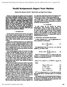
Figure 1: Network example where connectivity among nodes, represented by colored circles, is denoted by a line joining them.

municating nodes. Node j ∈ J only communicates with nodes in its one-hop neighborhood (ball) B j ⊆ J . The graph G is assumed connected, that is, any two nodes in G are connected by a (perhaps multihop) path in G . Notice that nodes do not have to be fully connected (any-to-any), and G is allowed to contain cycles. At every node j ∈ J , a labeled training set S j := {(x jn , y jn ) : n = 1, . . . , N j } of size N j is available, where x jn ∈ X is a p × 1 data vector belonging to the input space X ⊆ R p , and y jn ∈ Y := {−1, 1} denotes its corresponding class label.2 Given S j per node j, the goal is to find a maximum-margin linear discriminant function g(x) in a distributed fashion, and thus enable each node to classify any new input vector x to one of the two classes {−1, 1} without communicating S j to other nodes j′ 6= j. Potential application scenarios include but are not limited to the following ones. Example 1 (Wireless sensor networks). Consider a set of wireless sensors deployed to infer the presence or absence of a pollutant over a geographical area at any time tn . Sensor j measures and forms a local binary decision variable y jn ∈ {1, −1}, where y jn = 1(−1) indicates presence (absence) of the pollutant at the position vector x j := [x j1 , x j2 , x j3 ]T . (Each sensor knows its position x j using existing self-localization algorithms Langendoen and Reijers, 2003.) The goal is to have each low-cost sensor improve the performance of local detection achieved based on S j = {([xTj ,tn ]T , y jn ) : n = 1, . . . , N j }, and through collaboration with other sensors approach the global performance attainable if each sensor had available all other sensors data. Stringent power limitations prevent sensor j to send its set S j to all other sensors or to an FC, if the latter is available. If these sensors are acoustic and are deployed to classify underwater unmanned vehicles, divers or submarines, then low transmission bandwidth and multipath effects further discourage incremental communication of the local data sets to an FC (Akyildiz et al., 2005). Example 2 (Distributed medical databases). Suppose that S j are patient data records stored at a hospital j. Each x jn here contains patient descriptors (e.g., age, sex or blood pressure), and y jn is a particular diagnosis (e.g., the patient is diabetic or not). The objective is to automatically diagnose 2. Although not included in this model for simplicity, K-ary alphabets Y with K > 2 can be considered as well.

1666


(classify) a patient arriving at hospital j with descriptor x, using all available data {S j }Jj=1 , rather than S j alone. However, a nonchalant exchange of database entries (xTjn , y jn ) can pose a privacy risk for the information exchanged. Moreover, a large percentage of medical information may require exchanging high resolution images. Thus, communicating and processing large amounts of highdimensional medical data at an FC may be computationally prohibitive. Example 3 (Collaborative data mining). Consider two different government agencies, a local agency A and a nation-wide agency B, with corresponding databases SA and SB . Both agencies are willing to collaborate in order to classify jointly possible security threats. However, lower clearance level requirements at agency A prevents agency B from granting agency A open access to SB . Furthermore, even if an agreement granting temporary access to agency A were possible, databases SA and SB are confined to their current physical locations due to security policies. If {S j }Jj=1 were all centrally available at an FC, then the global variables w∗ and b∗ describing the centralized maximum-margin linear discriminant function g∗ (x) = xT w∗ + b∗ could be obtained by solving the convex optimization problem; see, for example, Schölkopf and Smola (2002, Ch. 7) N

j J 1 kwk2 +C ∑ ∑ ξ jn 2 j=1 n=1

{w∗ , b∗ } = arg min

w,b,{ξ jn }

s.t. y jn (wT x jn + b) ≥ 1 − ξ jn ∀ j ∈ J , n = 1, . . . , N j ξ jn ≥ 0

(1)

∀ j ∈ J , n = 1, . . . , N j

where the slack variables ξ jn account for non-linearly separable training sets, and C is a tunable positive scalar. Nonlinear discriminant functions g(x) can also be found along the lines of (1) after mapping vectors x jn to a higher dimensional space H ⊆ RP , with P > p, via a nonlinear transformation φ : X → H . The generalized maximum-margin linear classifier in H is then obtained after replacing x jn with φ(x jn ) in (1), and solving the following optimization problem N

j J 1 kwk2 +C ∑ ∑ ξ jn 2 j=1 n=1

{w∗ , b∗ } = arg min

w,b,{ξ jn }

s.t. y jn (wT φ(x jn ) + b) ≥ 1 − ξ jn ∀ j ∈ J , n = 1, . . . , N j ξ jn ≥ 0

(2)

∀ j ∈ J , n = 1, . . . , N j .

Problem (2) is typically tackled by solving its dual. Letting λ jn denote the Lagrange multiplier corresponding to the constraint y jn (wT φ(x jn ) + b) ≥ 1 − ξ jn , the dual problem of (2) is: max {λ jn }

− J

s.t.

1 2

J

J

Nj

Ni

∑∑∑ ∑

j=1 i=1 n=1 m=1

J

λ jn λim y jn yim φT (x jn )φ(xim ) + ∑

Nj

∑ λ jn

j=1 n=1

Nj

∑ ∑ λ jn y jn = 0

(3)

j=1 n=1

0 ≤ λ jn ≤ C

∀ j ∈ J , n = 1, . . . , N j . 1667


Using the Lagrange multipliers λ∗jn optimizing (3), and the Karush-Kuhn-Tucker (KKT) optimality conditions, the optimal classifier parameters can be expressed as J

w∗ = ∑

Nj

∑ λ∗jn y jn φ(x jn ),

j=1 n=1

b =y jn − w∗T φ(x jn ) ∗

(4)

with x jn in (4) satisfying λ∗jn ∈ (0,C). Training vectors corresponding to non-zero λ∗jn ’s constitute the SVs. Once the SVs are identified, all other training vectors with λ∗jn = 0 can be discarded since they do not contribute to w∗ . From this vantage point, SVs are the most informative elements of the training set. Solving (3) does not require knowledge of φ but only inner product values φT (x jn )φ(xim ) := K(x jn , xim ), which can be computed through a pre-selected positive semi-definite kernel K : X × X → R; see, for example, Schölkopf and Smola (2002, Ch. 2). Although not explicitly given, the optimal slack variables ξ∗jn can be found through the KKT conditions of (2) in terms of λ∗jn (Schölkopf and Smola, 2002). The optimal discriminant function can be also expressed in terms of kernels as g∗ (x) =

J

Nj

∑ ∑ λ∗jn y jn K(x jn , x) + b∗

(5)

j=1 n=1

i λ∗im yim K(xim , x jn ) for any SV x jn with λ∗jn ∈ (0,C). This so-called where b∗ = y jn − ∑Ji=1 ∑Nm=1 kernel trick allows finding maximum-margin linear classifiers in higher dimensional spaces without explicitly operating in such spaces (Schölkopf and Smola, 2002). The objective here is to develop fully distributed solvers of the centralized problems in (1) and (2) while guaranteeing performance approaching that of a centralized equivalent SVM. Although incremental solvers are possible, the size of information exchanges required might be excessive, especially if the number of SVs per node is large (Flouri et al., 2008; Lu et al., 2008). Recall that exchanging all local SVs among all nodes in the network several times is necessary for incremental DSVMs to approach the optimal centralized solution. Moreover, incremental schemes require a Hamiltonian cycle in the network to be identified in order to minimize the communication overhead. Computing such a cycle is an NP-hard task and in most cases a sub-optimal cycle is used at the expense of increased communication overhead. In other situations, communicating SVs directly might be prohibited because of the sensitivity of the information bore, as already mentioned in Examples 2 and 3.

3. Distributed Linear Support Vector Machine This section presents a reformulation of the maximum-margin linear classifier problem in (1) to an equivalent distributed form, which can be solved using the alternating direction method of multipliers (ADMoM) outlined in Appendix A. (For detailed exposition of the ADMoM, see, for example, Bertsekas and Tsitsiklis, 1997.) To this end, consider replacing the common (coupling) variables (w, b) in (1) with auxiliary per-node variables {(w j , b j )}Jj=1 , and adding consensus constraints to force these variables to agree across neighboring nodes. With proper scaling of the cost by J, the proposed consensus-based 1668


reformulation of (1) becomes 1 2

min

{w j ,b j ,ξ jn }

J

2

w + JC ∑ ∑ j J

Nj

∑ ξ jn

j=1 n=1

j=1

s.t. y jn (wTj x jn + b j ) ≥ 1 − ξ jn ξ jn ≥ 0

∀ j ∈ J , n = 1, . . . , N j

(6)

∀ j ∈ J , n = 1, . . . , N j ∀ j ∈ J , i ∈ B j.

w j = wi , b j = bi

From a high-level view, problem (6) can be solved in a distributed fashion because each node j can optimize only the j-dependent terms of the cost, and also meet all the consensus constraints w j = wi , b j = bi , by exchanging messages only with nodes i in its neighborhood B j . What is more, network connectivity ensures that consensus in neighborhoods enables network-wide consensus. And thus, as the ensuing lemma asserts, solving (6) is equivalent to solving (1) so long as the network remains connected. Lemma 1 If {(w j , b j )}Jj=1 denotes a feasible solution of (6), and the graph G is connected, then problems (1) and (6) are equivalent, that is, w j = w and b j = b ∀ j = 1, . . . , J, where (w, b) is a feasible solution of (1). Proof See Appendix B. To specify how (6) can be solved using the ADMoM, define for notational brevity the augmented vector v j := [wTj , b j ]T , the augmented matrix X j := [[x j1 , . . . , x jN j ]T , 1 j ], the diagonal label matrix Y j := diag([y j1 , . . . , y jN j ]), and the vector of slack variables ξ j := [ξ j1 , . . . , ξ jN j ]T . With these definitions, it follows readily that w j = (I p+1 − Π p+1 )v j , where Π p+1 is a (p + 1) × (p + 1) matrix with zeros everywhere except for the (p + 1, p + 1)-st entry, given by [Π p+1 ](p+1)(p+1) = 1. Thus, problem (6) can be rewritten as min

{v j ,ξ j ,ω ji }

1 2

J

J

j=1

j=1

∑ vTj (I p+1 − Π p+1 )v j +JC ∑ 1Tj ξ j

s.t. Y j X j v j 1 j − ξ j

∀j ∈ J

ξj 0j

∀j ∈ J

v j = ω ji , ω ji = vi

∀ j ∈ J , ∀i ∈ B j

(7)

where the redundant variables {ω ji } will turn out to facilitate the decoupling of the classifier parameters v j at node j from those of their neighbors at neighbors i ∈ B j . As in the centralized case, problem (7) will be solved through its dual. Toward this objective, let α ji1 (α ji2 ) denote the Lagrange multipliers corresponding to the constraint v j = ω ji (respectively ω ji = vi ), and consider what we term surrogate augmented Lagrangian function

L ({v j }, {ξ j }, {ω ji },{α jik }) = J

+∑

J J 1 J T T 1 ξ + v (I −Π )v +JC ∑ j p+1 p+1 j ∑ j j ∑ ∑ αTji1 (v j −ω ji ) 2 j=1 j=1 i∈B j j=1

η

J

2 η J

2 + ∑ ∑ ω ji −vi 2 j=1 i∈B j

∑ αTji2 (ω ji −vi )+ 2 ∑ ∑ v j −ω ji

j=1 i∈B j

j=1 i∈B j

1669

(8)


where the adjective “surrogate” is used because L does not include the set of constraints W := {Y j X j v j 1 j − ξ j , ξ j 0 j }, and the adjective “augmented” because L includes two quadratic terms (scaled by the tuning constant η > 0) to further regularize the equality constraints in (7). The role of these quadratic terms ||v j − ω ji ||2 and ||ω ji − vi ||2 is twofold: (a) they effect strict convexity of L with respect to (w.r.t.) ω ji , and thus ensure convergence to the unique optimum of the global cost (whenever possible), even when the local costs are convex but not strictly so; and (b) through the scalar η, they allow one to trade off speed of convergence for steady-state approximation error (Bertsekas and Tsitsiklis, 1997, Ch. 3). Consider now solving (7) iteratively by minimizing L in a cyclic fashion with respect to one set of variables while keeping all other variables fixed. The multipliers {α ji1 , α ji2 } must be also updated per iteration using gradient ascent. The iterations required per node j are summarized in the following lemma.

Lemma 2 The distributed iterations solving (7) are {v j (t+1), ξ j (t+1)} = arg

min

{v j ,ξ j }∈W

L ({v j }, {ξ j }, {ω ji (t)}, {α jik (t)}),

{ω ji (t+1)} = arg min L ({v j (t+1)}, {ξ j (t+1)}, {ω ji }, {α jik (t)}), {ω ji }

(9) (10)

α ji1 (t+1) = α ji1 (t) + η(v j (t+1) − ω ji (t+1))

∀ j ∈ J , ∀i ∈ B j ,

(11)

α ji2 (t+1) = α ji2 (t) + η(ω ji (t+1) − vi (t+1))

∀ j ∈ J , ∀i ∈ B j .

(12)

and correspond to the ADMoM solver reviewed in Appendix A. Proof See Appendix C. Lemma 2 links the proposed DSVM design with the convergent ADMoM solver, and thus ensures convergence of the novel MoM-DSVM to the centralized SVM classifier. However, for the particular problem at hand it is possible to simplify iterations (9)-(12). Indeed, simple inspection of (8) confirms that with all other variables fixed, the cost in (10) is linear-quadratic in ω ji ; hence, ω ji (t + 1) can be found in closed form per iteration, and the resulting closed-form expression can be substituted back to eliminate ω ji from L . Furthermore, Appendix D shows that the two sets of multipliers α ji1 and α ji2 can be combined into one set α j after appropriate initialization of the iterations (11) and (12), as asserted by the following lemma. Lemma 3 Selecting α ji1 (0) = α ji2 (0) = 0(p+1)×1 as initialization ∀ j ∈ J , ∀i ∈ B j , iterations (9)(12) reduce to {v j (t+1), ξ j (t+1)} = arg

min

{v j ,ξ j }∈W

α j (t + 1) = α j (t) +

L ′ ({v j }, {ξ j }, {v j (t)}, {α j (t)}),

η [v j (t + 1) − vi (t + 1)] ∀ j ∈ J 2 i∈∑ Bj

1670

(13) (14)


where α j (t) := ∑i∈B j α ji1 (t), and L ′ is given by

L ′ ({v j }, {ξ j }, {v j (t)}, {α j (t)}) =

1 2

J

J

∑ vTj (I p+1 − Π p+1 )v j + JC ∑ 1Tj ξ j j=1

j=1

2

1 T

+ 2 ∑ α j (t)v j + η ∑ ∑

v j − 2 [v j (t) + vi (t)] . j=1 i∈B j j=1 J

J

Proof See Appendix D.

(15)

The optimization problem in (13) involves the reduced Lagrangian L ′ in (15), which is linearquadratic in v j and ξ j . In addition, the constraint set W is linear in these variables. To solve this constrained minimization problem through its dual, let λ j := [λ j1 , . . . , λ jN j ]T denote Lagrange multipliers per node corresponding to the constraints Y j X j v j 1 j − ξ j . Solving the dual of (13) yields the optimal λ j at iteration t + 1, namely λ j (t + 1), as a function of v j (t) and α j (t); while the KKT conditions provide expressions for v j (t + 1) as a function of α j (t), and the optimal dual variables λ j (t + 1). Notwithstanding, the resultant iterations are decoupled across nodes. These iterations and the associated convergence guarantees can be summarized as follows. Proposition 1 Consider the per node iterates λ j (t), v j (t) and α j (t), given by T 1 −1 T − λTj Y j X j U−1 λ j, j X j Y j λ j + 1 j + Y j X j U j f j (t) λ j : 0 j λ j JC1 j 2 T X j Y j λ j (t + 1) − f j (t) , v j (t + 1) = U−1 j η α j (t + 1) = α j (t) + ∑ [v j (t + 1) − vi (t + 1)] 2 i∈B j λ j (t + 1) = arg

max

(16) (17) (18)

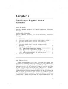
where U j := (1 + 2η|B j |)I p+1 − Π p+1 , f j (t) := 2α j (t) − η ∑i∈B j [v j (t) + vi (t)], η > 0, and arbitrary initialization vectors λ j (0), v j (0), and α j (0) = 0(p+1)×1 . The iterate v j (t) converges to the solution of (7), call it v∗ , as t → ∞; that is, limt→∞ v j (t) = v∗ . Proof See Appendix E. Similar to the centralized SVM algorithm, if [λ j (t)]n 6= 0, then [xTjn , 1]T is an SV. Finding λ j (t + 1) as in (16) requires solving a quadratic optimization problem similar to the one that a centralized SVM would solve, for example, via a gradient projection algorithm or an interior point method; see for example, Schölkopf and Smola (2002, Ch. 6). However, the number of variables involved in (16) per iteration per node is considerably smaller when compared to its centralized counterpart, namely N j versus ∑Jj=1 N j . Also, the optimal local slack variables ξ∗j can be found via the KKT conditions for (13). The ADMoM-based DSVM (MoM-DSVM) iterations (16)-(18) are summarized as Algorithm 1, and are illustrated in Figure 2. All nodes have available JC and η. Also, every node computes T its local N j × N j matrix Y j X j U−1 j X j Y j , which remains unchanged throughout the entire algorithm. Every node then updates its local (p + 1) × 1 estimates v j (t) and α j (t); and the N j × 1 vector λ j (t). 1671


At iteration t + 1, node j computes vector f j (t) locally to obtain its local λ j (t + 1) via (16). Vector λ j (t + 1) together with the local training set S j are used at node j to compute v j (t + 1) via (17). Next, node j broadcasts its newly updated local estimates v j (t + 1) to all its one-hop neighbors i ∈ B j . Iteration t + 1 resumes when every node updates its local α j (t + 1) vector via (18). Note that at any given iteration t of the algorithm, each node j can evaluate its own local discriminant (t) function g j (x) for any vector x ∈ X as (t)

g j (x) = [xT , 1]v j (t)

(19)

which from Proposition 1 is guaranteed to converge to the same solution across all nodes as t → ∞. Simulated tests in Section 5 will demonstrate that after a few iterations the classification performance of (19) outperforms that of the local discriminant function obtained based on the local training set alone. The effect of η on the convergence rate of MoM-DSVM will be tested numerically in Section 5.

Figure 2: Visualization of iterations (16)-(18): (left) every node j ∈ J computes λ j (t + 1) to obtain v j (t + 1), and then broadcasts v j (t + 1) to all neighbors i ∈ B j ; (right) once every node j ∈ J has received vi (t + 1) from all i ∈ B j , it computes α j (t + 1).

Remark 1 The messages exchanged among neighboring nodes in the MoM-DSVM algorithm correspond to local estimates v j (t), which together with the local multiplier vectors α j (t), convey sufficient information about the local training sets to achieve consensus globally. Per iteration and per node a message of fixed size (p + 1) × 1 is broadcasted (vectors α j are not exchanged among nodes.) This is to be contrasted with incremental DSVM algorithms in, for example, Lu et al. (2008), Flouri et al. (2006) and Flouri et al. (2008), where the size of the messages exchanged between neighboring nodes depends on the number of SVs found at each incremental step. Although the SVs of each training set may be few, the overall number of SVs may remain large, thus consuming considerable power when transmitting SVs from one node to the next. Remark 2 Real networks are prone to node failures, for example, sensors in a WSN may run out of battery during operation. Thanks to its fully decentralized mode of operation, the novel MoM-DSVM algorithm guarantees that the remaining nodes in the network will reach consensus as long as the 1672


Algorithm 1 MoM-DSVM Require: Randomly initialize v j (0), and α j (0) = 0(p+1)×1 for every j ∈ J 1: for t = 0, 1, 2, . . . do 2: for all j ∈ J do 3: Compute λ j (t + 1) via (16). 4: Compute v j (t + 1) via (17). 5: end for 6: for all j ∈ J do 7: Broadcast v j (t + 1) to all neighbors i ∈ B j . 8: end for 9: for all j ∈ J do 10: Compute α j (t + 1) via (18). 11: end for 12: end for node that fails, say jo ∈ J , does not correspond to a cut-vertex of G . In this case, the operational network graph Go := G − jo remains connected, and thus surviving nodes can percolate information throughout Go . Of course, S jo will not participate in training the SVM. If jo is a cut-vertex of G , the algorithm will remain operational in each connected component of the resulting sub-graph Go , reaching consensus among nodes in each of the connected components. 3.1 Online Distributed Support Vector Machine In many distributed learning tasks data arrive sequentially, and possibly asynchronously. In addition, the processes to be learned may change with time. In such cases, training examples need to be added or removed from each local training set S j . Training sets of increasing of decreasing size can be expressed in terms of time-varying augmented data matrices X j (t), and corresponding label matrices Y j (t). An online version of DSVM is thus well motivated when a new training example x jn (t) along with its label y jn (t) acquired at time t are incorporated into X j (t) and Y j (t), respectively. The corresponding modified iterations are given by (cf. (16)-(18)) λ j (t + 1) = arg

max

1 T − λTj Y j (t + 1)X j (t + 1)U−1 j X j (t + 1) Y j (t + 1)λ j 2 T λ j, (20) + 1 j − Y j (t + 1)X j (t + 1)U−1 f (t) j j !

λ j : 0 j (t+1)λ j JC1 j (t+1)

v j (t + 1) = U−1 X j (t + 1)T Y j (t + 1)λ j (t + 1) − 2α j (t) + η ∑ [v j (t) + vi (t)] , j α j (t + 1) = α j (t) +

η [v j (t + 1) − vi (t + 1)]. 2 i∈∑ Bj

(21)

i∈B j

(22)

Note that the dimensionality of λ j must vary to accommodate the variable number of S j elements at every time instant t. The online MoM-DSVM classifier is summarized as Algorithm 2. For this algorithm to run, no conditions need to be imposed on how the sets S j (t) increase or decrease. Their changes can be asynchronous and may comprise multiple training examples at once. In principle, 1673


Algorithm 2 Online MoM-DSVM Require: Randomly initialize v j (0), and α j (0) = 0(p+1)×1 for every j ∈ J . 1: for t = 0, 1, 2, . . . do 2: for all j ∈ J do T 3: Update Y j (t + 1)X j (t + 1)U−1 j X j (t + 1) Y j (t + 1). 4: Compute λ j (t + 1) via (20). 5: Compute v j (t + 1) via (21). 6: end for 7: for all j ∈ J do 8: Broadcast v j (t + 1) to all neighbors i ∈ B j . 9: end for 10: for all j ∈ J do 11: Compute α j (t + 1) via (22). 12: end for 13: end for the parameters η and C can also become time-dependent. The effect of these parameters will be discussed in Section 5. Intuitively speaking, if the training sets remain invariant across a sufficient number of time instants, v j (t) will closely track the optimal linear classifier. Rigorous convergence analysis of Algorithm 2 for any given rate of change of the training set goes beyond the scope of this work. Simulations will however demonstrate that the modified iterations in (20)-(22) are able to track changes in the training sets even when these occur at every time instant t.

Remark 3 Compared to existing centralized online SVM alternatives in, for example, Cauwenberghs and Poggio (2000) and Fung and Mangasarian (2002), the online MoM-DSVM algorithm of this section allows seamless integration of both distributed and online processing. Nodes with training sets available at initialization and nodes that are acquiring their training sets online can be integrated to jointly find the maximum-margin linear classifier. Furthermore, whenever needed, the online MoM-DSVM can return a partially trained model constructed with examples available to the network at any given time. Likewise, elements of the training sets can be removed without having to restart the MoM-DSVM algorithm. This feature also allows adapting MoM-DSVM to jointly operate with algorithms that account for concept drift (Klinkenberg and Joachims, 2000). In the classification context, concept drift defines a change in the true classification boundaries between classes. In general, accounting for concept drift requires two main steps, which can be easily handled by the online MoM-DSVM: (i) acquisition of updated elements in the training set that better describe the current concept; and (ii) removal of outdated elements from the training set.

4. Distributed Nonlinear Support Vector Machine In Section 3, problem (1) was reformulated to allow all nodes to consent on v∗ . However, applying an identical reformulation to the nonlinear classification problem in (2) would require updates in 1674


(16)-(18) to be carried in H . As the dimensionality P of H increases, the local computation and communication complexities become increasingly prohibitive. Our approach to mitigate this well-known “curse of dimensionality” is to enforce consensus of the local discriminants g∗j on a subspace of reduced rank L < P. To this end, we project the consensus constraints corresponding to (2) and consider the optimization problem (cf. (6)) 1 2

min

{w j ,b j ,ξ j }

J

J

j=1

j=1

∑ kw j k2 + JC ∑ 1Tj ξ j

s.t. Y j (Φ(X j )w j + 1 j b j ) 1 j − ξ j ∀ j ∈ J ξj 0j

∀j ∈ J

Gw j = Gwi

∀ j ∈ J ,i ∈ Bj

b j = bi

∀ j ∈ J ,i ∈ Bj

(23)

where Φ(X j ) := [φ(x j1 ), . . . , φ(x jN j )]T , and G := [φ(χ1 ), . . . , φ(χL )]T is a fat L × P matrix common to all nodes with preselected vectors {χl }Ll=1 specifying its rows. Each χl ∈ X corresponds to a φ(χl ) ∈ H , which at the optimal solution {w∗j , b∗j }Jj=1 of (23), satisfies φT (χl )w∗1 = · · · = φT (χl )w∗J = φT (χl )w∗ . The projected constraints {Gw j = Gwi } along with {b j = bi } force all nodes to agree on the value of the local discriminant functions g∗j (χl ) at the vectors {χl }Ll=1 , but not necessarily for all x ∈ X . This is the price paid for reducing the computational complexity of (23) to an affordable level. Clearly, the choice of vectors {χl }Ll=1 , their number L, and the local training sets S j determine how similar the local discriminant functions g∗j are. If G = IP , then (23) reduces to (6), and g∗1 (x) = . . . = g∗J (x) = g∗ (x), ∀x ∈ X , but the high dimensionality challenge appears. At the end of this section, we will provide different design choices for {χl }Ll=1 , and test them via simulations in Section 5. Because the cost in (23) is strictly convex w.r.t. w j , it guarantees that the set of optimal vectors {w∗j } is unique even when G is a ‘fat’ matrix (L < P) and/or ill-conditioned (Bertsekas, 1999, Prop. 5.2.1). As in (2), having {w∗j } known is of limited use, since the mapping φ may be unknown, or if known, evaluating vectors φ(x) may entail an excessive computational cost. Fortunately, the resulting discriminant function g∗j (x) admits a reduced-complexity solution because it can be expressed in terms of kernels, as shown by the following theorem. Theorem 4 For every positive semi-definite kernel K(·, ·), the discriminant functions g∗j (x) = φT (x)w∗j + b∗j with {w∗j , b∗j } denoting the optimal solution of (23), can be written as g∗j (x)

=

Nj

L

n=1

l=1

∑ a∗jn K(x, x jn ) + ∑ c∗jl K(x, χl ) + b∗j , ∀ j ∈ J

(24)

where {a∗jn } and {c∗jl } are real-valued scalar coefficients. Proof See Appendix F. The space of functions g j described by (24) is fully determined by the span of the kernel function K(·, ·) centered at training vectors {x jn , n = 1, . . . , N j } per node, and also at the vectors {χl }Ll=1 which are common to all nodes. Thus, similarity of the discriminant functions g∗j across nodes is 1675


naturally constrained by the corresponding S j . Theorem 1 also reveals the effect of {χl }Ll=1 on the {g∗j }. By introducing vectors {χl }Ll=1 common to all nodes, a subset of basis functions common to all local functional spaces is introduced a fortiori. Coefficients a∗jn and c∗jl are found so that all local discriminants g∗j agree on their values at points {χl }Ll=1 . Intuitively, at every node these coefficients summarize the global information available to the network. Theorem 1 is an existence result whereby each nonlinear discriminant function g∗j is expressible in terms of S j and {χl }Ll=1 . However, finding the coefficients a∗jn , c∗jl and b∗j in a distributed fashion remains an issue. Next, it is shown that these coefficients can be obtained iteratively by applying the ADMoM solver to (23). Similar to (7), introduce auxiliary variables {ω ji } ({ζ ji }) to decouple the constraints Gw j = Gwi (b j = bi ) across nodes, and α jik (β jik ) denote the corresponding Lagrange multipliers (cf. (8)). The surrogate augmented Lagrangian for problem (23) is then

L ({w j },{ξ j },{ω ji },{α jik },{ζ ji },{β jik }) = J

+∑

j=1 i∈B j

+

J

∑ αTji2 (ω ji −Gwi )+ ∑

J J 1 J T 2 1 ξ + kw k +JC ∑ j j ∑ ∑ αTji1 (Gw j −ω ji ) ∑ j 2 j=1 j=1 i∈B j j=1 J

∑ β ji1 (b j −ζ ji )+ ∑

∑ β ji2 (ζ ji −bi )

j=1 i∈B j

j=1 i∈B j

J J J

η J

Gw j −ω ji 2 + η ∑ ∑ ω ji −Gwi 2 + η ∑ ∑ b j −ζ ji 2 + η ∑ ∑ ζ ji −bi 2 . ∑ ∑ 2 j=1 i∈B j 2 j=1 i∈B j 2 j=1 i∈B j 2 j=1 i∈B j

Following the steps of Lemma 2, and with {α jik } and {β jik } initialized at zero, the ADMoM iterations take the form {w j (t+1), b j (t+1), ξ j (t+1)} = arg

min L ′({w j }, {b j }, {ξ j }, {α j (t)}, {β j (t)}),

{w j,b j,ξ j}∈W

α j (t+1) = α j (t) + β j (t+1) = β j (t) +

η G[w j (t + 1) − wi (t + 1)], 2 i∈∑ Bj

η [b j (t + 1) − bi (t + 1)] 2 i∈∑ Bj

(25) (26) (27)

where L ′ is defined similar to (8), α j (t) as in Lemma 3, and β j (t) := ∑i∈B j β ji1 (t). The ADMoM iterations (25)-(27) will not be explicitly solved since iterates w j (t) lie in the high-dimensional space H . Nevertheless, our objective is not to find w∗j , but rather the discriminant function g∗j (x). To this end, let Γ := [χ1 , . . . , χL ]T , and define the kernel matrices with entries [K(X j , X j )]n,m := K(x jn , x jm ),

(28)

[K(X j , Γ)]n,l := K(x jn , χl ),

(29)

[K(Γ, Γ)]l,l ′ := K(χl , χl ′ ).

(30)

(t)

From Theorem 1 it follows that each local update g j (x) = φT (x)w j (t) + b j (t) admits per iteration t a solution expressed in terms of kernels. The latter is specified by the coefficients {a jn (t)}, {c jl (t)} and {b j (t)} that can be obtained in closed form, as shown in the next proposition.

1676


Proposition 2 Let λ j := [λ j1 , . . . , λ jN j ]T denote the Lagrange multiplier corresponding to the con(t)

e j (t) := Gw j (t). The local discriminant function g j (x) straint Y j (Φ(X j )w j +1 j b j ) 1 j −ξ j , and w at iteration t is (t) g j (x)

=

Nj

L

n=1

l=1

∑ a jn (t)K(x, x jn) + ∑ c jl (t)K(x, χl ) + b j (t)

(31)

where a j (t) := [a j1 (t), . . . , a jN j (t)]T , c j (t) := [c j1 (t), . . . , c jL (t)]T , and b j (t) are given by a j (t) := Y j λ j (t), e −1 [K(Γ, Γ)f j (t) − K(Γ, X j )Y j λ j (t)] −ef j (t), c j (t) := 2η|B j |U j

b j (t) :=

1 2η|B j |

T 1 j Y j λ j (t) − h j (t)

(32) (33) (34)

e j := IL + 2η|B j |K(Γ, Γ), with λ j (t) denoting the vector multiplier update available at iteration t, U ef j (t) := 2α j (t) − η ∑i∈B [e e i (t)] and h j (t) := 2β j (t) − η ∑i∈B j [b j (t) + bi (t)]. w j (t) + w j Proof See Appendix G.

Proposition 2 asserts that in order to find a j (t), c j (t) and b j (t) in (32), (33) and (34), it suffices e j (t), b j (t), α j (t), and β j (t). Note that finding the L × 1 vector w e j (t) from w j (t) to obtain λ j (t), w e j (t), incurs complexity of order O(L). The next proposition shows how to iteratively update λ j (t), w b j (t), α j (t), and β j (t) in a distributed fashion. e j (t), b j (t), α j (t) and β j (t) can be obtained as Proposition 3 The iterates λ j (t), w

1 j 1Tj 1 T e − λ j Y j K(X j , X j ) − K(X j , X j ) + λ j (t + 1) = arg max Y j λ j + 1Tj λ j 2η|B j | λ j : 0 j λ j JC1 j 2 1T T e e − f j (t) K(Γ, X j )−K(Γ, X j ) + h j (t) Y jλ j, (35) 2η|B j | h i h i e X j ) Y j λ j (t + 1)− K(Γ, Γ)−K(Γ, e Γ) ef j (t), e j (t + 1) = K(Γ, X j ) − K(Γ, (36) w 1 T 1 j Y j λ j (t + 1) − h j (t) , 2η|B j | η e i (t + 1)], α j (t + 1) = α j (t) + ∑ [e w j (t + 1) − w 2 i∈B j b j (t + 1) =

β j (t + 1) = β j (t) +

η [b j (t + 1) − bi (t + 1)] 2 i∈∑ Bj

(37)

(38) (39)

e e −1 K(Γ, Z′ ). With arbitrary initialization λ j (0), w e j (0), and where K(Z, Z′ ) := 2η|B j |K(Z, Γ)U j b j (0); and α j (0) = 0L×1 and β j (0) = 0, the iterates {a jn (t)}, {c jl (t)} and {b j (t)} in (32), (33) and (34) converge to {a∗jn }, {c∗jl } and {b∗j } in (24), as t → ∞, ∀ j ∈ J , n = 1, . . . , N j , and l = 1, . . . , L. Proof See Appendix H.

1677


Algorithm 3 MoM-NDSVM e j (0) and b j (0); and α j (0) = 0L×1 and β j (0) = 0 for every j ∈ J . Require: Randomly initialize w 1: for t = 0, 1, 2, . . . do 2: for all j ∈ J do 3: Compute λ j (t + 1) via (35). e j (t + 1) via (36). 4: Compute w 5: Compute b j (t + 1) via (37). 6: end for 7: for all j ∈ J do e j (t + 1) and b j (t + 1) to all neighbors i ∈ B j . 8: Broadcast w 9: end for 10: for all j ∈ J do 11: Compute α j (t + 1) via (38). 12: Compute β j (t + 1) via (39). 13: Compute a j (t), c j (t) and b j (t) via (32), (33) and (34), respectively. 14: end for 15: end for

The iterations comprising the ADMoM-based non-linear DSVM (MoM-NDSVM) are summarized as Algorithm 3. It is important to stress that Algorithm 3 starts by having all nodes agree on the common quantities Γ, JC, η, and K(·, ·). Also, each node computes its local kernel matrices as in (28)-(30), which remain unchanged throughout. Subsequently, Algorithm 3 runs in a manner analogous to Algorithm 1, with the difference that every node communicates an (L + 1) × 1 vector e j (t) and b j (t). (instead of (p + 1) × 1) for its neighbors to receive w 4.1 On the Optimality of NDSVM and the Selection of Common Vectors

By construction, Algorithm 3 produces local discriminant functions whose predictions for {χl }Ll=1 are the same for all nodes in the network; that is, g∗1 (χl ) = . . . = g∗J (χl ) = g∗ (χl ) for l = 1, . . . , L, where g∗ (χl ) = φT (χl )w∗ + b∗ , and {w∗ , b∗ } are the optimal solution of the centralized problem (2). Viewing {χl }Ll=1 as a classification query, the proposed MoM-NDSVM algorithm can be implemented as follows. Having this query presented at any node j entailing a set of unlabeled vectors {χl }Ll=1 , the novel scheme first percolates {χl }Ll=1 throughout the network.3 Problem (23) is subsequently solved in a distributed fashion using Algorithm 3. Notice that in this procedure no database information is shared. Although optimal in the sense of being convergent to its centralized counterpart, the algorithm just described needs to be run for every new classification query. Alternatively, one can envision procedures to find discriminant functions in a distributed fashion that classify new queries without having to re-run the distributed algorithm. The key is to pre-select a fixed set {χl }Ll=1 for which g∗ in (5) is (approximately) equivalent to g∗j in (24) for all j ∈ J . From Theorem 1, we know that all local functions g∗j share a common space spanned by the χl -induced kernels {K(·, χl )}. If the space H where g∗ lies is finite dimensional, for example, when adopting linear or polynomial 3. Percolating {χ}Ll=1 in a distributed fashion through the network can be carried in a finite number of iterations at most equal to the diameter of the network.

1678


kernels in (5), one can always find a finite-size set {χl }Ll=1 such that the space spanned by the set of kernels {K(·, χl )} contains H , and thus g∗1 (x) = . . . = g∗J (x) = g∗ (x) ∀x ∈ X (Predd et al., 2006). Indeed, when using linear kernels, the MoM-NDSVM developed here boils down to the MoM-DSVM developed in Section 3 for a suitable finite-size set {χl }Ll=1 . In general, however, the space spanned by {K(·, χl )} may have lower dimensionality than H ; thus, local functions g∗j do not coincide at every point. In this case, MoM-NDSVM finds local approximations to the centralized g∗ which accommodate information available to all nodes. The degree of approximation depends on the choice of {χl }Ll=1 . In what follows, we describe two alternatives to constructing such a set {χl }Ll=1 . • Grid-based designs. Consider every entry k of the training vectors {x jn }, and form the intervals Ik := [xkmin , xkmax ], k = 1, . . . , p, where xkmin := min j∈J , n=1,...,N j [x jn ]k and xkmax := max j∈J , n=1,...,N j [x jn ]k . Take for convenience L = M p , and partition uniformly each Ik to obtain a set of M equidistant points Qk := {qk1 , . . . , qkM }. The set {χl }Ll=1 can be formed by taking all M p possible vectors with entries drawn from the Cartesian product Q1 × . . . , ×Q p . One possible set we use for generating the {χl }Ll=1 vectors is obtained by selecting the k-th entry of the l-th vector as [χl ]k = qk, l mod M+1 , where l = 1, . . . , M p and k = 1, . . . , p. In M k−1

this case, MoM-NDSVM performs a global consensus step on the entry-wise maxima and minima of the training vectors {x jn }. Global consensus on the entry-wise maxima and minima can be computed exactly in a finite number of iterations equal to at most the diameter of the graph G .

• Random designs. Once again, we consider every entry k of the training vectors {x jn }. MoMNDSVM starts by performing a consensus step on the entry-wise maxima and minima of the local training vectors {x jn }. The set {χl }Ll=1 is formed by drawing elements χl randomly from a uniform p-dimensional distribution with extreme points per entry given by the extreme points xkmin and xkmax , k = 1, . . . , p. To agree on the set {χl }Ll=1 , all nodes in the network are assumed to share a common seed used to initialize the random sampling algorithms. As mentioned earlier, the number of points L affects how close local functions are to each other as well as to the centralized one. The choice of L also depends on the kernel used, prior knowledge of the discriminant function, and the available local training data N j . Increasing L guarantees that local functions will be asymptotically close to each other regardless of N j ; however, the communication cost and computational complexity per node will increase according to L [cf. Algorithm 3]. On the other hand, a small L reduces the communication overhead at the price of increasing the disagreement among the g∗j ’s. This trade-off will be further explored in the ensuing section through simulated tests.

5. Numerical Simulations In this section, we analyze the performance of both MoM-DSVM and MoM-NDSVM algorithms using different networks with synthetic and real-world training sets. Although we focus on the binary classification case, it is worth remembering that K-ary classification problems with K > 2 can be solved via binary classification schemes, for example, by using one versus all classifiers, or all versus all classifiers (Duda et al., 2002, Ch. 5). 1679


5.1 Linear Classifiers In this section, we present experiments on synthetic and real data to illustrate the performance of our distributed method for training linear SVMs. 5.1.1 T EST C ASE 1: S YNTHETIC T RAINING S ET Consider a randomly generated network with J = 30 nodes. The network is connected with algebraic connectivity 0.0448 and average degree per node 3.267. Each node acquires labeled training examples from two different classes C1 and C2 with corresponding labels y1 = 1 and y2 = −1. Classes C1 and C2 are equiprobable and consist of random vectors drawn from a two-dimensional Gaussian distribution with common covariance matrix Σ = [1, 0; 0, 2], and mean vectors m1 = [−1, −1]T and m2 = [1, 1]T , respectively. Each local training set S j consists of N j = N = 10 labeled examples and was generated by: (i) randomly choosing class Ck , k = 1, 2; and, (ii) randomly generating a labeled example (xTjn , y jn = Ck ) with x jn ∼ N (mk , Σ). Thus, the global training set contains JN = 300 training examples. Likewise, a test set STest := {(e xn , yen ), n = 1, . . . , NT } with NT = 600 examples, drawn as in (i) and (ii), is used to evaluate the generalization performance of the classifiers. The Bayes optimal classifier for this 2-class problem is linear (Duda et al., 2002, Ch. 2), with risk RBayes = 0.1103. The empirical risk of the centralized SVM in (1) is defined as Rcentral emp :=

1 NT

NT

1

∑ 2 |eyn − yˆn |

n=1

where yˆn is the predicted label for e xn . The average empirical risk of the MoM-DSVM algorithm as a function of the number of iterations is defined as Remp (t) :=

J

1 JNT

NT

1

∑ ∑ 2 |eyn − yˆ jn (t)|

(40)

j=1 n=1

where yˆ jn (t) is the label prediction at iteration t and node j for e xn , n = 1, . . . , NT using the SVM parameters in v j (t). The average empirical risk of the local SVMs across nodes Rlocal emp is defined as in (40) with yˆ jn found using only locally-trained SVMs. Figure 3 (left) depicts the risk of the MoM-DSVM algorithm as a function of the number of iterations t for different values of JC. In this test, η = 10 and a total of 500 Monte Carlo runs are performed with randomly drawn local training and test sets per run. The centralized and local empirical risks with C = 10 are included for comparison. The average local prediction performance is also evaluated. Clearly, the risk of the MoM-DSVM algorithm reduces as the number of iterations increases, quickly outperforming local-based predictions and approaching that of the centralized benchmark. To further visualize this test case, Figure 3 (right) shows the global training set, along with the linear discriminant functions found by the centralized SVM and the MoM-DSVM at two different nodes after 400 iterations with JC = 20 and η = 10. Local SVM results for two different nodes are also included for comparison. 5.1.2 T EST C ASE 2: MNIST T RAINING S ET Here, the MoM-DSVM is tested on the MNIST database of handwritten images (Lecun et al., 1998). The MNIST database contains images of digits 0 to 9. All images are of size 28 by 28 pixels. We consider the binary problem of classifying digit 2 versus digit 9 using a linear classifier. For this 1680


Figure 3: Evolution of the test error (RTest ) and prediction error (RPred ) of MoM-DSVM for a twoclass problem using synthetic data and a network with J = 30 nodes. Centralized SVM performance and average local SVMs performance are also plot for comparison (left). Decision boundary comparison among MoM-DSVM, centralized SVM and local SVM results for synthetic data generated from two Gaussian classes (right).

experiment each image is vectorized to a 784 by 1 vector. In particular, we take 5,900 training samples per digit, and a test set of 1,000 samples per digit. Both training and test sets used are as given by the MNIST database, that is, there is no preprocessing of the data. For simulations, we consider two randomly generated networks with J = 25, algebraic connectivity 3.2425, and average degree per node 12.80; and J = 50 nodes, algebraic connectivity 1.3961, and average degree per node 15.92. The training set is equally partitioned across nodes, thus every node in the network with J = 25 has N j = 472 training vectors, and every node in the network with J = 50 has N j = 236 samples. The distribution of samples across nodes influences the training phase of MoM-DSVM. For example, if data per node are biased toward one particular class, then the training phase may require more iterations to percolate appropriate information across the network. In the simulations, we consider the two extreme cases: (i) training data are evenly distributed across nodes, that is, every node has the same number of examples from digit 2 and from digit 9; and, (ii) highly biased local data, that is, every node has data corresponding to a single digit; thus, a local binary classifier cannot be constructed. The figures in this section correspond to one run of the MoM-DSVM for a network with noiseless communication links. Figure 4 shows the evolution of the test error for the network with 25 nodes and highly biased local data. Likewise, Figure 5 shows the evolution of the test error for the network with 50 nodes and highly biased local data. Different values for the penalties JC and η were used to illustrate their effect on both the classification performance and the convergence rate of MoM-DSVM. The parameter JC controls the final performance of the classifier; but for a finite number of iterations, η also influences the final performance of the classifier. Larger values of η may be desirable; however, if η is too large, the algorithm first focuses on reaching consensus across nodes disregarding the classification performance. Although, MoM-DSVM is guaranteed to converge for all η, a very large choice for η may hinder the convergence rate. 1681


Figure 4: Evolution of the test error (RTest ) of MoM-DSVM, with penalty coefficients JC = 1 (left) and JC = 5 (right), for a two-class problem using digits 2 and 9 from the MNIST data set unevenly distributed across nodes, and a network with J = 25 nodes.

Figure 5: Evolution of the test error (RTest ) of MoM-DSVM, with penalty coefficients JC = 1 (left) and JC = 5 (right), for a two-class problem using digits 2 and 9 from the MNIST data set unevenly distributed across nodes, and a network with J = 50 nodes.

Next, the dispersion of the solutions after 3,000 iterations for different values of η is tested. For our experiment, dispersion refers to how similar are the local v j (t) at every node. The meansquared error (MSE) of the solution across nodes is defined as ∆(t) := 1J ∑Jj=1 ||v j (t) − v¯ (t)||2 where v¯ (t) := 1J ∑Jj=1 v j (t). Table 1 shows ∆(t) at t = 3, 000 for different values of η and JC. Note that larger values of η lead to smaller dispersion in the solution; however, as illustrated in Figure 5, they do not imply faster convergence rates. 1682


∆(t) at t = 3, 000 η 1 5 10

J = 25 JC = 1 JC = 5 −7 3.1849×10 3.1870 × 10−7 −8 1.5591×10 1.4760 × 10−8 −10 2.9280×10 2.9112 × 10−10

J = 50 JC = 1 JC = 5 −7 2.3749 × 10 2.3227 × 10−7 −8 2.6613×10 2.6646×10−8 −9 3.6028×10 3.6207×10−9

Table 1: MSE ∆(t) with MNIST data set and biased local data for different values of η and JC.

Consider next data that are evenly distributed across nodes. The MNIST training set is partitioned across nodes ensuring that every node has an equal number of examples from digit 2 and digit 9. Figure 6 shows the evolution of the test error for the network with J = 25 nodes and Figure 7 shows the evolution of the test error for the network with J = 50 nodes for different values for the penalties JC and η. In this case, local classifiers achieve low test error after one iteration of the MoM-DSVM. In subsequent iterations MoM-DSVM forces all local classifiers to consent, but the test error does not decrease monotonically across iterations. This variation is small, ranging between 0.015 and 0.02, since all local classifiers already have low test error. Both Figures 6 and 7 show that between iterations 500 and 2, 000, the global test reaches a minimum value, then it increases and converges to a larger value. This non-monotonic behavior can be attributed to the fact that the MoM-DSVM iterates are not guaranteed to be monotonic. Moreover, before consensus is reached across all nodes the test error at any given node and iteration index does not necessarily need to be greater than the centralized one. It is also worth noticing the resemblance of the curves in the left and right panels of Figures 4, 5, 6 and 7. Although the test error is nearly identical for JC = 1 and JC = 5, this does not imply that the v j (t) are nearly identical across iterations. Furthermore, the insensitivity w.r.t. small changes in JC reveals that in order to affect the classifier performance, the parameter JC must vary in the order of J. Relating the distributed setting with its centralized counterpart, it follows that with, for example, J = 25 a change in JC from 1 to 5 in the distributed setup of (6), corresponds to a change in C from 0.04 to 0.20 for the centralized setting of (1). Such a small change in C explains why the classification performance of the equivalent centralized scenarios is nearly identical as reflected in the figures. In both biased and evenly distributed data, after a few iterations, MoM-DSVM yields an average performance close to the optimal one. It is also interesting to note that in the biased data case, nodes alone cannot construct an approximate classifier since they do not have samples from both classes. If an incremental approach were used it would need at least one full cycle through the network to enable construction of local estimators per node. Finally, the effect of network connectivity on the performance of MoM-DSVM is explored. In this experiment, we consider a network with J = 25 nodes, ring topology and biased data distribution as before. The performance of MoM-DSVM is illustrated by Figure 8. It is clear that in this case a larger η improves the convergence rate. Also, note that after a few iterations the average performance of the classifier across the network is close to the optimal. In practice, a small reduction of performance over the centralized classifier may be acceptable in which case MoM-DSVM can stop after a small number of iterations. Note that the communication cost of MoM-DSVM can be easily computed at any iteration in terms of the number of scalars transmitted across the network. 1683


Figure 6: Evolution of the test error (RTest ) of MoM-DSVM, with penalty coefficients JC = 1 (left) and JC = 5 (right), for a two-class problem using digits 2 and 9 from the MNIST data set evenly distributed across nodes, and a network with J = 25 nodes.

Figure 7: Evolution of the test error (RTest ) of MoM-DSVM, with penalty coefficients JC = 1 (left) and JC = 5 (right), for a two-class problem using digits 2 and 9 from the MNIST data set evenly distributed across nodes, and a network with J = 50 nodes.

For the MNIST data set, the total communication cost up to iteration t is 785Jt scalars (cf. Section 3). 5.1.3 T EST C ASE 3: S EQUENTIAL O PERATION Consider a network with J = 10 nodes, algebraic connectivity 0.3267, and average degree per node 2.80. Data from two classes arrive sequentially at each node in the following fashion: at t = 0 each node has available one labeled training example drawn from the class distributions C1 and C2 1684


Figure 8: Evolution of the test error (RTest ) of MoM-DSVM, with penalty coefficients JC = 1, for a two-class problem using digits 2 and 9 from the MNIST data set unevenly distributed across nodes, and a network with ring topology and J = 25 nodes.

described in Test Case 1. From t = 0 to t = 19, each node acquires a new labeled training example per iteration from this same distribution. From t = 20 to t = 99, no new training example is acquired. After iteration t = 99, the distribution from which training examples in class C1 were generated changes to a two-dimensional Gaussian distribution with covariance matrix Σ1 = [1, 0; 0, 2], and mean vector m1 = [−1, 5]T . From t = 100 to t = 119, each node acquires a new labeled training example per iteration using the new class-conditional distribution of C1 , while the class-conditional distribution of C2 remains unchanged. During these iterations, we remove the training examples from C1 that were generated during the interval t = 0 to t = 19, one per iteration. From t = 120 to t = 299 nodes do not acquire new labeled training examples. From iteration t = 300 to t = 499, we include 8 new training examples per node and per iteration drawn only from class C1 with the same class-conditional distribution as the one used at the beginning of the algorithm t = 0. Finally, at iteration t = 500 all labeled training samples drawn from t = 300 to t = 499 are removed at each node at once, returning to the global data set available prior to iteration t = 300. The algorithm continues without any further change in the training set until convergence. Figure 10 illustrates the tracking capabilities of the online MoM-DSVM scheme for different values of η. A total of 100 Monte Carlo runs were performed. The figure of merit in this case is

V (t) := 1J ∑Jj=1 v j (t) − vc (t) , where vc (t) contains the coefficients of the centralized SVM using the training set available at time t. The peaks in Figure 10 correspond to the changes described in our experiment. MoM-DSVM rapidly adapts the coefficients after the local training sets are modified. Clearly, the parameter η can be tuned to control the speed with which MoM-DSVM adapts. Notice that a large η may cause over-damping effects hindering the final performance of the algorithm. Figure 9 shows snapshots, for a single run of MoM-DSVM and η = 30, of the global training set 1685


and local discriminant functions at different iterations. The solid training examples correspond to the current global SVs found by the online MoM-DSVM algorithm.

(t)

Figure 9: Snapshots of the global training data set and local linear discriminant g j (x) obtained with MoM-DSVM at all nodes for a synthetic training set evolving in time.

5.1.4 T EST C ASE 4: C OMMUNICATION C OST C OMPARISON In this section, a comparison with the incremental SVM (ISVM) approach in Lu et al. (2008) is presented. The network with J = 30 nodes is considered again, where each node j has available a local training set with N j = N = 20 with training vectors generated as in Test Case 1. A global test set with NT = 1, 200 was used, and 100 Monte Carlo runs were performed. The MoM-DSVM algorithm used JC = 20. The network topology is a ring; thus, ISVM entails no extra overhead due to inter-node communications. Nevertheless, in more general network topologies such overhead might dramatically increase the total communication cost incurred by ISVM. The communication cost is measured in terms of the number of scalars communicated per node. For MoM-DSVM, this cost is fixed per iteration and equal to 3J scalars; recall that per iteration every node broadcasts v j (t) to its neighborhood (cf. Algorithm 1). The ISVM approach locally trains an SVM and passes its local SVs to the next node in the cycle; the algorithm continues traversing the network until no SVs are shared among neighboring nodes. Thus, the communication cost per iteration depends on the number of SVs found at each node, that is, 3 × {# of SVs at node j}. A contingency strategy to prevent SVs from being transmitted multiple times by the same node as well as to prevent repetition of training set elements at individual nodes is run in parallel with the ISVM algorithm. Figure 11 depicts the cumulative communication cost for MoM-DSVM and ISVM as a function of their classification performance. In this particular case and with the most favorable network topology for an incremental approach, we observe that MoM-DSVM achieves a comparable risk to 1686


Figure 10: Average error V (t) of MoM-DSVM for a synthetic training set evolving in time evaluated for various values of η. The peaks correspond to iteration indexes where the local training sets were modified.

ISVM with a smaller number of transmitted scalars. Specifically, to achieve a risk of 0.1159, MoMDSVM communicates on average 1,260 scalars whereas ISVM communicates on average 8,758 scalars. MoM-DSVM can largely reduce the amount of communications throughout the network, a gain that translates directly to lower power consumption, and thus, in the context of WSNs (see Example 1), longer battery life for individual nodes. 5.2 Nonlinear Classifier In this section, we present experiments on synthetic and real data to illustrate the performance of our distributed method for training nonlinear SVMs. 5.2.1 T EST C ASE 5: S YNTHETIC T RAINING S ET Consider the same network as in Test Case 1. Each node acquires labeled training examples from two different equiprobable classes C1 and C2 . Class C1 contains now examples from a twodimensional Gaussian distribution with covariance matrix Σ1 = [0.6, 0; 0, 0.4], and mean vector m1 = [0, 0]T . Class C2 is a mixture of Gaussian distributions with mixing parameters π21 = 0.3 and π22 = 0.7; mean vectors m2 = [−1, −1]T and m3 = [2, 2]T ; and, equal covariance matrix Σ. The optimal Bayes classifier here is clearly nonlinear. We generate a matrix Γ with rows taken from a uniform two-dimensional grid of L points. The extreme values of the grid are chosen equal to the extreme points of the global training set. Local training sets are of size N j = 10 ∀ j ∈ J , and are generated from the distributions described in the previous paragraph. Each node uses its local training sets as well as the matrix Γ to build the local 1687


Figure 11: Communication cost, measured in terms of the number of scalars transmitted, of MoMDSVM and ISVM for a network with ring topology and J = 30.

classifier, as described in (24). A Gaussian kernel with σ2 = 0.9 and η = 10 was employed to construct a global nonlinear classifier. Figure 12 (left) shows the classification performance on the points {χl }Ll=1 ; that is, the classification performance when the testing set is given by {(χl , yl ) : l = 1, . . . , L}, where yl indicates the class from which χl was originally drawn. For comparison, we have also included the Bayes risk, the centralized SVM empirical risk, and the local SVM risk. As expected, the classification performance of the distributed classifier approaches that of the centralized one. Figure 12 (right) illustrates the performance of MoM-NDSVM on a randomly-generated test set of size NT = 600 for various choices of L and JC. Matrix Γ was taken from a uniform twodimensional grid of L points as before. A total of 500 Monte Carlo runs were performed. Clearly, the asymptotic performance of MoM-NDSVM rapidly outperforms the average performance of a locally-trained SVM and closely converges to the centralized SVM for larger values of L with all other parameters fixed. However, it is worth observing that the choice of the parameter JC also influences the performance. Large values for JC promote reduced number of prediction errors on the training set (possibly) leading to over-fitting. Various strategies, such as cross validation, can be implemented to select optimal values for both JC and σ2 at the expense of training with MoM-NDSVM multiple times. To visualize the results, Figures 13 and 14 depicts the form of the discriminant function for several values of L at 6 different nodes in the network. Centralized and local discriminant functions are also included as benchmarks. Even though the nodes do not exactly agree on the final form of g j (x) at all points, their classification performance closely converges to the one obtained by the centralized SVM benchmark. 1688


Figure 12: Evolution of prediction error (RPred ), where matrix Γ is considered a classification query of size L (left); and test error (RTest ), where matrix Γ is constructed as a random grid with L points (right), for MoM-NDSVM applied to a two-class problem using synthetic data and a network with J = 30 nodes.

Figure 13: Comparison of the discriminant functions found by a centralized SVM, local SVMs, and the MoM-NDSVM algorithm at 6 different nodes of a network with J = 30 using synthetic data. A penalty term JC = 20 and a random grid with L = 100 were used.

5.2.2 T EST CASE 6: UCI T RAINING S ETS Four data sets from the UCI repository have been chosen to test our MoM-NDSVM algorithm: Iris, Wine, Puma Indians Diabetes, and Parkinsons (Asuncion and Newman, 2007). A brief description 1689


Figure 14: Comparison of the discriminant functions found by a centralized SVM, local SVMs, and the MoM-NDSVM algorithm at 6 different nodes of a network with J = 30 using synthetic data. A penalty term JC = 60 and a random grid with L = 100 were used.

Data set Iris Wine Diabetes Parkinsons

Classes 3 3 2 2

Dim. Features 4 13 8 23

Size 150 178 768 197

Train. Set 12 12 50 12

Test Set 40 40 200 40

Table 2: UCI data sets of each of the data sets is shown in Table 2. Examples from the data sets are randomly split among J = 5 nodes in a fully-connected network. Focusing on the binary classification problem, only classes 2 and 3 from the Iris data set and classes 1 and 2 from the Wine data set are used. For simulation purposes, each local training set as well as the testing set have the same number of examples from each class. Table 3 compares performance of the classifiers constructed via MoM-NDSVM with the average performance of the 5 local classifiers trained with local training sets only, and with the one of a centralized SVM trained with the training set available to the whole network. A total of 100 Monte Carlo runs were performed per data set, where both training and testing sets were drawn randomly per run. The MoM-NDSVM parameters JC and η were chosen via cross-validation for every training set as in Hastie et al. (2009, Ch. 7). Gaussian kernels as in the previous section were used. The local and centralized SVMs were trained using the Spider toolbox for MATLAB (Weston et al., 2006). To evaluate the local performance of the classifiers, each node trains a local SVM and its performance is compared with the one obtained via MoM-NDSVM. For each training set we 1690


Data set

Local

Centralized

Iris Wine Diabetes Parkinsons 1 Parkinsons 2

8.39% 15.71% 34.52% 33.76% 34.78%

4.43% 6.17% 24.40% 18.45% 18.86%

MoM-NDSVM L = 150 5.15% 7.37% 29.69% 30.14% 23.60%

MoM-NDSVM L = 300 5.26% 7.33% 28.92% 31.13% 24.05%

Class. Query 4.28% 6.60% 23.76% 18.56% 20.28%

Table 3: UCI data sets centralized versus local versus distributed performance comparison for t = 1, 000. Parkinsons 2 is the normalized Parkinsons training set.

explore two cases: (i) local classifiers at each node; and (ii) Γ as a classification query. Figure 15 plots the training evolution of MoM-NDSVM for the Puma Indians Diabetes data set.

Figure 15: Evolution of test error (RTest ) for Puma Indians Diabetes data set taken from the UCI repository, and a fully connected network with J = 5 nodes. The performance of MoM-NDSVM for (i) depends heavily on the choice of Γ. To illustrate this point, the size of the local training sets per node has been chosen small when compared to the dimensionality of the feature space. Let xkmin and xkmax correspond to the smallest and largest values that the k-th feature can take. The row-elements of matrix Γ are chosen randomly and independently over the interval [xkmin , xkmax ] per component. Two different values of L were chosen to compare the performance of MoM-NDSVM. For small values of p, Γ can be chosen as a grid of M uniformly spaced points per dimension; therefore, L = M p . The results summarized in Table 3 highlight 1691


L 400 800

η = 10 p0 = 49 p0 = 81 0.370% 1.246% 0.136% 0.242%

η = 20 p0 = 49 p0 = 81 0.504% 1.448% 0.234% 0.654%

Table 4: Average MoM-NDSVM risk (Gaussian kernel) at iteration t = 3, 000 for compressed MNIST data set with dimensionality p0 .

the fact that the classification performance at each node remains limited by the training examples available locally. However, in this extremely challenging case, collaboration among nodes improves the overall classification performance of the network. Table 3 also illustrates how conditioning of the data together with the choice for the kernel function can impact the performance of MoM-NDSVM. In particular, its last two rows compare the classification performance achieved for the Parkinsons training set without normalization (Parkinsons 1) and with its features normalized to have maximum absolute size unity (Parkinsons 2). Although both centralized and local performance remain nearly unchanged, the MoM-NDSVM performance improves about 7% for both L = 150 and L = 300. An intuitive explanation follows from looking closer at the values of the features in the Parkinsons training set. Some features take values in the order of 102 while others take values in the order of 10−3 ; thus, a Gaussian kernel that spans symmetrically along all directions is not the best kernel choice for this case. After normalization, a smaller number L of Gaussian kernels can be used to obtain a better representation of the decision surface. In conclusion, data across nodes must be preprocessed whenever possible to achieve a better trade off between classification performance and the computational complexity of MoM-NDSVM. Note that the classification performance for case (ii) approaches the centralized SVM one. After a few iterations, the classification accuracy returned by the network surpasses that of locally trained SVMs. The speed of convergence might be hindered if L is chosen large. Fine tuning of η can achieve a desirable trade-off between speed of convergence and performance in terms of test error. 5.2.3 T EST C ASE 7: MNIST T RAINING S ET Consider a network with J = 25, algebraic connectivity 3.2425, and average degree per node 12.8. Local training sets have been constructed based on the MNIST data set using digits 2 and 9 only. The nodes wish to train a nonlinear global classifier using a Gaussian kernel via MoM-NDSVM. Each node j has available a training set S j with 472 examples from one class only, thus individual nodes cannot construct a classifier locally. The large size of the images in MNIST leads to an excessively large choice for L = L0 ≫ 784, hindering the convergence of MoM-NDSVM. Instead, each image has been compressed via principal component analysis (PCA) to vectors of dimensionality p0 < 784. It was observed experimentally that after compression, the two classes become separable. Indeed, the centralized equivalent SVM yields test error zero. Figure 16 depicts the performance of MoM-NDSVM for various choices of η and p0 . Note that η = 20 leads to slower convergence of the average risk across the network. Table 4 summarizes the classification performance of MoMNDSVM after 3,000 iterations. A larger value for L improves the average classification performance of the network. However, the number of iterations required for MoM-NDSVM to converge increases with L. 1692


Figure 16: Average evolution of MoM-NDSVM risk (Gaussian kernel) for compressed MNIST data set for L = 400 (left), and L = 800 (right) in a network with J = 25 nodes. MNIST images have been compressed to dimensionality p0 via PCA.

5.3 Noisy Inter-node Communications This subsection presents robustness tests of the novel distributed classification scheme with noisy inter-node exchanges. Such noise is due to, for example, quantization error, additive Gaussian noise at the receiving ends, or, Laplacian noise intentionally added to transmitted samples in order to guarantee data privacy (Chaudhuri and Monteleoni, 2008; Dwork et al., 2006). Although focus is placed on MoM-DSVM, the results also carry over to MoM-NDSVM. 5.3.1 T EST C ASE 8: M O M-DSVM

WITH

P ERTURBED T RANSMISSIONS

In this setting, per iteration t, each node j purposely introduces a perturbation ε j (t) to the variable v j (t) before transmission. Perturbed transmissions can be used to preserve data privacy (Dwork et al., 2006). Consider an eavesdropper accessing the noisy versions of v j (t). The form and variance level Σ j of the local perturbations ε j (t) can be adjusted per node to prevent the eavesdropper from learning S j . For instance, Dwork et al. (2006) suggests introducing zero-mean Laplacian random variable whose variance depends on the sensitivity of v j (t) as a function of S j . The MoM-DSVM iterations, with JC = 5 and η = 10, are modified by introducing local perturbations ε j (t) to v j (t). Each ε j (t) is zero-mean Laplacian distributed and white across time and space, that is, E{ε j (t1 )εTj (t2 )} = 0 if t1 6= t2 and E{εi (t)εTj (t)} = 0 if i 6= j ∀i, j ∈ J . The resulting MoM-DSVM iterations are T 1 −1 T λ j, X Y λ + 1 +Y X U f (t) λ j (t + 1) = arg max − λTj Y j X j U−1 j j j j j j j j j λ j : 0 j λ j JC1 j 2 T X j Y j λ j (t + 1) − f j (t) , v j (t + 1) = U−1 j η α j (t + 1) = α j (t) + ∑ [(v j (t + 1) + ε j (t)) − (vi (t + 1) + εi (t))] 2 i∈B j where U j = (1 + 2η|B j |)I p+1 − Π p+1 and f j (t) := 2α j (t) − η ∑i∈B j [v j (t) + ε j (t) + vi (t) + εi (t)] (cf. Proposition 1). In this case, MoM-DSVM operates in an analogous manner to Algorithm 1, differing 1693


only in their broadcasting step. In the perturbed transmissions case, every node j broadcasts a perturbed vector v j (t) + ε j (t) (instead of v j (t) alone) to its one-hop neighbors. Note that neighboring nodes i ∈ B j only “see” the aggregate perturbed vector v j (t) + ε j (t) from node j. Figure 17 illustrate the performance of MoM-DSVM after 100 Monte Carlo runs with perturbed transmissions for a network with J = 8 nodes, algebraic connectivity 0.4194, and average degree per node 2.5. Nodes collect observations from 2 classes C1 and C2 , where C1 is N (m1 , Σ1 ) with m1 = [0, 0]T , and Σ1 = [0.6, 0; 0, 0.4], and C2 is N (m2 , Σ2 ) with m2 = [2, 2]T , and Σ2 = [1, 0; 0, 2]. Each node collects an equal number of observations per class for a total of N j = N = 50 observations. The noise ε j (t), inserted per transmission per node, has covariance matrix given by σ2 I3 . The optimal classifier is determined by v∗ = [−1.29, −0.76, 1.78]T , which is the one obtained by MoMDSVM with σ2 = 0. Interestingly, the average risk in the presence of perturbed transmissions remains close to the perturbation-free risk. Even for a large perturbation σ2 = 1, the average risk hovers around 0.1075. Furthermore, the risk variance remains small. Indeed, it can be shown that the proposed scheme yields estimates v j (t) with bounded variance.

Figure 17: Average risk (left) and risk variance (right) for a network with J = 8, and a finite variance perturbation added to v j (t) before it is broadcasted.

5.3.2 T EST C ASE 9: N OISY C OMMUNICATION L INKS The MoM-DSVM is also robust to non-ideal inter-node links corrupted by additive noise due to, for example, quantization or additive Gaussian receiver noise. In this case, the noise is added at the receiver side. The MoM-DSVM must be modified to obtain a bounded variance on the estimates v j (t), and the local Lagrange multipliers α ji (t) := α ji1 (t) must be exchanged among neighboring nodes; see Zhu et al. (2009) for similar approaches. Each communication link between node j and node i ∈ B j introduces additive noise εvji (t) (εαji (t)) to the variable v j (t) (α ji ). The perturbations {εvji (t)} ({εαji (t)}) are zero-mean random variables with covariance matrix Σvji (Σαji ), white across 1694


Algorithm 4 MoM-DSVM with noisy links Require: Randomly initialize v j (0), and α ji (0) = 0(p+1)×1 ∀ j ∈ J ∀i ∈ B j 1: for t = 0, 1, 2, . . . do 2: for all j ∈ J do 3: Compute λ j (t + 1) via (41). 4: Compute v j (t + 1) via (42). 5: end for 6: for all j ∈ J do 7: Broadcast v j (t + 1) to all neighbors i ∈ B j . 8: end for 9: for all j ∈ J , i ∈ B j do 10: Compute α ji (t + 1) via (43). 11: end for 12: for all j ∈ J , i ∈ B j do 13: Transmit α ji (t + 1) to i ∈ B j . 14: end for 15: end for

time and space. The modified MoM-DSVM iterations are T 1 −1 T − λTj Y j X j U−1 j X j Y j λ j + 1 j + Y j X j U j f j (t) λ j , λ j : 0 j λ j JC1 j 2 T X j Y j λ j (t + 1) − f j (t) , v j (t + 1) = U−1 j η α ji (t + 1) = α ji (t) + [v j (t + 1) − (vi (t + 1) + εvij (t))] 2 λ j (t + 1) = arg max

(41) (42) (43)

n o where f j (t) := ∑i∈B j α ji (t) − (αi j (t) + εαi j (t)) − η[v j (t) + (vi (t) + εvij (t))] . The resulting MoMDSVM algorithm with noisy links is summarized as Algorithm 4. The left panels of Figures 18 and 19 depict the average performance after 100 Monte Carlo runs of MoM-DSVM for the same network of Test Case 8. As seen, the variance of the estimates v j (t) yielded by the modified MoM-DSVM algorithm remains bounded. Incremental approaches are hindered by noisy communication links because noise added to the SVs perturbs and accumulates in the local training sets. In ISVM, SVs are bound to percolate across the network, and even to come back to the node where they originated. Due to the noise, however, nodes cannot recognize noisy feature vectors already in S j . This is problematic since the size of local problems being solved per node increases linearly with the size of the training set, thus requiring a heuristic size-control scheme. The right panels of Figures 18 and 19 show the performance of an ISVM for different levels of noise variance. Noise is added to the SVs and noisy labels are rounded to 1 or −1. Different from MoM-DSVM, the performance of ISVM quickly deteriorates, even for low noise levels since the average risk approaches 0.5 after a few iterations, which amounts to pure guessing of the binary classifier. 1695


Figure 18: Average risk for a network with J = 8, and noisy communication links using a synthetic data set. MoM-DSVM (left) and incremental SVM approach (right).

Figure 19: Risk variance for a network with J = 8 and noisy communication links corresponding to average risk in Figure 18. MoM-DSVM (left) and incremental SVM approach (right).

6. Conclusions This work developed distributed SVM algorithms by reformulating the centralized SVM training problem into per-node separable sub-problems linked via consensus constraints, which can be solved using decentralized optimization tools. The novel algorithms are well suited for applications involving data that cannot be shared among collaborating nodes, which possibly operate under stringent resources, and may thus desire to reduce overhead of inter-node message exchanges. Based on distributed training sets, the novel MoM-DSVM algorithm constructs a maximummargin linear classifier iteratively. At every iteration, locally updated classifier vectors are exchanged among neighboring nodes. Convergence to the centralized linear SVM formulation is guaranteed. The approach lends itself naturally to online and asynchronous variants, which allow adaptation of the proposed DSVM to scenarios when elements of the local training sets become 1696


available sequentially, or, when outdated elements need to be removed. Furthermore, the MoMDSVM can be generalized to construct distributed nonlinear discriminant functions. The resulting iterative MoM-NDSVM algorithm is provably convergent to its centralized counterpart, and its complexity is kept at a manageable level by using the kernel trick. Local classifiers are limited by the span of their local training sets, and a set of basis common to all nodes. Although not formally treated, the novel distributed classification algorithms can be readily extended to solve distributed support vector regression (DSVR) problems. The main characteristics of the present approach, such as its convexity, remain unchanged. Therefore, it is expected that linear and nonlinear estimators developed for MoM-DSVR, will enjoy convergence claims similar to those proved here for MoM-DSVM and MoM-NDSVM classifiers. To complement the distributed supervised classifiers introduced here, our current research deals with consensus-based distributed versions of the unsupervised k-means and expectation-maximization clustering algorithms.

Acknowledgments This work was supported by NSF grants CCF 0830480 and CON 014658; and also through collaborative participation in the Communications and Networks Consortium sponsored by the U.S. Army Research Laboratory under the Collaborative Technology Alliance Program, Cooperative Agreement DAAD19-01-2-0011. The U.S. Government is authorized to reproduce and distribute reprints for Government purposes notwithstanding any copyright notation thereon. Part of this work appears in Proc. of 9th ACM/IEEE Conference on Information Processing in Sensor Networks, Stockholm, Sweden, April 16-19, 2010. The authors also wish to thank Prof. Arindam Banerjee from the CS Department at the University of Minnesota for his feedback on this and related topics. The views and conclusions contained in this document are those of the authors and should not be interpreted as representing the official policies, either expressed or implied, of the Army Research Laboratory or the U. S. Government.

Appendix A. The Alternating Direction Method of Multipliers The ADMoM is a distributed optimization algorithm solving the following problem min v

F1 (v) + F2 (Av)

(44)

s.t. v ∈ P1 , Av ∈ P2 where F1 : R p1 → R and F2 : R p2 → R are convex functions, A is a p2 × p1 matrix, while P1 ⊂ R p1 and P2 ⊂ R p2 denote non-empty polyhedral sets. Upon introducing the auxiliary variable ω ∈ R p2 , ADMoM solves the separable problem min F1 (v) + F2 (ω) v,ω

s.t. Av = ω v ∈ P1 , ω ∈ P2 1697

(45)


which is clearly equivalent to (44). With α ∈ R p2 denoting the Lagrange multiplier corresponding to the constraint Av = ω, the augmented Lagrangian corresponding to (45) is η (46) L (v, ω, α) = F1 (v) + F2 (ω) + αT (Av − ω) + kAv − ωk2 2 where the parameter η > 0 controls the impact of the constraint violation in (45). The ADMoM minimizes alternately L in (46) w.r.t. the primal variable v, then w.r.t. the auxiliary variable ω, and after each cycle it uses these iterates to update the multiplier. Specifically, with t denoting iteration index, the ADMoM iterates at t + 1 are given by v(t + 1) = arg min L (v, ω(t), α(t)),

(47)

ω(t + 1) = arg min L (v(t + 1), ω, α(t)),

(48)

α(t + 1) = α(t) + η (Av(t + 1) − ω(t + 1)) .

(49)

v∈P1

ω∈P2

Thanks to the auxiliary variable ω, each of the optimization problems (47) and (48) can be run separately, possibly by different processors. The following proposition states the main claim regarding convergence of the ADMoM iterates, and its proof can be found in Bertsekas and Tsitsiklis (1997, Ch. 3, Proposition 4.2). Proposition 4 Assume that the optimal solution set v∗ of (44) is non-empty, and either P1 is bounded, or, AT A is nonsingular. Then, a sequence {v(t), ω(t), α(t)} generated by the iterations (47)-(49) is bounded, and every limit point of {v(t)} is an optimal solution of (44). Furthermore, {α(t)} converges to an optimal solution α∗ of the dual problem [cf. (45)] H1 (α) + H2 (α)

min

α∈R p2

where for all α ∈ R p2 H1 (α) := inf [F1 (v) + αT Av], v∈P1

H2 (α) := inf [F2 (ω) − αT ω] . ω∈P2

Appendix B. Proof of Lemma 1 First, the equality constraints {w j = wi } and {b j = bi } will be shown equivalent to w1 = · · · = wJ and b1 = · · · = bJ , respectively, for any feasible solution of (6). Consider any two nodes j0 and jk both in J . Since the network is connected, there exists a path { j0 j1 . . . jk−1 jk } of length at least one, which connects nodes j0 and jk . Because jℓ+1 ∈ Bℓ for ℓ = 0, 1, . . . , k − 1, it is immediate that w jℓ = w j1 = · · · = w jk−1 = w jk . Since jℓ , jk ∈ J are arbitrary, it follows readily that w1 = · · · = wJ . A similar argument leads to b1 = · · · = bJ . As any feasible solution of (6) satisfies w1 = · · · = wJ = w and b1 = . . . = bJ = b, problem (6) becomes ! J 1 2 kwk +C ∑ 1Tj ξ j min J 2 w,b,{ξ j } j=1 (50) s.t. Y j (X j w + b1 j ) 1 j − ξ j ∀ j ∈ J ξj 0j which is equivalent to (1), since the constant J can be dropped from the cost function in (50). 1698


Appendix C. Proof of Lemma 2 The objective here is to cast (7) in the form of (45), and thus show that iterations (9)-(12) correspond to the ADMoM iterations (47)-(49) in Appendix A. First, it will be shown that the set of consensus constraints in (7), namely {v j = ω ji , ω ji = vi : ∀ j ∈ J , ∀i ∈ B j }, can be written as the equality constraint Av = ω in (45). With this objective in mind, consider listing the constraints v j = ω ji across nodes j ∈ J and neighbors i ∈ B j as follows {v1 = ω1i }i∈B1 .. .

(51)

{vJ = ωJi }i∈BJ . Since for every v j there are |B j | constraints, the total number of equalities in (51) is ∑Jj=1 |B j | = 2|E |, where |E | is the number of edges in the network. The factor 2 in 2|E | is because for every edge j ↔ i there are two constraints, namely v j = ω ji and vi = ωi j . The set of equalities in (51) can be written in matrix-vector form as     I p+1    .      ..    v1   ..   I  |B1 | vectors    p+1 .        | {z }    v1   {ω1i }i∈B1  v1 A := 1     .    ..    .. ..  .  =  (52)  . =  . . .        vJ   I p+1 {ωJi }i∈BJ  vJ    {z } | {z } |  ..    ..      .   v:= |BJ | vectors  .   ω′ :=    I p+1 vJ   | {z } |

{z

A′ :=

AJ :=

}

where A′ v replicates v in accordance with the left-hand-side (l.h.s.) of (51). Matrix A′ in (52) is block-diagonal with block entries A j := [I p+1 , . . . , I p+1 ]T containing |B j | identity matrices of size (p + 1) × (p + 1). Since v j and ω ji are (p + 1) × 1 vectors, v has size (p + 1)J × 1, and ω′ has size 2(p + 1)|E | × 1. Equation (52) shows that the constraints of the form v j = ω ji can be compactly written as A′ v = ω′ .

(53)

Consider now the remaining constraints, which are of the form ω ji = vi , and can be listed explicitly as [cf. (51)] {v1 = ω j1 } j∈B1 .. (54) . {vJ = ω jJ } j∈BJ . Since the l.h.s. of (54) coincides with the l.h.s. of (51), the set of equations in (54) can be likewise written as [cf. (53)] A′ v = ω′′ (55) 1699


where now ω′′ := [{ωTj1 } j∈B1 , . . . , {ωTjJ } j∈BJ ]T . Notice that ω′′ is a permuted version of ω′ , since it can be obtained from ω′ by replacing vector ω ji in ω′ with vector ωi j . Hence, using a 2|E | × 2|E | permutation matrix E and letting ⊗ denote the Kronecker product, ω′′ can be related to ω′ as ω′′ = (E ⊗ I p+1 )ω′

(56)

where E := [{e1i }i∈B1 , . . . , {eJi }i∈BJ ], and e ji is a 2|E | × 1 indicator vector given by  ( ji) e1   .  . e ji :=   .  ( ji) eJ 

( ji)

with sub-blocks ei′ := [{δ( j − j′ , i − i′ )} j′ ∈Bi′ ]T , and δ(·, ·) denoting Kronecker’s delta function. Intuitively, e ji identifies with a one the position where ω ji in ω′ is to be re-allocated in ω′′ . Substituting (56) into (55) yields A′ v = (E ⊗ I p+1 )ω′ .

(57)

Concatenating (53) and (57) one arrives at Av = E′ ω′ where A :=

A′ A′

and

′

E :=

(58)

I2(p+1)|E | E ⊗ I p+1

.

(59)

Using (58), problem (7) can be re-written as 1 2

min

v,ω,{ξ j }

J

J

j=1

j=1


s.t. Y j X j v j 1 j − ξ j

∀j ∈ J

ξj 0j

(60)

∀j ∈ J

Av = E ω . ′

′

It is known that the slack variables {ξ j } can be eliminated by introducing the hinge loss function ℓ(y, [xT , 1]v) := max{0, 1 − y[xT , 1]v} (Schölkopf and Smola, 2002), which reduces (60) to its equivalent form

min v,ω

1 2

J

∑

vTj (I p+1 − Π p+1 )v j

J

+JC ∑

Nj

∑ ℓ(y jn , [xTjn , 1]v j )

j=1 n=1

j=1

s.t. Av = E ω . ′

′

1700

(61)


Comparing the latter with (45), it follows readily that (61), which is equivalent to (7), belongs to the ADMoM-solvable class since (61) is subsumed by (45) with the special choices 1 F1 (v) := 2

J

∑

vTj (I p+1 − Π p+1 )v j + JC

J

Nj

∑ ∑ ℓ(y jn , [xTjn , 1]v j ),

j=1 n=1

j=1

F2 (ω) := 0,

P1 := R(p+1)J , P2 := {ω ∈ R4(p+1)|E | |ω = E′ ω′ for some ω′ ∈ R2(p+1)|E | }

(62)

where ω := E′ ω′ is now placed in the constraint set P2 . So far it has been proved that the problem in (7) can be cast as (45). The ADMoM iterations for (45) are (47)-(49), with corresponding iterates v(t), ω(t) and α(t). Given the constraint set P2 in (62), for every iterate ω(t) there exists a unique ω′ (t) satisfying ω(t) = E′ ω′ (t), due to the fact that E′ in (59) is full column rank. Hence, ω(t) can be replaced by E′ ω′ (t) in iterations (47)(49). Iteration (9) then follows by re-introducing the slack variables {ξ j (t)}. Iteration (10) follows because now ω′ is unconstrained. Finally, iterations (11) and (12) follow from (49) by splitting α(t) into appropriate sub-groups of vectors {α ji1 (t)} and {α ji2 (t)}, respectively.

Appendix D. Proof of Lemma 3 The goal of this appendix is to show that iterations (9)-(12) reduce to (13)-(14). To start, notice that the cost in (10) is linear-quadratic w.r.t. ω ji . Thus, setting the derivative of L w.r.t. ω ji equal to zero, ω ji (t + 1) can be found in closed form as ω ji (t + 1) =

1 1 (α ji1 (t) − α ji2 (t)) + (v j (t + 1) + vi (t + 1)). 2η 2

(63)

Substituting (63) into (11) and (12), yields η 1 (α ji1 (t) + α ji2 (t)) + (v j (t + 1) − vi (t + 1)), (64) 2 2 1 η α ji2 (t + 1) = (α ji1 (t) + α ji2 (t)) + (v j (t + 1) − vi (t + 1)). (65) 2 2 Suppose now that α ji1 (t) and α ji2 (t) are initialized identically to zero at every node j; that is, α ji1 (0) = α ji2 (0) = 0(p+1)×1 ∀ j ∈ J and ∀i ∈ B j . From (64) and (65), it follows easily that α ji1 (1) = α ji2 (1). Similarly, if α ji1 (t − 1) = α ji2 (t − 1), then by induction α ji1 (t) = α ji2 (t). Thus, only one set of multipliers, say {α ji1 }, needs to be stored and updated per node j. Upon substituting ω ji (t + 1) = (1/2)(v j (t + 1) + vi (t + 1)) into the objective function of (9) and using α ji1 (t) = α ji2 (t), one obtains α ji1 (t + 1) =

L ′ ({v j }, {ξ j }, {v j (t)}, {α ji1 (t)}) =

1 2

J

J

j=1

j=1


2

2

η J

1 1 η T

+ ∑ ∑ α ji1 (t)(v j −vi )+ ∑ ∑ v j − [v j (t)+vi (t)] + ∑ ∑ vi − [v j (t)+vi (t)]

. 2 j=1i∈B j 2 2 j=1i∈B j 2 j=1i∈B j J

J

(66)

1701


The first double sum in the right hand side (r.h.s.) of (66) can be rewritten as J

∑∑

αTji1 (t)(v j − vi ) =

j=1 i∈B j

J

∑ ∑ vTj (α ji1 (t) − αi j1 (t))

j=1 i∈B j J

= 2 ∑ vTj j=1

∑ α ji1 (t)

(67)

i∈B j

where the first equality follows because ∑Jj=1 ∑i∈B j αTji1 (t)vi = ∑Jj=1 ∑i∈B j αTij1 (t)v j . Intuitively, the r.h.s. computes the sum by fixing a node j and adding the inner products of v j with the incoming Lagrange multipliers αi j1 (t); while the left hand side performs the same sum by fixing a node j and adding the inner products of outgoing Lagrange multipliers α ji1 (t) and the corresponding vi neighbors. The second equality on (67) holds because the all-zero initialization of the multipliers implies that α ji1 (t) = −αi j1 (t) ∀t [cf. from (64)-(65)]. Likewise, the second and third double sums in the r.h.s. of (66) can be simplified to "

2

2#

2 J

η J 1 1 1

v j − [v j (t)+vi (t)] + vi − [v j (t)+vi (t)] = η ∑ ∑ v j − [v j (t)+vi (t)] ∑ ∑

. 2 j=1i∈B j 2 2 2 j=1i∈B j

(68)

Lemma 3 follows after substituting (67) and (68) into (66), and defining α j (t) := ∑i∈B j α ji1 (t).

Appendix E. Proof of Proposition 1 Letting λ j := [λ j1 , . . . , λ jN j ]T and µ j := [µ j1 , . . . , µ jN j ]T denote Lagrange multipliers associated with the constraints Y j X j v j 1 j − ξ j and ξ j 0 j , respectively, the Lagrangian corresponding to (13) is given by

L ′′ ({v j },{ξ j }, {λ j }, {µ j }, {v j (t)}, {α j (t)}) =

1 2

J

J

J

j=1

j=1

j=1

∑ vTj (I p+1 − Π p+1 )v j + JC ∑ 1Tj ξ j − ∑ λTj (Y j X j v j − 1 j + ξ j )

2

J J J

1 T T

− ∑ µ j ξ j + 2 ∑ α j (t)v j + η ∑ ∑ v j − [v j (t) + vi (t)]

. 2 j=1 i∈B j j=1 j=1

The KKT conditions yield per iteration the primal and dual variables in (69) as follows ! v j (t + 1) = U−1 XTj Y j λ j (t + 1) − 2α j (t) + η j

∑ (v j (t) + vi (t))

,

(69)

(70)

i∈B j

0 j = JC1 j − λ j − µ j

(71)

where λ j (t + 1) is the optimal Lagrange multiplier after iteration t + 1, and the inverse of U j := (1 + 2η|B j |)I p+1 − Π p+1 always exists. The KKT conditions also require λ j 0 j and µ j 0 j , which allows (71) to be replaced by 0 j λ j JC1 j . To carry out the iteration (70) at every node, the optimal values λ j (t + 1) of the 1702


Lagrange multipliers λ j are found by solving the Lagrange dual problem associated with (69). The pertinent dual function is given by T 1 T −1 T −1 λj Y X U X Y λ + 1 − Y X U f (t) λ − j j j j j ∑ j j j j j j j j=1 2 J

Lλ ({λ j }) =

(72)

where f j (t) := 2α j (t) − η ∑i∈B j [v j (t) + vi (t)]. Note that the Lagrange multipliers {µ j } are not present in Lλ . From (72), the Lagrange dual problem can be decoupled if each node j has access to the vi (t) estimates of its neighboring nodes. Thus, λ j (t + 1) is given by T 1 −1 T − λTj Y j X j U−1 λj X Y λ + 1 − Y X U f (t) j j j j j j j j j 2 λ j : 0 j λ j JC1 j

λ j (t + 1) = arg

max

(73)

The dual variable update in (73) and the primal variable update in (70) coming from the KKT optimality, are precisely iterations (16) and (17) of Proposition 1, which together with (18) correspond to iterations (13) and (14). Lemma 3 shows that (13) and (14) are equivalent to (9)-(12). Lemma 2 establishes that (9)-(12) in turn correspond to the ADMoM iterations (47)-(49) of Appendix A. As stated in Proposition 4 in Appendix A, convergence of the ADMoM iterations (47)-(49) is guaranteed so long as: (i) P1 is bounded; or, (ii) AT A is nonsingular. Since for the problem at hand matrix A in (59) satisfies condition (ii), the iterates for (16)-(18) in Proposition 1 converge to the optimal solution of (7) for any η > 0.

Appendix F. Proof of Theorem 1 For simplicity, this theorem will be proved for purely linear discriminant functions g(x) = wT x. Consider the reproducing kernel Hilbert space (RKHS) H of functions g(x) with corresponding positive semi-definite kernel K : X × X → R, defined as (

N

H := g(·) =

∑ γn K(·, xn) :

N ∈ N, γ1 , . . . , γN ∈ R, x1 , . . . , xN ∈ X

n=1

)

with A denotes the completion of the set A . The parameter optimization problem (23) can be written in terms of the Hinge loss function ℓ(y, g(x)) := max{0, 1 − yg(x)}, and the RKHS-induced norm kgk2H as a regularized optimization problem to obtain, (see, e.g., Schölkopf and Smola, 2002) min

{g j ∈H }

1 2

J

2

g + JC ∑ j H ∑ J

j=1

Nj

∑ ℓ(y jn , g j (x jn ))

j=1 n=1

(74)

s.t. g j (χl ) = gi (χl ) ∀ j ∈ J , i ∈ B j , l = 1, . . . , L. Given the optimal Lagrange multipliers ς∗jil for the constraints {g j (χl ) = gi (χl )}, the solution {g∗j } of (74) can be obtained from its Lagrangian as 1 {g j ∈H } 2

{g∗j } = arg min

J

2

J

Nj

J

L

∑ g j H + JC ∑ ∑ ℓ(y jn , g j (x jn )) + ∑ ∑ ∑ ς∗jil (g j (χl ) − gi (χl )).

j=1

j=1 i∈B j l=1

j=1 n=1

1703

(75)


Arguing as in (67), the last term in (75) can be written as J

L

J

L

∑ ∑ ∑ ς∗jil (g j (χl ) − gi (χl )) = ∑ ∑ ∑ (ς∗jil − ς∗i jl )g j (χl ) j=1 i∈B j l=1

j=1 i∈B j l=1

thus rendering the cost in (75) separable across j. Hence, each g∗j can be obtained per node as 1 2 g∗j = arg min V (x j1 , . . . , x jN j , y j1 , . . . , y jN j , {χl }, g j ) + g j H 2 g j ∈H

(76)

N

j ℓ(y jn , g j (x jn ))+ ∑i∈B j ∑Ll=1 (ς∗jil −ς∗i jl )g j (χl ). where V (x j1 , . . . , x jN j , y j1 , . . . , y jN j , {χl }, g j ) := JC ∑n=1 Applying the Representer Theorem to (76) as in Wahba (1990) and Schölkopf and Smola (2002) one readily arrives at

g∗j (x)

=

Nj

L

n=1

l=1

∑ a∗jn K(x, x jn ) + ∑ c∗jl K(x, χl ).

(77)

Appendix G. Proof of Proposition 2 Recall that µ j := [µ j1 , . . . , µ jN j ]T denotes the Lagrange multiplier associated with the constraint ξ j 0 j (cf. Appendix E). The Lagrangian corresponding to (25) is given by

L ′′ ({w j }, {b j }, {ξ j }, {λ j }, {µ j }, {w j (t)}, {b j (t)}, {α j (t)}, {β j (t)}) =

1 2

J

J

J

j=1

j=1

∑ kw j k2 + JC ∑ 1Tj ξ j − ∑ λTj (Y j Φ(X j )w j − 1 j b j + ξ j )

j=1

J

J

J

j=1

j=1

− ∑ µTj ξ j + 2 ∑ αTj (t)Gw j + 2 ∑ β j (t)b j j=1

2

2 J

1 1

+η ∑ ∑

G w j − 2 (w j (t) + wi (t)) + η ∑ ∑ b j − 2 [b j (t) + bi (t)] . j=1 i∈B j j=1 i∈B j J

From the KKT conditions for (25) it follows that ( " −1 T T e Φ (X j )Y j λ j (t + 1) − G 2α j (t) − η w j (t + 1) = U j

#)

∑ G(w j (t) + wi (t))

i∈B j

" # 1 1T Y j λ j (t + 1) − 2β j (t) + η ∑ (β j (t) + βi (t)) b j (t + 1) = 2η|B j | j i∈B j

,

(78)

(79)

e j := IP + 2η|B j |GT G. where λ j (t + 1) is the optimal Lagrange multiplier at iteration t + 1, and U Using the Sherman-Morrison-Woodbury formula (Golub and Van Loan, 1996) e −1 = IP − 2η|B j |GT (IL + 2η|B j |GGT )−1 G. U j

(80)

Substituting (80) into (78), left-multiplying by φT (x), and recalling that φT (x)φT (x′ ) = K(x, x′ ), yields e −1 K(Γ, X j ) Y j λ j (t + 1) φT (x)w j (t + 1) = kT (x, X j ) − 2η|B j |kT (x, Γ)U j e −1 K(Γ, Γ) ef j (t + 1) (81) − kT (x, Γ) − 2η|B j |kT (x, Γ)U j 1704


where the entries of the kernel vector are [k(x, X j )]n := K(x, x jn ) and [k(x, Γ)]l := K(x, χl ). (t) (t) Note that g j (x) in (31) follows from (77) and can be written as g j (x) = φT (x)w j (t) + b j (t). Grouping terms in (81) that right-multiply kT (x, X j ) and those that right-multiply kT (x, Γ), yields a j (t) as in (32) and c j (t) as in (33), respectively. Finally, b j (t) in (34) is given by (79).

Appendix H. Proof of Proposition 3 To obtain iteration (35), consider first the dual problem for (25), that is 11T 1 T −1 T e Y jλ j λ j (t+1) = arg max − λ j Y j Φ(X j )U j Φ (X j ) + 2 2η|B j | λ j : 0 j λ j JC1 j T T h (t)1 j −1 T e G ef j (t) − λj + 1 j −Y j Φ(X j )U j 2η|B j |

(82)

e −1 is given by (80), and ef j (t) as in Proposition 2. Using (80), the term Φ(X j )U e −1 ΦT (X j ) where U j j can be written in terms of inner products, and summarized via kernels as e −1 ΦT (X j ) = K(X j , X j ) − 2η|B j |K(X j , Γ)U e −1 K(Γ, X j ). Φ(X j )U j j

e −1 GTef j (t) can be expressed as Likewise, the term Φ(X j )U j e −1 GTef j (t) = K(X j , Γ) − 2η|B j |K(X j , Γ)U e −1 K(Γ, Γ) ef j (t). Φ(X j )U j j

Plugging (83) and (84) into (82), yields (35). To obtain iteration (36), left-multiply w j (t + 1) in (78) by G to arrive at " # −1 −1 T T e Φ (X j )Y j λ j − GU e G 2α j (t) − η ∑ (e e j (t + 1) = GU e i (t)) . w w j (t) + w j

j

(83)

(84)

(85)

i∈B j

e −1 ΦT (X j ) and GU e −1 GT can be respectively written as The terms GU j j

and

e −1 ΦT (X j ) = K(Γ, Γ) − 2η|B j |K(Γ, Γ)U e −1 K(Γ, X j ) GU j j e −1 GT = K(Γ, Γ) − 2η|B j |K(Γ, Γ)U e −1 K(Γ, Γ) . GU j j

(86)

(87)

Substituting (86) and (87) into (85), yields (36), and completes the proof of the proposition.

References I. F. Akyildiz, D. Pompili, and T. Melodia. Underwater acoustic sensor networks: Research challenges. Ad Hoc Networks (Elsevier), 3(3):257–279, Mar. 2005. A. Asuncion and D.J. Newman. UCI machine learning repository, 2007. http://www.ics.uci.edu/∼mlearn/MLRepository.html. D. P. Bertsekas. Nonlinear Programming. Athena Scientific, 2nd ed., 1999. 1705

URL


D. P. Bertsekas and J. N. Tsitsiklis. Parallel and Distributed Computation: Numerical Methods. Athena Scientific, 1997. A. Bordes, S. Ertekin, J. Weston, and L. Bottou. Fast kernel classifiers with online and active learning. Journal of Machine Learning Research, 6:1579–1619, Mar. 2005. G. Cauwenberghs and T. Poggio. Incremental and decremental support vector machine learning. In Proc. of Neural Info. Processing Systems Conf., pages 409–415, Denver, CO, USA, Nov. 2000. E. Y. Chang, K. Zhu, H. Wang, H. Bai, J. Li, Z. Qiu, and H. Cui. PSVM: Parallelizing support vector machines on distributed computers. In 21st Neural Info. Processing Systems Conf., Vancouver, Canada, Dec. 3-6, 2007. K. Chaudhuri and C. Monteleoni. Privacy-preserving logistic regression. In Advances in Neural Information Processing Systems, 2008. T. Do and F. Poulet. Classifying one billion data with a new distributed SVM algorithm. In Proc. of International Conf. on Research, Innovation and Vision for the Future, pages 59–66, Ho Chi Minh City, Vietnam, Feb. 12-16, 2006. R. O. Duda, P. E. Hart, and D. G. Stork. Pattern Classification. Wiley, 2nd edition, 2002. C. Dwork, F. McSherry, K. Nissim, and A. Smith. Calibrating noise to sensitivity in private data analysis. In Proc. of 3rd Theory of Cryptography Conference, pages 265–284, New York, NY, USA, Mar. 4-7, 2006. I. El-Naqa, Y. Yang, M.N. Wernick, N.P. Galatsanos, and R.M. Nishikawa. A support vector machine approach for detection of microcalcifications. IEEE Tran. on Medical Imaging, 21(12): 1552–1563, Dec. 2002. K. Flouri, B. Beferull-Lozano, and P. Tsakalides. Training a support-vector machine-based classifier in distributed sensor networks. In Proc. of 14th European Signal Processing Conf., Florence, Italy, Sep. 4-8, 2006. K. Flouri, B. Beferull-Lozano, and P. Tsakalides. Distributed consensus algorithms for SVM training in wireless sensor networks. In Proc. of 16th European Signal Processing Conf., Laussane, Switzerland, Aug. 25-29, 2008. G. Fung and O. L. Mangasarian. Incremental support vector machine classification. In Proc. of the SIAM Intl. Conf. on Data Mining, pages 247–260, Arlington, VA, USA, Apr. 11-13, 2002. A. Ganapathiraju, J.E. Hamaker, and J. Picone. Applications of support vector machines to speech recognition. IEEE Tran. on Signal Processing, 52(8):2348–2355, Aug. 2004. G. H. Golub and C. F. Van Loan. Matrix Computations. Johns Hopkins University Press, 3rd edition, 1996. H. P. Graf, E. Cosatto, L. Bottou, I. Dourdanovic, and V. Vapnik. Parallel support vector machines: The cascade SVM. In Advances in Neural Information Processing Systems, volume 17. MIT Press, 2005. 1706


T. Hastie, R. Tishbiranie, and J. Friedman. The Elements of Statistical Learning. Spinger, 2nd edition, 2009. R. Klinkenberg and T. Joachims. Detecting concept drift with support vector machines. In Proc. of the Seventeenth International Conf. on Machine Learning, pages 487–494, Stanford, CA, USA, Jun. 29 - Jul. 2, 2000. K. Langendoen and N. Reijers. Distributed localization in wireless sensor networks: a quantitative comparison. Comput. Netw., 43(4):499–518, 2003. Y. Lecun, L. Bottou, Y. Bengio, and P. Haffner. Gradient-based learning applied to document recognition. Proc. IEEE, 86(11):2278–2324, Nov. 1998. F. F. Li. Estimation of intelligibility from received arbitrary speech signals with support vector machine. In Proc. of International Conference on Machine Learning and Cybernetics, volume 6, pages 3755–3760, Guangzhou, China, Aug. 2005. Y. Liang, M.L. Reyes, and J.D. Lee. Real-time detection of driver cognitive distraction using support vector machines. IEEE Tran. on Intelligent Transportation Systems, 8(2):340–350, Jun. 2007. Y. Lu, V. Roychowdhury, and L. Vandenberghe. Distributed parallel support vector machines in strongly connected networks. IEEE Tran. on Neural Networks, 19(7):1167–1178, Jul. 2008. U. Markowska-Kaczmar and P. Kubacki. Support vector machines in handwritten digits classification. In Proc. of 5th International Conference on Intelligent Systems Design and Applications, pages 406–411, Wroclaw, Poland, Sep. 8-11, 2005. A. Navia-Vazquez, D. Gutierrez-Gonzalez, E. Parrado-Hernandez, and J. J. Navarro-Abellan. Distributed support vector machines. IEEE Tran. on Neural Networks, 17(4):1091–1097, Jul. 2006. C. H. Papadimitriou, Computational Complexity. Addison- Wesley, 1993. J. B. Predd, S. R. Kulkarni, and H. V. Poor. Distributed kernel regression: An algorithm for training collaboratively. IEEE Trans. on Information Theory, 55(4):1856–1871, Apr. 2009. B. Schölkopf and A. Smola. Learning with Kernels. Support Vector Machines, Regularization, Optimization, and Beyond. MIT Press, 2002. V. Vapnik. Statistical Learning Theory. Wiley, 1st edition, 1998. G. Wahba. Spline Models for Observational Data, volume 59 of CBMS-NSF Regional Conf. Series in Applied Mathematics. SIAM, Philadelphia, PA, USA, 1990. J. Weston, A. Elisseeff, G. BakIr, and F. Sinz. The spider machine learning toolbox, 2006. URL http://www.kyb.tuebingen.mpg.de/bs/people/spider/. H. Zhu, G. B. Giannakis, and A. Cano. Distributed in-network channel decoding. IEEE Trans. on Signal Processing, 57(10):3970–3983, Oct. 2009.

1707

Consensus-Based Distributed Support Vector Machines - Journal of

Consensus-Based Distributed Support Vector Machines - Journal of

Suggest Documents

Support Vector Machines - CiteSeerX

Support Vector Machines

Support Vector Machines (SVM)

Compressed Support Vector Machines

Support Vector Machines

Distributed Data Fusion Using Support Vector Machines - CiteSeerX

Distributed Parallel Support Vector Machines in ... - Semantic Scholar

Cost-sensitive Support Vector Machines

Support Vector Machines - R Project

Support Vector Machines without Tears

Support vector fuzzy regression machines

pdf test - Support Vector Machines

Support Vector Machines - Google Sites

Energy-Efficient Distributed Support Vector Machines for Wireless ...

Distributed semi-supervised support vector machines - Google Sites

Engineering multilevel support vector machines

Parallel Semiparametric Support Vector Machines

Cryptographically Private Support Vector Machines

Support Vector Machines - CS 229

Multiclass Support Vector Machines Using

Incremental Reduced Support Vector Machines

nested support vector machines - CiteSeerX

Fast Multilevel Support Vector Machines

Multi-Layer Support Vector Machines