work environment for distributed data mining. The basic idea is to exchange support vectors among a strongly connected network (SCN) so that multiple servers ...
1
Distributed Parallel Support Vector Machines in Strongly Connected Networks Yumao Lu, Vwani Roychowdhury, Lieven Vandenberghe
Abstract— We propose a distributed parallel support vector machine (DPSVM) training mechanism in a configurable network environment for distributed data mining. The basic idea is to exchange support vectors among a strongly connected network (SCN) so that multiple servers may work concurrently on distributed data set with limited communication cost and fast training speed. The percentage of servers that can work in parallel and the communication overhead may be adjusted through network configuration. The proposed algorithm further speeds up through online implementation and synchronization. We prove that the global optimal classifier can be achieved iteratively over a strongly connected network. Experiments on a real world data set show that the computing time scales well with the size of the training data for most networks. Numerical results show that a randomly generated SCN may achieve better performance than the state of the art method, Cascade SVM, in terms of total training time.
I. I NTRODUCTION Distributed classification is necessary if a centralized system is infeasible due to geographical, physical and computational constraints. The objectives of distributed data mining usually include robustness to changes in the network topology [1], efficient representation for high-dimensional and massive data sets, least synchronization and communication, least duplication, better load balancing and good decision precision and certainty. The classification problem is an important problem in data mining. The support vector machine (SVM), which implements the principle of structural error minimization [2], [3], is one of the most popular classification algorithms in many fields [4], [5], [6]. SVMs are ideally suited for a framework where different sites can potentially exchange only a small number of training vectors. For a data set at a particular site, the support vectors (SVs) are the natural representatives of discriminant information of the database and the optimal solution to a local classifier. Distributed and parallel support vector machines, which emphasize global optimality, draw more and more attentions in recent years. Current parallel support vector machines (PSVM) include matrix multi-coloring successive overrelaxation (SOR) method [7], [8] and variable projection method (VPM) in sequential minimal optimization (SMO) [9]. These methods are excellent in terms of speed. However, they all need centralized access to the training data and therefore cannot be used in distributed classification applications. In summary, the current popular parallel methods are not distributed. On the other hand, current distributed supported vector machines (DSVM) are not taking enough advantage of parallel
computing. The main obstacle is that the more servers work concurrently, the more data transmitted, causing excessive data accumulation that slows down the training process. Syed et al. proposed the first distributed support vector machine (DSVM) algorithm that finds SVs locally and processes them altogether in a central processing center in 1999 [10]. Their solution, however, is not global optimal. Caragea et al. in 2005 improved this algorithm by allowing the data processing center to send support vectors back to the distributed data source and iteratively achieve the global optimum [11]. This model is slow due to extensive data accumulation in each site [12]. Navia-Vazquez al et. proposed distributed semiparametric support vector mchine to reduce the communication cost by transmitting a function of subset of support vectors, R. Their algorithm, however, is suboptimal depending on the definition of R. In order to accelerate DSVM, Graf et al. in 2004 had an algorithm that implemented distributed processors into cascade top-down network topology, namely Cascade SVM [13]. The bottom node of the network is the central processing center. To the best of our knowledge, the Cascade SVM is the fastest DSVM that is globally optimal. This is the first time that network topology was taken into consideration to accelerate the distributed training process. However, there is no comparison to other network topologies. It is not clear either that their distributed SVM may converge in a more general network. In this paper, we propose a distributed parallel support vector machine (DPSVM) for distributed data classification in a general network configuration, namely strongly connected network. The objective of the distributed classification problem is to classify distributed data, i.e., determine a single global classifier, by judiciously sampling and distributing subsets of data among the various sites. Ideally, a single site or server should not end up storing the complete data set; instead, the different sites should exchange a minimum number of data samples, and together converge to a single global solution in an iterative fashion. The basic idea of DPSVM is to exchange SVs over a strongly connected network and update (instead of recompute) the local solutions iteratively, based on the SVs that a particular site receives from its neighbors. We prove that our algorithm converges to a globally optimal classifier (at every site) for arbitrarily distributed data over a strongly connected network. Recall that a strongly connected network is a directed graph where there is a directed path between any pair of nodes; the strongly connected property makes sure that the critical constraints are shared across all the nodes/sites in the network, and each site converges to the globally optimal solution.
2
Although this proof does not guarantee the convergence speed, Lu and Roychowdhury in 2006 proved that a similar parallel SVM has the provably fastest average convergence rate among all decomposition algorithms if each site randomly selects training vectors that follows a carefully designed distribution [14]. Practically, the DPSVM achieves the fast convergence time. The proposed algorithm is analyzed under a variety of network topologies as well as other configurations such as network size, online and offline implementation etc., which have dramatic impact on the performance in terms of convergence speed and data accumulation. We show that the efficiency of DPSVM and the overall communication overhead can be improved by controlling the network sparsity. Specifically, a randomly generated strongly connected network with a sparsity constraint outperforms the Cascade SVM, that is reported to be the fastest distributed SVM algorithm to the best of our knowledge. This paper is organized as follows. We present our distributed classification algorithm in the next section followed by the proof of the global convergence in Section III. We introduce the detailed algorithm implementation in Section IV. The performance study is given in Section V. We conclude in Section VI. II. D ISTRIBUTED S UPPORT V ECTOR M ACHINE A. Problem We consider the following problem: the training data are arbitrarily distributed in L sites. Each site is a node within a strongly connected network, defined as follows. Definition 1: A Strongly connected network (DCN) is a directed network in which it is possible to reach any node starting from any other node by traversing edges in the direction(s) in which they point. Differing from a weakly connected network, which becomes a connected (undirected) graph if all of its directed edges are replaced with undirected edges, a DCN makes sure each node in the work can be accessed from any other nodes. This is an important property required by our convergence proof (See the proof of Theorem 1). There are Nl training vectors in site l and N training vectors in all sites, where Nl , ∀l can be an arbitrary integer, such that PL l=1 Nl = N . Each training vector is denoted by zi i = 1, ..., N where zi ∈ Rn ,and yi ∈ {+1, −1} is its label. The global SVM problem, i .e., the traditional centralized problem is briefly summarized in the next section. B. Support Vector Machine In a SVM training problem, we are seeking a hyperplane to separate a set of positively and negatively labeled training data. The hyperplane is defined by wT z + b = 0, where the parameter w ∈ Rn is a vector orthogonal to the hyperplane and b ∈ R is the bias. The decision function is the hyperplane classifier H(x) = sign(wT z + b). The hyperplane is designed such that yi (wT zi + b) ≥ 1. The margin is defined by the distance of the two parallel
hyperplanes wT z + b = 1 and wT z + b = −1, i.e. 2/||w||2 . The margin is related to the generalization of the classifier [2]. One may easily transform the decision function to H(x) = sign(g T x). n+1
(1) n+1
where vector g = [w; b] ∈ R and x = [z; 1] ∈ R . The benefit of this transformation is to simplify the formulation so that the bias b does not need to be calculated separately. For general linear nonseparable problems, a set of slack variables ξi ’s is introduced. The SVM training problem for the nonseparable problem is defined as follows: minimize subject to
(1/2)g T x + γ1T ξ yi g T φ(gi ) ≥ 1 − ξi , i = 1, ..., N ξ≥0
(2)
where 1 is a vector of ones, φ is a lifting function and the scalar γ is called regularization parameter that is usually empirically selected to reduce the testing error rate. The corresponding dual of the problem (2) is shown as follows: maximize subject to
−(1/2)αT Qα + 1T α 0 ≤ α ≤ γ1
(3)
where the Gram matrix Q has the component Qij = yi yj φ(xi )T φ(xj ). It is common to replace φ(x)T φ(˜ x) by a kernel function F (x, x ˜) such that Qij = Kij yi yj and Kij = F (xi , xj ), where K ∈ RN ×N is the so-called kernel matrix. The nonlinear kernel may lift the dimension of training vectors to a higher dimension so that they can be separated linearly. If the kernel matrix K is positive definite, problem (3) is guaranteed to be strictly convex. There are several popular choices of nonlinear kernel functions: inhomogeneous polynomial kernels F (x, x ˜ ) = xT x ˜ + 1, and gaussian kernels
µ ¶ ||x − x ˜||2 F (x, x ˜) = exp − . 2σ 2
Correspondingly we have the decision function of the form H(x) = sign(
N X
yi αi F (xi , x)).
i=1
For the general SVM optimization problem, the complementary slackness condition has the form αi [yi (g T xi ) − 1 + ξi ] = 0 for all i = 1, ..., N,
(4)
in the optimum. Therefore, support vectors are the vectors that lie in between the margin boundary (including those on the boundary) and that are misclassified. C. Efficient Information Carrier: Support Vectors Support vectors (SVs), namely the training data that have non-zero α values, lie physically on the margin or are misclassified. Those vectors carry all the classification information of the local data set. Exchanging support vectors, instead of
3
moving all the data, is a natural way to fuse information among distributed sites. Support vectors (SVs) are a natural representation of the discriminant information of the underlying classification problem. The basic idea of the distributed support vector machines is to exchange SVs over a strongly connected network and update the local solutions for each site iteratively. We exploit the idea of exchanging SVs in a deterministic way instead of a randomized way [14] in our distributed learning algorithms. Our algorithm is based on the observation that the number of support vectors (SVs) may be very limited for the local classification problems. We prove that our algorithm converges to a global optimal classifier for an arbitrarily distributed database across a strongly connected network.
III. P ROOF OF C ONVERGENCE We prove our algorithm, DPSVM, converges to the global optimal classifier in finite steps in this section. Lemma 1: Global Lower Bound: Let h? be the global optimum value, which is the optimum value of the following problem
D. Algorithm
ht,l ≤ h? ∀t, l. Proof. Define α ˜ as follows ½ t,l α , if i ∈ S t,l t,l α ˜ = 0, otherwise
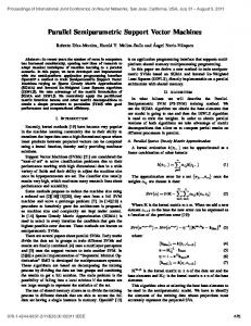
The distributed support vector machines (DPSVM) algorithm works as follows. Each site within a strongly connected network classifies subsets of training data locally via SVM and passes the calculated SVs to its descendant sites and receives SVs from its ancestor sites and recalculates the SVs and passes them to its descendant sites and so on. The algorithm of DPSVM consists of the following steps. Initialization: We initialize the algorithm with iteration t = 0 and local support vector set in site l at iteration t, V t,l = ∅, ∀l, t = 0. The training set at iteration t in site l is denoted 0,l by S t,l . The S 0,l is initialized arbitrarily such that ∪L = l=1 S S, where S denotes the total sample space. Iteration: Each iteration consists of the following steps. 1) t := t + 1. 2) For any site l, l = 1, ..., L, once it receives SVs from its ancestor sites, we repeat the following steps. a) Merge training vectors Xladd = {xi : xi ∈ V t,m , ∀m ∈ UPSl , xi ∈ / S t−1,l }, where UPSl is the set of all immediate ancestor sites of site l, to the current training sets S t,l of the current site l. b) Solve the problem (3). Record the optimal objective value ht,l and the solution αt,l . c) Find the set V t,l = {xi : αit,l > 0} and pass them to all immediate descendant sites. t,l 3) If h = ht−1,l for all l, stop; otherwise, go to step 2. Every site starts to work once it receives SVs from its ancestor sites. In step 2(b), we start solving the newly formed problem from the best solution currently available and update this solution locally. We use SVMlight [15] as our local solver. The numerical results show that the computing speed can be dramatically increased by applying the available best solution αt−1 as the initial starting point in Step 1(b). We are going to discuss this issue later in the paper. To demonstrate the convergence, we randomly generate 200 independent two-dimensional data sampled from two independent Gaussian distributions. We randomly distributed all the data to 5 sites. We assume the 5 site forms a ring network. The SVM problem is solved locally, and pass the support vectors to their descendant sites. The DPSVM converges in 4 iterations and the local results are shown in the Fig. 1. One may observe
the decreasing of the local margins and they converge to the global optimal classifier. We prove the global convergence in Section III.
maximize subject to
−(1/2)αT Qα + 1T α 0 ≤ α ≤ γ1.
(5)
where Q is the Gram matrix for all training samples. Then, t,l
Then the proof follows immediately by the fact that the solutions α ˜ t,l ∀t, l are always a feasible solution to the global problem (5) with objective value ht,l . ¶ Lemma 1 shows that each solution of the subproblem serves as a lower bound for the global SVM problem. Lemma 2: Nondecreasing: The objective value for any site, say site l, at iteration t is always greater than or equal to the maximum of the objective of the same site in the last iteration and the maximal objective values of its immediate ancestor sites, site m, ∀m ∈ UPSl , from which site l receives SVs in the current iteration. That is, ht,l ≥ max{ht−1,l , maxm∈UPSl {ht,m }} Proof. Assume t > 1 without losing generality. Let us first assume site l receives SVs only from one of its ancestor site, say site m. The solutions corresponding to the objectives ht,l , ht−1,l and ht,m are αt,l , αt−1,l and αt,m . Denote the nonzero part of αt,m by α1 . The corresponding Gram matrix is denoted by Q1 . Therefore, ht,m = −α1T Q1 α1 + 1T α1 . Define α2 = αt−1,l and the corresponding Gram matrix to be Q2 . We have ht−1,l = −α2T Q2 α2 + 1T α2 . Since some SVs corresponding to α1 may be the same as some of those corresponding to α2 , we reorder and rewrite α1 and α2 as follows: α1 = [α1a ; α1b ], α2 = [α2b ; α2c ]. So, the newly formed problem Gram matrix Qaa Q = Qba Qca ·
and we have Q1 =
for site l at iteration t has the Qab Qbb Qcb
Qaa Qba
Qac Qbc Qcc
Qab Qbb
¸
4
Fig. 1: Demonstration of data distribution in DPSVM iterations. Distribution of training data in 5 sites before iterations begins (the first row) and in iteration 1 to 4 (the 2nd to the 5th rows). This figure shows how all local classifiers converge to the global optimum classifier.
·
and Q2 =
Qbb Qcb
Qbc Qcc
¸
where Qaa , Qbb and Qcc are the Gram matrixes corresponding to α1a , α1b (or α2b ) and α2c . So The newly formed problem can be written as maximize −(1/2)αT Qα + 1T α subject to 0 ≤ α ≤ γ1. Note that [α1 ; 0; 0; . . . ; 0] and [0; 0; . . . ; α2 ] are both feasible solution of the above maximization problem with the objective value ht−1,l and ht,m respectively. Therefore, the optimum value ht,l satisfies ht,l ≥ max{ht−1,l , ht,m }. Now we remove the assumption that site l only receives SVs from site m. Since m is selected arbitrarily from l’s ancestor sites and adding more samples cannot decrease the optimal objective value (following the same argument in Lemma 1), we have that ht,l ≥ max{ht−1,l , max {ht,m }}. m∈UPSl
¶ Lemma 2 shows that the objective value of the subproblem in our DPSVM algorithm monotonically increases in each iteration. Corollary 1: The stopping criterion, ht,l = ht−1,l for all l and t > T , can be satisfied in finite number of iterations. Proof. By Lemma 2, adding SVs from the adjacent site with higher objective value results in increase of the objective value of the newly formed problem. Lemma 1 shows that
every optimal objective value for each site at each iteration is bounded by h? . Since the data points are limited and no duplicated data are allowed, ht,l = ht−1,l for all l and t > T can be satisfied in finite number of steps. ¶ Before proving our theorem, we have to prove a key proposition first. Proposition 1: If any Gram matrix formed by any training sample data sets are positive definite, and ht,l = ht−1,l = ht,l−1 = ht,l−2 = . . . = ht,l−ml where l − 1, . . . , l − ml are the ancestor sites from which site l receives SVs at the current iteration, then the support vectors sets V t−1,l , V t,m , ∀m ∈ UPSl and V t,l are equal and the solution corresponding to the SVs from either of the above site is the optimal solution for the SVM training problem for the union of the training vectors of site l and its immediate ancestor m, ∀m ∈ UPSl at iteration t. Proof. Note that at time t + 1, for site l, it is the same to update its data set by simultaneously adding SVs from site m, ∀m ∈ UPSl as to update the data set by sequentially adding SVs from those ancestor sites. That is to say, we only need to show the result in the case that site l only receives SVs from one such site, say site l − 1. Recall the notation used in the proof of Lemma: ht,l−1 = −α1T Q1 α1 + 1T α1 , ht−1,l = −α2T Q2 α2 + 1T α2 , ht,l = −αT Qα + 1T α. α1 = [α1a ; α1b ], α2 = [α2b ; α2c ]. α = [αa ; αb ; αc ]., where α1 is the nonzero part of αt,l−1 , α2 = αt−1,l and α = αt,l . The newly formed l at iteration t problem for site Qaa Qab Qac has the Gram matrix Q = Qba Qbb Qbc and we have Qca Qcb Qcc
5
·
¸ · ¸ Qaa Qab Qbb Qbc and Q2 = . Note that Qba Qbb Qcb Qcc [α1 ; 0; . . . ; 0] and [0; . . . ; 0; α2 ] are both feasible for the global optimal problem (5) and the optimal solution of this problem is α. Since, ht−1,l = ht,l−1 = ht,l , by uniqueness of optimal solution for strictly convex problem, we have αa = α1a = 0, αb = α1b = α2b and αc = α2c = 0. Since αa is nonzero, we have {α1a } = ∅.
Q1 =
This already shows that the support vectors sets V t−1,l , V t,l−1 and V t,l are identical. Then we prove that [0; ...; 0; α] is the optimal solution for the SVM problem with union of the training vector from site l and m. The Karush-Kuhn-Tucker (KKT) conditions for the problem (5) can be stated as follows: Qi α ≥ 1 Qi α ≤ 1 Qi α = 1
if αi = 0 if αi = γ if 0 < αi < γ,
where Qi is the i-th row of the Q corresponding to αi . Since [0; 0; ...; 0; α1 ], α2 and α satisfy the KKT condition of the problem P t,m , P t−1,l and P t,l where P t,l denotes the SVM problem at iteration t for site l. By simple algebra, [0; ...; 0; αb ; 0; ...; 0] satisfies the KKT condition of the SVM problem with union training vectors. Therefore, the [0; ...; 0; αb ; 0; ...; 0] is the optimal solution for the SVM problem with union of the training vector from site l and m. By sequentially adding SVs from m, ∀m ∈ UPSl , we may repeat the above argument so that our proposition is true.¶ Theorem 1: Distributed SVM over a strongly connected network converges to the global optimal classifier in finite steps. Proof. The Corollary 1 shows that the DPSVM converges in finite steps. Proposition 1 shows that when the DPSVM converges, the support vectors of each sites that are immediately adjacent are identical. Therefore, if site i can be assessed by site j, they have identical support vectors upon convergence. Since the network is strongly connected, all sites can be accessed by all other sites. Therefore, the support vectors of all sites over the network are identical. Let V ? denotes the converged support vector set. The solution defined by ½ t,l α , if xi ∈ V ? ? αi = 0, otherwise is always a feasible solution for the global SVM problem (5). By Proposition 1, V ? is also the support vector set for the union of the training samples from one site and its ancestor sites and the corresponding solution is optimal for the SVM with the union of the training samples from the those sites. As each site is accessible by all other sites by strongly connected networks, V ? is the support vector set for the union of the training samples from all sites. Therefore, the solution α? is global optimum. ¶ IV. A LGORITHM I MPLEMENTATION The proposed algorithm has an array of implementation options, including training parameter selection, network topology configuration, sequential/parallel and online/off-line implementation. Those implementation options have dramatic
impact on classification accuracy and performance in terms of training time and communication overhead. A. Global Parameter Estimation One may note that the algorithm requires that all sites use an identical training parameter γ, which balances training error and margin, such that the final converged solution is guaranteed to be the global optimum. In a centralized method, such parameters are usually tuned empirically through crossvalidations. In distributed data mining, such tuning may not be feasible given partially available training data. We, in this paper, propose an intuitive method to generate a parameter γ that has good performance to the global optimization problem by using locally available partial training data and statistics of the global training data. The training parameter γ may be estimated as follows. γ = γl
N σl2 Nl σ 2
(6)
where γl is a good parameter selected based on data in site l, and σl and σ are defined as follows. 1 X σl2 = K(xi , xi ) − 2K(xi , ol ) + K(ol , ol ) Nl i∈l
and σ2 =
1 X K(xi , xi ) − 2K(xi , ol ) + K(o, o) N ∀i
where o is the center of all training vectors and ol is the center of the training vectors at site l. Equation (6) can be justified qualitatively as follows. By formula (2), if γ is larger, the empirical error is weighted higher in the objective. That is equivalent to say, the corresponding prior is weaker for a larger γ. Some researchers choose N/σ 2 to be a default value of γ [16]. Therefore, after determining a local parameter γl at site l by cross-validation or other methods, one may expect (6) to be a good parameter for the overall problem. Our experiment results confirm such expectation. In the MNIST digit image classification discussed in the Section V, we classify digit 0 from digit 2. Suppose the 11881 training vectors are distributed into 15 sites. One may estimate parameter γ from the global optimization problem with a local optimal parameter γi at site i by (6). We use 1000 vectors as a validation set for parameter tuning and another 1000 vectors as test set. Both are sampled from MNIST test set. We first search for an local optimal γ1 at site 1 where there are 807 training vectors. Table I gives the test error over the validation set using different setting of γ. Therefore, the optimal local parameter γ1 = 2−7 . Given the global statistics σ 2 = 109.49 and the local statistics σ 2 = 110.36, we could estimate a γˆ as γˆ = γl
11881 × 110.36 N σl2 = 2−7 = 0.117. Nl σ 2 807 × 109.49
To justify the estimated parameter γˆ , we enumerate several possible value of global parameter γ, train a model based on all training vectors and obtain the test error, summarized in Table II. One may observe the best γ ? = 2−3 = 0.125. Using
6
γ1 Validation Error
2−9 0.9851
TABLE I: Validation Error at −1 Site 1 −7 −5 −3 2 0.9876
2 0.9846
2 0.9811
2 0.9811
23 0.9811
2 0.9811
TABLE II: Test Error for the Global Training Problem
2−9 0.9911
γ Test Error
1
2
3
4
5
6
2−7 0.9911
7
2−5 0.9911
8
2−3 0.9920
2−1 0.9906
2.5
1
0.994
25 0.9841
2
3
4
5
6
7
8
10
11
12
13
14
15
2
Objective Value
Test Accuracy
0.992
23 0.9886
2 0.9886
25 0.9811
0.99 1.5 0.988
0.986
1
0.984
9
Fig. 3: Diagram: a ring network.
0.5 1
0.982
2
4
0.98
1
2
3
4
5
6
7
x 10 0
3
15
8
Iteration 14 4
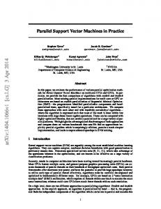
Fig. 2: Test Accuracy and Objective Value in Iterations 13
this error In this specific application, γˆ is a good estimation of the true γ ? . With the estimated γ ? , we plot the test accuracy and objective values of site 1 in each iteration of our DPSVM algorithm in Figure 2. The network we choose has 7 sites and a random sparse topology. One may observe that the objective value (of the primal problem) is monotonously increasing while the test accuracy is improving, which may not be monotonic. The power of DPSVM is to get global optimal classifier in a local site without transmitting all data into one site. B. Network Configuration Network configuration has a dramatic impact on performance of our DPSVM algorithm. Size and topology of a network determine the number of sites that may work concurrently and the frequency a site receives new training data from other sites. The size of of network is restricted by the number of servers available and number of data center distributed. The larger a network is, the more server that may work parallel, however, the more communication overhead caused as well. One may note that, upon convergence, each site must at least contain the whole set of support vectors, therefore, it is no longer very meaningful to have more than N/NSV sites while NSV denotes the number of support vectors for the global problems. Actually, Lu and Roychowdhury in 2006 showed that the number of training vector must be bounded below in order that a randomized distributed algorithm has a provably fast convergence rate [14]. Our experiments show
5
12
6
11
7
8
10 9
Fig. 4: Diagram: a fully connected network.
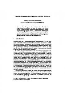
that the training speed is in general faster in a larger size of a network given the network size is limited. Network topology configuration is a key issue in implementing the distributed algorithms. Let us first consider two extreme cases: a ring network (see Figure 3 as an example) and a fully connected network (see Figure 4 as an example). A ring network is the sparsest strongly connected network while the fully connected network is the densest one. The denser a network is, the more frequently the information exchange occurs. Graf et al. in 2004 proposed a special network, namely cascade SVM, and demonstrated that the training speed in such network outperform other methods [13]. The cascade SVM is a special case of strongly connected network. Figure 5 gives a typical example. We may define a connectivity matrix C such that ½ C(k, l) =
1, 0,
if node k has an edge pointing to node l otherwise.
Without losing generality, the connectivity matrix for a ring
(7)
7
9
10
11
4
12
13
5
14
6
2
1
15
network density
8
7
3
1
0.8
0.6
0.4
0.2
Fig. 5: Diagram: a cascade network.
0 1
round−robin network fully connected network cascade network
2
0
10
20
30
40
50
60
70
size of network 3
15
Fig. 7: Network density vs network size 14 4
13
5
12
6
11
7
8
10 9
Fig. 6: Diagram: a random strongly connected network.
The lower and upper bound of the density are achieved by the ring network and fully connected network respectively. That is, 1 drr = (13) L−1 and df = 1 (14) One may calculate the density of the cascade network as follows 2p + 2p−1 − 2 dc = p , ∀p ≥ 2. (15) (2 − 1)(2p − 2)
We plot the network density against network size for the above three networks in Figure 7. A random strongly connected network (RSCN) may have a (8) topology shown in Figure 6. The network density of a RSCN may be anywhere between the solid line of ring network and A fully connected network has the corresponding connectivity dash line of the fully connected network in Fig. 7. Specifically, matrix a RSCN in Fig. 6 has its connectivity matrix Cra = ½ 0, if k = l 0 0 0 0 1 0 0 0 1 1 0 1 1 0 0 Cf (k, l) = (9) 1, otherwise 0 0 0 1 0 0 0 1 1 0 1 0 1 0 1 A typical cascade network in Figure 5 has the corresponding 0 0 0 0 1 1 1 0 1 0 1 1 1 0 0 0 0 1 0 0 1 0 0 1 0 0 0 0 1 1 connectivity matrix 0 0 0 1 0 0 1 0 0 1 0 1 0 0 0 C 0 0 0 1 0 0 0 0 1 0 0 1 1 0 0 c (k, l) = p p+1 p+1 1, if l = 2 , 2 ≤k≤2 +1 1 0 0 1 1 0 0 0 1 1 1 0 1 0 1 p q 1, if l = 2 + 2 , 0 1 1 1 1 0 1 0 1 0 0 0 0 0 0 (16) p+1 q+1 p+1 q+1 2 +2 ≤k≤2 +2 + 1, (10) 1 0 0 0 0 1 0 0 0 0 0 1 1 0 0 ∀q < p 0 1 1 0 0 0 1 0 0 0 0 0 0 0 0 p p+1 1 if k = 1, 2 ≤ l ≤ 2 − 1, p = log2 (N + 1) 0 1 0 1 0 0 0 1 0 0 0 1 1 1 0 0, otherwise 0 0 1 0 1 0 1 0 1 1 0 0 0 0 0 0 0 1 0 0 1 0 0 0 1 1 0 0 0 0 we define a density of a directed network, d as follows 0 0 0 1 0 1 1 0 0 1 0 0 0 0 0 E 1 1 1 0 0 1 0 0 1 0 0 0 0 1 0 d= (11) L(L − 1) This RSCN has 77 directed edges and 15 nodes. Its network where E is the number of directed edges and L is the number density 77 of nodes in the network. Since c(k, k) = 0, ∀k always holds dra = = 0.37. in our network configurations, we have 210 That said, it is denser than the cascade network of the 1 ≤ d ≤ 1. (12) same size. In our experiments, we try a variety of network L−1 network has the following form ½ 1, if l = k + 1, k < L or k = L, l = 1 Crr (k, l) = 0, otherwise
8
topologies. The results show that the cascade networks are not the ”golden” density positions. A random network of the same size, such as the one in Fig. 6, may achieve better performance in terms of training speed. C. Synchronization Other than network topology, timing of local computing also plays an important role on the effect of data accumulation and therefore the training speed. In this paper, we discuss two timing strategies: synchronous and asynchronous implementations. One strategy is to process local data upon receiving support vectors from one site’s all immediate ancestor sites. For example, in network defined in Figure 6, in second and later iteration, site 1 will start processing once having received data from site 7, 9 and 15, given it is currently idle. One may also observe this from the first column of (16). We call this strategy synchronous implementation as each server needs to wait for all of its immediately ancestor sites to finish processing. Another strategy is called asynchronous implementation. In this strategy, each site processes its data upon receiving new data from any of its immediate ancestor sites. For example, in network defined in Figure 6, in second and later iteration, site 1 will start processing once having received data from either site 7, 9 or 15, given it is currently idle. Asynchronous implementation guarantee that all server are utilized as much as possible. The advantage and disadvantage of both implementation strategies are empirically compared in Section V. D. Online Implementation Since the DPSVM constructs a local problem by adding critical data, local SVM training problems in subsequent iterations are essentially problem adjustments which append variables and constraints based on the problem of the last iteration. Online algorithm is a popular solution for incremental learning problems. In this paper, we compare a simple online algorithm with an off-line algorithm. In the simple online implementation, at each iteration, every site always uses current dual solution (α values) as its initial α values. The newly added training data will also bring a vector of non-zero α’s. We use a slightly modified SVMlight [15] as our local SVM solver, which may take an arbitrary α vector as input. To avoid possible infinite loops due to numerical inaccuracies in the core QP-solver, a somewhat random working set is selected in the first iteration and we do it for every 100 iterations. Our experiments in Section V show that this simple on-line implementation greatly improves the distributed training speed over the off-line implementation. V. P ERFORMANCE S TUDIES We test our algorithm over a real-word data set: MNIST database of handwritten digits [17]. The digits have been sizenormalized and centered in a fixed-size image. This database is a standard database online for researchers to compare their
training method because MNIST data is clean and doesn’t needs any preprocessing. All digit images are centered in a 28x28 image. We vectorize each image to a 784 dimension vector. The problem is to classify digit 0 from digit 2, which involves 11811 training vectors. A linear kernel is applied in all experiments to simply the parameter tuning process. We first introduce our terminology used in this section. N : total number of training samples; L: total number of distributed sites; E: total number of directed edges in the network; d: density of network; Nsv : total number of global support vectors; T : total number of DPSVM iterations; δ: total number of transmitted data per time; ∆: total number of transmitted vectors; Nl,t : number of training samples in site l at iteration t; max{N.,. }: maximum number of training samples among all sites among all iterations; e: elapsed CPU seconds of running DPSVM; ς: the standard deviation of initial training data distribution. Throughout this section, the machines we use to solve local SVM problem are Pentium 4 3.2GHz with 1GB RAM. A. Effect of Initial Data Distribution In real world applications, data may be distributed arbitrarily around the world. In certain applications, the distributed data may not be balanced or unbiased. For example, search engine companies usually need to classify Web pages for different markets, where the document data are usually stored locally due to both legal and technical constraints. Those data are highly unbalanced and biased. For example, China market may contain much less business pages than US market. In other applications, the data may be evenly distributed, intensionally or naturally. For example, Unites States Citizen and Immigration Services (USCIS) often distributes cases to their geographically distributed service centers to balance workloads. To analyze the effect of initial data distribution, we randomly distribute the 11811 training data to a fully connected network with 15 sites. We do this several times with different settings of standard deviation of data distribution. When the data are distributed evenly, the standard deviation of the initial data distribution, ς is approximately 0. When ς is larger, the distributed more unbalanced. We run our DPSVM for ς = 0, 305.7, 610.7 respectively. We also test a special portional distribution where all data are initially distributed into 8 sites only and the rest 7 sites are left empty. This particular distribution has ς = 766.9. In a four-layer binary cascade network, the data are initially distributed into the first layer under this distribution. The total communication cost ∆ and elapsed training time e against the initial data distribution are summarized in Table III. The results show that evenly distributed data may result in a fast convergence (less iteration and shorter cpu time) while the special portional distribution (8 sites of data and 7 empty sites) obviously achieves less communication overhead.
9
TABLE III: Performance over the initial data distribution ς
T
0 305.7 610.7 766.9?
8 8 8 6
0 305.7 610.7 766.9?
16 17 18 18
δ¯ ∆ maxl,t {Nlt } Random Dense Network 126 15191 1836 115 13897 2086 130 15363 2247 102 12247 2097 Binary Cascade Network 37 8842 1008 35 8977 1569 30 8120 1653 26 6906 1731
e
9.00 8.93 12.32 16.92 15.51 15.63 17.20 16.43
? : Training data are evenly distributed in 8 sites. The other 7 sites are empty before receiving any support vector from other sites.
TABLE IV: Tested Network Configurations L 3 3 3 7 7 7 7 7 15 15 15 15 15
Topology ring binary-cascade fully connected ring binary-cascade random sparse random dense fully connected ring binary-cascade random sparse random dense fully connected
E 3 4 6 7 10 14 33 42 15 22 54 159 210
d 0.50 0.67 1.00 0.17 0.24 0.33 0.79 1.00 0.07 0.10 0.26 0.76 1.00
observed from the number of iterations in Fig. 8 (b). One may also observe that a random dense network may outperform binary cascade SVM in terms of training time when the network size is not too small. In a small network, a fullyconnected network has its advantage over other topologies. Fig 8 (c) shows the fact that the communication cost per site is not flat when size of the network is increasing. Therefore, the total communication overhead increase faster than the network grows. The reason is due to synchronization. That is, each site has to wait and accumulate data from all of its ancestor sites in each iteration. This issue will be further discussed in Section V-D. C. Effect of Online Implementation We implement a simple online algorithm described in Section IV-D. To show its effect, we plot the computing time in each iteration at site 1 in Fig. 9. One may observe that in off-line implementation, the computing speed heavily depends on the absolute number of SVs. On the other side, the online computing time is more sensitive to the change of the number of SVs. The initial sharp increase of CPU seconds is due to the sharp increase of number of local SVs. The later decreasing of CPU seconds is due to the advantage of online implementation. D. Effect of Server Synchronization
B. Scalability on Network Topologies We test our algorithm over an array of network configurations. Five network topologies are tested including ring networks, binary cascade networks, fully connected networks, random sparse networks and random dense networks. For the two types of random networks, we impose a constraint over the network density such that d ≤ 0.33 for random sparse networks and d ≥ 0.75 for random dense networks. Networks of 3, 7 and 15 sites are tested for ring, binary cascade and fully connected networks. Networks of 7 and 15 sites were tested for the two types of random generated networks. The number of sites, number of edges and the corresponding network densities of all tested networks are summarized in Table IV. In this section, we apply online and synchronized implementation for each tested networks. The off-line and asynchronous implementation will be discussed later. We record the total training time in terms of elapsed CPU-seconds, the number of iterations, and the number of transmitted training vectors per site. The results are plotted in Fig. 8. The results show that our algorithm scales very well for all network topologies except for the ring network, given the size of the network is limited. In ring networks, however, one site’s information reach all other sites only after as least L − 1 iterations. The communication is therefore not efficient and the convergence becomes slow. The convergence over a variety of network topologies can be
Recall that each site may start processing its local training vectors every time when it receives a batch of training data from one of its ancestor sites. We call it asynchronous implementation. Another implementation is to let each site wait until it receives new data from all of its ancestor sites. We call it synchronous implementation. We implement the two strategies in a variety of networks. We compare their total training time and communication overhead for each of networks in Fig. 10 and Fig. 11 respectively. One may observe that, except for the cascade network, the synchronous implementation always dominates asynchronous one in terms of total training time. The reason that the difference of a synchronous and asynchronous is small in cascade networks is probably due to the fact that the topology of the cascade network already ensures certain synchronization. A more interesting result is in Fig. 11, where one may observe that the communication cost increases almost linearly with network size in asynchronous implementations and slower than synchronous implementations. The scenario can be explained as follows. In asynchronous implementation, since there are always sites that processes slower than other sites, the computing and communications are more frequent among those faster sites. The network that is effectively working is actually smaller since those slower sites contributes relatively less. As we know that a small network usually has longer processing time and less communication cost, the asynchronous implementation is similar as using a smaller network. E. Performance Comparison Between SVM and DPSVM When merging all training data is infeasible due to physical or political reasons, one may apply the DPSVM that is able to
10
Iteration 0
1
18
Round Robin Binary Cascade Random Sparse Random Dense Fully Connected
CPU Seconds
120
4
5
6
7
8
9
10 350
300
16
CPU Seconds
140
3
Offline Impl. Online Impl.
(a) Elapsed Training Time 160
2
100
80
60
250
14
12 200 10 150 8
6
100
4
40
50 2
Number of Support Vectors
20
20
0 0
2
4
6
8
10
12
14
1
2
3
4
5
6
7
8
9
0
16
Size of Network
Fig. 9: Effect of the online implementation.
(b) Num of Iterations 50
Round Robin Binary Cascade Random Sparse Random Dense Fully Connected
45
Total Number of Iterations
The number of support vectors and the computing time of site 1 per iteration DPSVM, implemented over a random sparse network with 15 sites. The solid line is the computing time per iteration for on-line implementation. The dashed line represents the computing time per iteration for off-line implementation. The bars represent the number of support vectors per iterations. The figures demonstrates that the computing time of off-line implementation also depends on the number of support vectors, while the online implementation does not.
40
35
30
25
20
15
10
5
0
2
4
6
8
10
12
14
16
Total Number of Transmitted Vectors Per Site
Size of Network (c) Communication Per Site 1200
Round Robin Binary Cascade Random Sparse Random Dense Fully Connected
1100
1000
Binary Cascade Sync. Async
150
900
Random Sparse Sync. Async
150
800
100
100
50
50
700
600
500
0
0
5
10
15
0
0
5
10
15
400
300
Random Dense 2
4
6
8
10
12
14
Fully Connected
16
Size of Network
Sync. Async
150
Fig. 8: Performance over Network Configurations.
Five network topologies are compared. Top. The elapsed CPU seconds of training time over size of networks. Middle. The number of iterations over size of networks. Bottom. The total number of transmitted training vectors per site upon convergence over size of networks.
150
100
100
50
50
0
0
5
10
15
0
Sync. Async
0
5
10
Fig. 10: Training Time of Async. and Sync. Impl.
15
11
4
2
x 10
Binary Cascade
4
2
x 10
Sync. Async
Sync. Async
1.5
1.5
1
1
0.5
0.5
0
0
5
4
2
x 10
10
15
0
Random Dense
0
x 10
Sync. Async
1
1
0.5
0.5
5
10
15
Fully Connected Sync. Async
1.5
0
5
4
2
1.5
0
Random Sparse
10
15
0
0
5
10
15
Fig. 11: Communication Overhead of Async. and Sync. Impl.
TABLE V: Tested Accuracy of DPSVM and Normal SVMs L 1 3 7 15
DPSVM 0.9920 0.9920 0.9920 0.9920
Min (SVM) 0.9920 0.9881 0.9871 0.9806
Max (SVM) 0.9920 0.9916 0.9911 0.9891
• The DPSVM algorithm is able to work on multiple arbitrarily partitioned working sets and achieve close to linear scalability if the size of network is not too large. • Data accumulation during SVs exchange is limited if the overall SVs are limited. Communication cost is proportional to the number of SVs. Asynchronous implementation over a sparse network achieves the minimum data accumulation. • The DPSVM algorithm is robust in terms of computing time and communication overhead to the initial distribution of the database. It is suitable for classification over arbitrary distributed databases as long as a network is denser than the ring network. • In general, denser networks achieve less computing time while sparser networks achieve less data accumulation. • On-line implementation is much faster. A fast on-line solver is critical for our DPSVM algorithm. This is also one of our future research directions.
Mean (SVM) 0.9920 0.9903 0.9878 0.9854
reach a global optimal solution or the normal support vector machine that works on local data only. We demonstrate that our DPSVM has the real advantage in terms of test accuracy over normal SVMs that are trained based on local training data. We compare the DPSVM and SVM when MNIST data are randomly distributed into 3, 7 and 15 sites assuming that each site has the same number of training vectors. The training parameter is estimated following the approach introduced in Section IV-A. We compare the test accuracy of the DPSVM to the minimum, maximum and average value of the test accuracy of normal SVM among all sites. The results are summarized in Table V. The table shows expected phenomena: the less training are used, the worse the test accuracy is achieved. This is one of the motivations of the DPSVM: to reach global optimum and better test performance without aggregating all the data. VI. C ONCLUSIONS AND F UTURE R ESEARCH The proposed distributed parallel support vector machine (DPSVM) training algorithm exploits a simple idea of partitioning training data and exchanging support vectors over a strongly connected network. The algorithm has been proved to converge to the global optimal classifier in finite steps. Experiments over a real-world database show that this algorithm is scalable and robust. The properties of this algorithm can be summarized as follows.
R EFERENCES [1] Y. Zhu and X. R. Li, “Unified fusion rules for multisensor multihypothesis network decision systems,” IEEE Transactions on Neural Networks, vol. 33, pp. 502–513, July 2003. [2] V. Vapnik, The Nature of Statistical Learning Theory. New York: Springer Verlag, 1995. [3] C. Cortes and V. Vapnik, “Support-vector networks,” Machine Learning, vol. 20, pp. 273–297, 1995. [4] H. Drucker, D. Wu, and V. N. Vapnik, “Support vector machines for spam categorization,” IEEE Transactions on Neural Networks, vol. 10, pp. 1048–1054, September 1999. [5] L. Cao and F. Tay, “Support vector machine with adaptive parameters in financial time series forecasting,” IEEE Transactions on Neural Networks, vol. 14, pp. 1506–1518, November 2003. [6] S. Li, J. T. Kwok, I. W. Tsang, and Y. Wang, “Fusing images with different focuses using support vector machines,” IEEE Transactions on Neural Networks, vol. 15, pp. 1555–1561, November 2004. [7] L. M. Adams and H. F. Jordan, “Is SOR color-blind?” SIAM Journal on Scientific and Statistical Computing, 1986. [8] U. Block, A. Frommer, and G. Mayer, “Block coloring schemes for the SOR method on local memory parallel computers,” parallel Computing, 1990. [9] G. Zanghirati and L. Zanni, “A parallel solver for large quadratic programs in training support vector machines,” Parallel Computing, vol. 29, pp. 535–551, November 2003. [10] N. Syed, H. Liu, and K. Sung, “Incremental learning with support vector machines,” in Proceedings of the Fifth ACM SIGKDD International Conference on Knowledge Discovery and Data Mining (KDD), San Diego, California, 1999. [11] C. Caragea, D. Caragea, and V. Honavar, “Learning support vector machine classifiers from distributed data sources,” in Proceedings of the Twentieth National Conference on Artificial Intelligence (AAAI), Student Abstract and Poster Program, Pittsburgh, Pennsylvania, 2005. [12] A. Navia-Vazquez, D. Gutierrez-Gonzalez, E. Parrado-Hernandez, and J. Navarro-Abellan, “Distributed support vector machines,” IEEE Transaction on Neurual Networks, vol. 17, pp. 1091–1097, 2006. [13] H. P. Graf, E. Cosatto, L. Bottou, I. Durdanovic, and V. Vapnik, “Parallel support vector machines: The cascade SVM,” in Proceedings of the Eighteenth Annual Conference on Neural Information Processing Systems (NIPS), Vancouver, Cannada, 2004. [14] Y. Lu and V. Roychowdhury, “Parallel randomized support vector machine,” The 10th Pacific-Asia Conference on Knowledge Discovery and Data Mining (PAKDD 2006), pp. 205–214, 2006. [15] T. Joachims, “Making large-scale SVM learning practical,” Advances in Kernel Methods - Support Vector Learning, pp. 169–184, 1998. [16] ——, “Svm-light support vector machine,” 1998. [Online]. Available: http://svmlight.joachims.org/ [17] Y. LeCun, L. Bottou, Y. Bengio, and P. Haffner, “Gradient-based learning applied to document recoginition,” Proceedings of the IEEE, vol. 86, no. 11, pp. 2278–2324, November 1998.