Revised submission to the 11th International Machine Learning Conference ML-94
Consideration of Risk in Reinforcement Learning
Matthias Heger Zentrum für Kognitionswissenschaften, Universität Bremen Postfach 330 440 D-28334 Bremen, Germany email:
[email protected] Tel.: +49 (0) 421 218 4659 Fax: +49 (0) 421 218 3054 Abstract Most Reinforcement Learning (RL) work supposes policies for sequential decision tasks to be optimal that minimize the expected total discounted cost (e. g. QLearning [Wat 89], AHC [Bar Sut And 83]). On the other hand, it is well known that it is not always reliable and can be treacherous to use the expected value as a decision criterion [Tha 87]. A lot of alternative decision criteria have been suggested in decision theory to get a more sophisticated considaration of risk but most RL researchers have not concerned themselves with this subject until now. The purpose of this paper is to draw the reader’s attention to the problems of the expected value criterion in Markov Decision Processes and to give Dynamic Programming algorithms for an alternative criterion, namely the Minimax criterion. A counterpart to Watkins’ Q-Learning related to the Minimax criterion is presented. The new algorithm, called Q$ − Learning , finds policies that minimize the worst-case total discounted costs. Most mathematical details aren’t presented here but can be found in [Heg 94].
Keywords: reinforcement learning, computational learning theory
1. Introduction In the paradigm of Reinforcement Learning (RL), an agent interacts with an environment (world) and, simultaneously, receives reinforcement signals which are punishments or costs caused by single decisions and/or state-transitions1. The learning task is to find a favorable policy, i.e., a rule that tells the agent what action to choose in what situation. The most frequently used model of the interaction between the agent and the world is a special kind of stochastic process, namely the Markov decision process (MDP) that will be introduced in the following. Three sets are elementary in MDP: The set S of the environment’s states from the agent’s point of view, the set A of the agent’s actions and the set C of the reinforcement signals which, in the following, will be also called immediate costs. In this paper we confine ourself to finite sets S and A represented by subsets of N. The elements of C ⊂ R are assumed to be countable, bounded and nonnegative. In general, the agent must not or is not able to select an arbitrary action in every state. The nonempty set A i ⊆ A is the set of admissible actions in state i.
af
The agent’s interaction with the world is divided into a sequence of so-called stages or episodes. In the following, a paradigm of an episode is given: First, the agent observes a starting state i ∈ S and has to choose an action a ∈ A(i). Then, a state transition occurs from state i into a successor state j ∈ S . Finally, the agent receives a scalar reinforcement signal r. The immediate cost r represents the effort of the state transition from i to j under action a. We assume time to be discrete. It is essential in MDP that at any time t, the probability to get a certain successor state j depends on the starting state i and the action a of episode t but not additionally on the time and history of episodes. Ps(i, a, j) represents the probability that the successor state of an episode is j if starting state i and action a is given. Similarly, at any time t, the probability to get a certain immediate cost depends on the starting state, the action and the successor state of episode t but nor additionally on the time nor on past episodes. Pc(i, a, j, r) stands for the probability that the immediate cost of an episode is r if the starting state i, the action a and the successor state j is known.
1In
literature, reinforcement signals often also represent rewards, but it is well known that the reward representation can easily be transformed into the cost representation and vice versa.
2
In MDP, the starting state of episode t equals the successor state of episode t-1 for all t > 0. The starting state of episode zero may be given by a probability
af
distribution. P0 i denotes the probabilty that i is the starting state of the episode with the time index t = 0. For technical reasons we suppose P0 i > 0 for all i ∈ S.
af
The agent’s behavior is specified by a policy which is a rule that yields an action in any given situation. In a comprehensive model of policies, the agent may consider at any time the current state, the time and the past states and actions in order to select an action. Additionally, the selection of the action may be done probabilistically. Action selection by the so called stationary policies only require the agent to consider the current state. These policies identifies with merely mappings from states to actions. States and immediate costs are random variables in MDP because of the probabilistic nature of the immediate costs and state transitions. These random variables essentially depends on the policy applied by the agent. Therefore, the following notation is used: Itπ denotes the starting state and the notation for the immediate costs is Ctπ , where it is assumed that the agent uses policy π and the index t represents the time index of the episode. 2. Problems with the Expected Value Criterion In this section we introduce the commonly used measure of performance for policies and emphasize some drawbacks. For the remainder of the text assume γ ∈ 0, 1 . We concentrate on
f
Rγπ, 0 : = 0, Rγπ, t : = where π is a policy and t ∈ N+.
t −1
∑ τ = 0 γ τ Cτπ
and Rγπ : =
∞
∑ τ = 0 γ τCτπ
Rγπ is called the (discounted) return (of π) or the total (discounted) cost. By the return all immediate costs are taken into account and because of the discount factor γ, costs are wheighted the less the more distant they lie in the future. The total discounted cost is to be found often in RL because a lot of problems as, e.g., goal tasks or time-until-success tasks and time-until-failure tasks [Sut 84] can be
3
represented by the task of finding a policy which minimizes the total cost. Rγπ, t is the t-step (discounted) return (of π) and is important because it may serve as an approximation for Rγπ . The return by itself is not an ordered measure of performance for policies and it is not trivial to derive one from the return. The problem arises from the fact that the return Rγπ is not a real number but a random variable. In deterministic domains, random variables identifies with real numbers and, undoubtedly, in such domains the agent should find a policy that minimizes the total cost. But what policy is to be preferred in probabilistic domains? The usual answer for this problem in RL is to concentrate on the expected value of the return as it is also done in Q-Learning and the AHC architecture [Sut 91]. More precisely, most RL researchers measure the performance of a policy π by Ee Rγπ I0π = i j , i.e., the expected value of the return relating to a given starting state i of episode 0. π is usually called optimal if it minimizes Ee Rγπ I0π = i j for each i ∈ S . In operations research and decision theory (e.g. [Tah 87]), however, it is well known that it is not always reliable and can be treacherous to use the expected value as a decision criterion. We give three simple examples from decision theory [Bra 76] that show different problems of the criterion of expectation. The first problem is revealed by the celebrated St. Petersburg Paradox. A man offers you the privilege to play the following game for a stake of k dollars: A fair coin is to be tossed repeatedly until a head comes up. If it comes up head on the first toss, your opponent pays you two dollars. If a head first comes up on the second toss you get four dollars. And, in general, if the first head comes up on the nth toss, you receive 2n dollars. The probability that the first head comes up on the nth toss is 1/2n. The expected value of the game’s payoff X is Ea X f =
∞
1
∑n =1 2 n 2n − k
=
∞
∑ n =11n − k
4
= ∞ − k = ∞.
If you decide not to play the game, the expected payoff is of course zero. Therefore, by the expected value as a decision criterion, you have to decide to play the game for any finite stake. But no one would put up an arbitrary high stake to play a game in which recouping one's stake has "infinitesimal" small probabilities. The amount of the possible gain is appreciable enough but the probability of obtaining it is too small. The second example is a lottery in which there are 10,001 tickets, of which 10,000 are winners and only one is a loser. It costs $100 to buy a ticket; if you win you get $100.01 and if you lose you get nothing. The expected value for the payoff X of the game is E a X f =
1 10 , 000 a $100 . 01f + a $0 f − $100 = $0 . 10 , 001 10 , 001
Hence, by the criterion of expectation it is equivalent to decide to play or not to play the game. On the other hand, most people would undoubtedly decide not to play the game because the possible gain of one cent is too small to risk the loss of the stake of $100. This decision is hardly influenced by the fact that the probability for the loss is very small. Finally, consider the plight of a businessman who has $1,000 cash and no credit and who must raise an additional $100,000 immediately or lose his business. A gambler offers him the following gamble: the businessman makes a single throw with a pair of fair dice; if the dice come up 2 or 12, the gambler pays the businessman $10,000, but if any other number comes up, the businessman pays the gambler $1,000. The expected value for the payoff X of the game is −$7, 000 = −$388. 89. 18 By the criterion of expectation, the businessman has to decide not to play the game. Yet it is definitely to his advantage to take the gamble. Subjective values are not considered by the criterion of expectation. 1I H 18 K
E a X f = $10 , 000 F
17 I H 18 K
+ a −$1, 000 fF
=
We give an extension of the summary from [Bra 76]: The expected value as a criterion for action in choice behavior (a) is based upon long-run considerations where the decision process is repeated a sufficiently large number of times under same conditions. It is not
5
necessarily a valid criterion in the short run or one-shot case, especially when either the possible consequences or their probabilities have extreme values. (b) assumes the subjective values of the possible outcomes are proportional to their objective values, which is not necessarily the case, especially when the values involved are large. The decision problem, we are confronted in MDP, is the question what policy is to be used by the agent if the current state i of the world is given. In our framework, the outcome of a decision for a policy is its return. Since all immediate costs of the future are involved by the return, it needs an infinite amount of time until the outcome of the decision is present. Therefore the agent has no time to repeat the decision process, and there is by definition no possibility to satisfy the long-run condition as mentioned in (a). In practice, however, this does not imply that long-run considerations are generally out of the question because the return may be approximated by the t-step return where t ∈N is assumed to be sufficiently large. The more important issue whether long-run considerations are adequate to measure the performance of a policy related to starting state i exists in the condition that the agent shall and will visit i sufficiently often. This condition essentially depends on the domain and the agent’s task. In the MDP of figure 1, e.g., there is no admissible sequence of actions that will eventually bring the world in state 0 more than once. In this domain, long-run considerations related to state 0 are adequate only then if one assumes events not involved in the MDP that may transfer the world in state 0 sufficiently often. In the following, the significance of (b) is to be considered, i.e., the problem of subjective values of the decision’s outcome. Assume a so-called utility function U: R → R that maps the value of the decision’s outcome, i.e. the return, into a subjective value. In general, we have F ∞
I
H τ=0
K
U e Rγπ j = U G ∑ γ τ Cτπ J ≠
∞
∑ γ τU eCτπ j .
τ=0
Therefore, the problem of maximizing the subjective value (utility) of the return is generally not equivalent with the task to maximize the discounted sum of utilities
6
of the immediate costs. Hence, the problem of subjective values is not merely to solve by an easy redefinition of the underlying cost model in the MDP. In [Koe Sim 93] this problem is discussed for planning tasks.
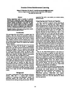
x ∈S 0 1 2
πa x f ∈ Aa x f µ a x f ∈ Aa x f
0 0 0
1 0 0
Figure 1: In this MDP, denoted by a state transition graph, there are three states (circles). A state transition from a starting state i to a successor state j is represented by a directed edge labeled by a triple. The first number a in the triple is an admissible action a for state i. The second number stands for the probability that the state transition will occur if action a is selected in the corresponding starting state i. Finally, the third number represents the immediate cost for the transition. The table denotes the only two possible stationary policies π and µ . 3. Decision Criteria There are several alternatives to the decision criterion of expectation designed in decision theory in order to have a more sophisticated consideration of risk. Two categories of decision-making situations are to be considered in nondeterministic domains: Decision under risk and decision under uncertainty. In the first category all probability distributions that specify the domain are known, whereas in the second category no probability density function can be secured. Since we concern ourself with the definition of an optimal (decision for a) policy, the definition should be based on all information that specify the domain of the MDP. Therefore, we concentrate on decision under risk. To give a very short list of some criteria of decision under risk, we use, as an example, our decision problem of what policy to be used by the agent if the current state i of the world is given. For more criteria and a discussion of the following criteria see e.g. [Tah 87].
7
As mentioned above, by the expected value criterion a policy π is to be selected that minimizes Ee Rγπ I0π = i j . The expected utility theory criterion comes from utility theory [Neu Mor 47]. A utility function U: R → R is to be assumed that maps the value of the return into a subjective value. A policy π is to be selected that maximizes EeU e Rγπ j I0π = i j . Problem (a) and (b) of the criterion of expectation can be considered by the expected utility criterion. Unfortunately, although guidelines for establishing utility functions have been developped, utility is a rather subtle concept that cannot be quantified easily [Tah 87]. By the expected value-variance criterion a policy π is to be chosen that minimizes Ee Rγπ I0π = i j − K ⋅ var e Rγπ I0π = i j where K is a prespecified constant which is sometimes referred to as risk aversion factor. Because in our framework reinforcement signals are costs, K is assumed to be negative. The α-value [Heg 94] of the return of policy π related to state i is defined as follows: m$ α : = m$ α e Rγπ I0π = i j : = sup{r ∈ R: Pe Rγπ > r I0π = i j > α} where α ∈ 0, 1 and Pe Rγπ > r I0π = i j denotes the probability that the return is greater than r if the starting state i of episode 0 is given. In [Heg 94] it is shown
f
that Pe Rγπ ≤ m$ α I0π = i j ≥ 1 − α . Therefore the agent which starts in state i and uses policy π has the security that, at least with probability 1-α, the total cost will not exceed m$ α . On the other hand, the agent has to be aware of the risk that the total cost will exceed any number less than m$ α with a probability greater than α. By the α-value criterion a policy is to be chosen that minimizes m$ α . See [Heg 94] for an extended discussion of this criterion.
8
4. Dynamic Programming (DP) for the Minimax Criterion For the remainder of the text we restrict our attention to the minimax criterion which is a special case of the α-value criterion where α = 0. We call Vγπ ai f : = m$ 0 e Rγπ I0π = i j = sup{r ∈ R: Pe Rγπ > r I0π = i j > 0} the max-value of the return of policy π related to state i. The name max-value comes of the fact that Pe Rγπ ≤ Vγπ ai f I0π = i j = 1 and Pe Rγπ > r I0π = i j > 0 for every r < Vγπ i . Hence the agent which starts in state i and uses policy π can be
af
sure that the total costs will not exceed Vγπ i . But the agent has to be aware that
af
the return will exceed any number less than Vγπ i with a positive probability. In
af
other words, Vγπ i can be seen as the worst (i.e. maximum) value of the total
af
costs that can occur if the agent uses π and starts in state i. Imagine domains where it is to be guaranteed that the return will not exceed a given threshold r if the agent starts in state i. This constraint is satisfied iff a policy π is used that satisfies Vγπ i ≤ r . Examples for such domains are those goal tasks where the agent has to reach a goal within in certain time with probability 1. The criterion of expectation is not adequate for these tasks in the framework of an MDP. This motivates the following alternative measure of performance for policies.
af
We measure the performance of a policy π by the value function Vγπ which maps any i ∈ S into Vγπ i ∈ R, and we define the optimal value function Vγ∗ i ∈ R S by
af
af
∀i ∈ S: Vγ∗ ai f : = inf Vγπ ai f . π
We call a policy π optimal (related to the minimax criterion) if its value function Vγπ equals the optimal value function Vγ∗ .
9
Before going on with the theory of the minimax criterion we give an example that reveals the utility of this criterion. In figure 1, e.g., Ee Rγπ Iγπ = 0 j = 309 + 2 γ , Ee Rγµ I γµ = 0 j = 310 + 2 γ , Vγπ 0 = 400 + 2 γ and Vγµ a0 f = 310 + 2 γ . Policy µ is optimal related to the minimax criterion and ensures that the return will not exceed 310+2γ if the agent starts in state 0 whereas the worst-case return for π is 400+2γ. Policy π is optimal related to the expected value criterion but there is only a difference of one cost unit for the expected return of µ. Therefore, policy π and µ have nearly the same performance related to the criterion of expectation. But with probability 0.75, the policy π will lead to a total cost of 400+2γ that is 90 units greater than the total cost of the minimax-optimal policy µ if the agent starts in state 0.
af
In [Heg 94], theory of DP for the minimax criterion is presented. It follows a short summary of the most essential results. Let N(i, a) be the set of states that immediately can be reached from state i by action a, i.e., more precisely, N ai, a f : =
mj
∈ S: Ps ai, a, j f > 0r .
Furthermore, let C$ ai, a, j f be the worst immediate cost that can occur in the transition from state i into state j under action a, i.e., to be precisely, C$ ai, a, j f : = supmr ∈ C: Pc ai, a, j , r f > 0r. Theorem 1: Let π ∈ AS be a stationary policy, v0 ∈R S and vk +1 ai f : =
max
j ∈ N bi , πa i fg
C$ bi, π ai f, j g + γ ⋅ vk a j f
for all i ∈ S and k ∈N. Then vk ∈R S converges to Vγπ as k → ∞. Theorem 2: Let v0 ∈R S and vk +1 ai f : =
I F C$ ai, a, j f + γ ⋅ vk a j f J G max a ∈ A a i fH j ∈ N a i , a f K
min
for all i ∈ S and k ∈N. Then vk ∈ R S converges to Vγ∗ as k → ∞.
10
Theorem 3: A stationary policy π ∈ AS is optimal if and only if it satisfies ∀i ∈ S:
F
π ai f = arg min G max
$ a i , a, j f + γ eC
a∈Aai f H j ∈N a i , a f
I
⋅ Vγ∗ a j fjJ . K
Theorem 1 yields a DP algorithm to compute the value function of a stationary policy π and by the algorithm of theorem 2 the optimal value function can be found. The algorithms use synchronous updating but we suspect that, by analogy with DP for the criterion of expectation ( e.g. [Bar Bra Sin 93], [Wil Bai 93]), convergence holds for asynchronous forms of DP as well. Theorem 3 implies that there is at least one stationary optimal policy. From theorem 2 and 3 we see that all stationary optimal policies can be computed if the sets N(i, a) and the worst immediate costs C$ ai, a, j f are known for all i, j ∈ S and a ∈ A. In contrast to DP for the criterion of expectation [Ros 70], it is not necessary to know complete probability distributions for state-transitions. 5. Q$ − Learning We present the algorithm Q$ − Learning [Heg 94] which can be regarded as the counterpart to Watkins’ Q-Learning [Wat 89] related to the minimax criterion. Consider the function Q$ γ∗ that maps all admissible state-action pairs, i.e. pairs of states and admissible actions, into real numbers and that is defined by ∀i ∈ S ∀a ∈ Aai f: Q$ γ∗ ai, a f : =
max
∗
$ a i , a , j f + γ ⋅ V a j fj . eC γ
j ∈N ai , a f
Theorem 3 implies that a stationary policy π ∈ A S is optimal if and only if it is greedy related to Q$ γ∗ , i.e., π satisfies πai f = arg min Q$ ∗ ai, a f for all i ∈ S . The aim a ∈Aa i f
of Q$ − Learning (see figure 2) is to learn Q$ γ∗ which, as we have seen, is a key to determine optimal policies. In [Heg 94] it is shown that the Q-function in Q$ − Learning converges with probability one to Q$ γ∗ as the number of iterations
11
goes to infinity if the following condition is satisfied2: The Q-function is represented by a table and every pair of starting state and action occurs infinitely often. Consider the condition that the Q-function is represented by a table, every state becomes infinitely often a starting state and the agent chooses always greedy actions related to its current Q-function. We suspect that, in most cases, under this condition the Q-function converges to an approximation of Q$ γ∗ that is sufficient to determine optimal policies. See [Heg 94] for a discussion of this issue.
1. Initialize Q(i,a) := q(i,a) for all i ∈ S and a ∈ A i where q(i,a) ≤ Q$ γ∗ i, a ; 2. i := starting state of current episode; 3. Select an action a ∈ A(i) and execute it; 4. j := successor state of current episode; 5. r := immediate cost of current episode;
af
L
a f
O
6. Qai, a f : = max MQai, a f, r + γ ⋅ min Qa j , b fP ; N
b ∈Aa j f
Q
7. Go to Step 2. Figure 2: The Q$ − Learning algorithm. If there is no apriori knowledge about Q$ γ∗
then the init-values q(i,a) can be set to zero since 0 ≤ Q$ γ∗ i, a for all states i and
a f
actions a ∈ A i
af
Experimental tests with Q$ − Learning are still to be done but we suspect pleasant and quick behavior of convergence since there are no learning rates and all Qvalues are monotone increasing related to time. Both is generally not the case in QLearning.
2Convergence
does not depend on the condition that the successor state of an episode equals the starting state of the following episode.
12
In deterministic domains Q$ − Learning identifies with Q-Learning if in the latter all Q-values are initialized as in Q$ − Learning and if the learning rates in Q-Learning are set to one. Hence, the complexity analysis of Q-Learning in determinstic domains [Koe 92] holds for Q$ − Learning . 6. Related Work The modification of Q-Learning presented in [Heg Ber 92] is a preliminary algorithm of Q$ − Learning . It is also based on the minimax criterion but no convergence is ensured in probabilistic domains and it is not memoryless. It has been applied successfully in the coordination of the six legs of a simulated walking machine. More mathematical details of the α-value criterion, the minimax criterion including DP and Q$ − Learning can be found in [Heg 94]. DP algorithms with different notation and representation of uncertainty of the MDP for the minimax criterion can be also found in [Ber Rho 71]. 7. Conclusions and Future Work This paper emphasizes the problems of the criterion of the expected return as a measure of the performance for policies. Despite the fact that a lot of work has been done in decision theory in order to get decision criteria that consider the phenomenon risk more sophisticatedly than the criterion of expectation, RL research is dominated by the expected value criterion until now. RL algorithms that are based on different decision criteria are still to be designed. Especially in domains where it is to be ensured that the total costs will not exceed a threshold, the minimax criterion is to be preferred. The minimax criterion considers the worst-case of a decision’s outcome and is to be chosen if security or the avoidance of risk becomes very important. Q$ − Learning is a RL algorithm with many pleasant features and is based on DP for the minimax criterion. Empirical tests of this algorithm are to be done in the future. 8. Acknowledgements The author thanks Sven Koenig and Richard Yee for comments on this subject.
13
9. References [Bar Bra Sin 93]
Barto, A.G., Bradtke, S.J., Singh, S.P., Learning to Act using Real-Time Dynamic Programming, Department of Computer Science, Univ. of Massachusetts, Amherst, MA 01003, submitted to AI Journal special issue on Computational Theories of Interaction and Agency, January, 1993
[Bar Sut And 83]
Barto, A.G., Sutton, R.S., Anderson, C.W., Neuronlike Adaptive elements that can solve difficult learning control problems. IEEE Transactions on Systems, Man, and Cybernetics, 13, pp. 834-846, 1983
[Ber 71]
Bertsekas, D.P., and Rhodes, I.B., On the Minimax Feedback Control of Uncertain Systems, Proc. of IEEE Decision and Control Conference, Miami, Dec, 1971
[Bra 76]
Bradley, J.V., Probability; Decision; Statistics, Prentice Hall Inc., EnglewoodCliffs, New Jersey, 1976
[Heg Ber 92] Heger, Matthias, Berns Karsten, Risikoloses Reinforcement-Lernen, KI, Künstliche Intelligenz: Forschung, Entwicklung, Verfahren, Organ des Fachbereichs 1 „Künstliche Intelligenz“ der Gesellschaft für Informatik e.V. (GI), pp. 26-32, No 4, 1992 [Heg 94]
Heger, Matthias, Risk and Reinforcement Learning, Technical report (forthcomming), Universität Bremen, Germany 1994
[Koe 92]
Koenig, Sven, The Complexity of Real-Time Reinforcement Learning Applied to Finding Shortest Paths in Deterministic Domains, Technical Report CMU-CS-93-106, Carnegie Mellon University, December 1992
[Koe Sim 93] Koenig, Sven, Simmons, Reid G., Utility-Based Planning, Technical report, CMU-CS-93-222, Carnegie Mellon University, 1993
14
[Neu Mor 47] von Neumann, J., and Morgenstern, O., Theory of Games and Economic Behavior, Princeton Univ. Press, Princeton, New Jersey, 1947 [Ros 70]
Ross, S. M., Applied Probability Models with Optimization Applications, Holden Day, San Francisco, California, 1970
[Sut 84]
Sutton, R.S., Temporal Credit Assignment in Reinforcement Learning, PhD thesis, Univ. of Massachusetts, Amherst, MA, 1984
[Sut 91]
Sutton, R., Reinforcement Learning Architectures for Animats, J.Meyers & S. Wilson (Eds.), Simulation of adaptive behavior: From animals to animats. (pp 288-296). Cambridge, MA: MIT Press, 1991
[Tah 87]
Taha, Hamdy, A., Operations Research: An Introduction, Fourth Edition, Macmillan Publishing Company, New York, 1987
[Wat 89]
Watkins, C. J. C. H., Learning from Delayed Rewards, PhD thesis, Cambridge University, England, 1989
[Wat Day 92] Watkins, C. J. C. H., Dayan, P., Q-Learning, Machine Learning, 8, pp. 279-292, 1992 [Wil Bai 93] Williams, R.J., Baird, III, L.C., Analysis of Some Incremental Variants of Policy Iteration: First Steps Toward Understanding Actor-Critic Learning Systems, Northeastern University, Technical Report NU-CCS-93-11, September 1993
15