Empirical Comparison of Various Reinforcement Learning ... - CiteSeerX

Empirical Comparison of Various Reinforcement Learning Strategies for Sequential Targeted Marketing Naoki Abe, Edwin Pednault, Haixun Wang, Bianca Zadrozny, Wei Fan, Chid Apte Math. Sci. Dept. and Dist. Comp. Dept. I.B.M. T. J. Watson Research Center Yorktown Heights, NY 10598 Abstract We empirically evaluate the performance of various reinforcement learning methods in applications to sequential targeted marketing. In particular, we propose and evaluate a progression of reinforcement learning methods, ranging from the “direct” or “batch” methods to “indirect” or “simulation based” methods, and those that we call “semidirect” methods that fall between them. We conduct a number of controlled experiments to evaluate the performance of these competing methods. Our results indicate that while the indirect methods can perform better in a situation in which nearly perfect modeling is possible, under the more realistic situations in which the system’s modeling parameters have restricted attention, the indirect methods’ performance tend to degrade. We also show that semi-direct methods are effective in reducing the amount of computation necessary to attain a given level of performance, and often result in more profitable policies.

1. Introduction Recently there has been a growing interest in the issues of cost-sensitive learning and decision making, in the data mining community. Various authors have noted the limitations of classic supervised-learning methods for use in cost sensitive decision making (e.g., [13, 4, 5, 17, 8]), and a number of cost sensitive learning methods have been developed [4, 17, 6] that out-perform classification based methods. The problem of optimizing a sequence of cost-sensitive decisions, however, has rarely been addressed. In a companion paper [10], we proposed to apply the framework of reinforcement learning to address the issue 

This author’s present address: Dept. of Comp. Sci. and Eng. U.C.S.D., La Jolla, CA 92093. The work was performed while this author was visiting IBM T.J.Watson Research Center.

of sequential cost-sensitive decision making. In the past, reinforcement learning has been applied mostly in domains in which satisfactory modeling of the environment is possible, which can then be used by a learning algorithm to experiment with and learn from. This type of methods, known as “indirect” or “simulation based” learning methods, would be difficult to apply in the domain of business intelligence, since customer behavior is too complex to allow reliable modeling. For this reason we proposed to apply so-called “direct” reinforcement learning methods, or those that do not estimate an environment model used for experimentation, but directly estimate the values of actions from given data. It was left for future research, however, to verify whether direct methods work better than indirect methods. In the present paper, we examine this question by conducting a number of controlled experiments in the domain of targeted marketing. Targeted marketing is a proto-typical application area of cost-sensitive learning (e.g. [17]) and it is also sequential in nature, namely marketing decisions are made over time, and the interactions among them affect the overall, cumulative profits. Our experiments were conducted using a couple of different scenarios, each derived using the well-known donation data set from the KDD Cup 1998 competition, which contains direct-mail promotional history data. The results of our experiments show that, while indirect methods can work very well and in particular better than direct methods if the modeling of the simulation model is nearly perfect, in situations in which the modeling is less than perfect, the direct methods perform much better. We also propose reinforcement learning methods that fall between the direct and indirect methods. Since they are essentially direct methods but mirror some aspects of the indirect methods by means of sampling and use of estimated rewards, we refer to them as “semi-direct” methods. Our experimental results show that semi-direct methods are effective in reducing the amount of computation necessary to attain a given level of performance, and often result in

more profitable policies. The rest of the paper is organized as follows. In Section 2, we describe our proposed approach to sequential targeted marketing by reinforcement learning, including direct, semi-direct and indirect methods of reinforcement learning. In Section 3, we describe the various experiments we conducted to compare the performance of these competing approaches. In Section 4, we present the experimental results. We conclude with some discussion of future research directions in Section 5.

2. Reinforcement Learning Methods for Sequential Targeted Marketing We adopt the popular Markov Decision Process (MDP) model in reinforcement learning. For an introduction to reinforcement learning see, for example, [12, 7]. For selfcontainment, we briefly explain MDP below, and then go on to describe various concrete methods we consider in this paper.

2.1. Markov Decision Processes In a Marko Decision Process, the environment is assumed to be in one of a set of possible states, at any point in time. At each time clock (we assume a discrete time clock), the environment is in some state s, the learner takes one of several possible actions a, receives a finite reward (i.e., a profit or loss) r, and the environment makes a transition to another state s0 . Here, the reward r and the transition state s0 are both obtained with probability distributions that depend on the state s and action a. Suppose that the environment starts in some initial state s0 and the learner repeatedly takes actions indefinitely. This process results in a sequence of actions fat g1 t=0 , re1 wards frt g1 , and transition states f s g . The goal of t t=0 t=1 the learner is to maximize the total rewards accrued over time, usually with future rewards discounted. That is, the goal is to maximize the cumulative reward R,

R=

1

X

t=0

t rt ;

(1)

where rt is the reward obtained at the t-th time step and is some positive constant less than 1. Generally speaking, a learner follows a certain policy to make decisions about its actions. This policy can be represented as a function  mapping states to actions such that (s) is the action the learner would take in state s. A theorem of Markov Decision Processes is that an optimum policy   exists that maximizes the cumulative reward given by Equation 1 for every initial state s0 . In order to find an optimal policy   , a useful quantity to define is what is known as the value function Q of a policy. A value function maps a state s and an action a to the

expected value of the cumulative reward that would be obtained if the environment started in state s, and the learner performed action a and then followed policy  forever after. Q (s; a) is thus defined as "

Q (s; a) = E



1

X

t=0

t rt



#

s0 = s; a0 = a ;

(2)

where E denotes the expectation with respect to the policy  that is used to define the actions taken in all states except the initial state s0 . A remarkable property of Markov Decision Processes is that the value function Q of an optimal policy   satisfies the following recurrence relation, known as the Bellman optimality equation:

Q (s; a)

=

Er [r j s; a℄ h i + Es max Q (s0 ; a0 ) s; a ; 0

a0

(3)

where Er [r j s; a℄ is the expected immediate reward obtained by performing action a in state s, and Es0 [maxa0 Q (s0 ; a0 ) j s; a℄ is the expected cumulative reward of performing the optimum action in the state s0 that results when action a is performed in state s. The policy determined as follows is then optimal.

 (s) = arg max Q (s; a) a In learning situations, both the expected reward for each state-action pair as well as the state transition probabilities are unknown. The problem faced by a learner is to infer a (near) optimal policy over time through observation and experimentation. Several learning methods are known in the literature. A popular method known as Qlearning, due to Watkins [15], is based on the Bellman equation(Equation 3), and the process known as the value iteration. Q-learning estimates value functions in an on-line fashion when the sets of possible states and actions are both finite. The method starts with some initial estimates of the Q-values for each state and then updates them at each time step according to the following equation:

Q(st ; at )

Q(st ; at )+(rt+1 + max Q(st+1 ; a0 ) Q(st ; at )) : a0

(4) It is known that, with some technical conditions, the above procedure probabilistically converges to the optimal value function [16]. Another popular learning method, known as sarsa [11], is less aggressive than Q-learning. Like Q-learning, Sarsalearning starts with some initial estimates for the Q-values that are then dynamically updated, but there is no maximization over possible actions in the transition state st+1 .

Q(st ; at )

Q(st ; at )+ (rt+1 + Q(st+1 ; at+1 ) Q(st ; at )) : (5)

Instead, the current policy  is used without updating to determine both at and at+1 .

2.2. Reinforcement Learning with Function Approximation In the foregoing description, a simplifying assumption was made that is not satisfied in most practical applications. The assumption is that the problem space consists of a reasonably small number of atomic states and actions. In many practical applications, including targeted marketing, it is natural to treat the state space as a feature space, and the state space becomes prohibitively large to represent explicitly. For this reason, we employ reinforcement learning methods with function approximation, that is, we estimate and represent the value function as a function of state features and actions (e.g. [3, 14]). For this purpose, we employ the multivariate linear regression tree method implemented in the IBM ProbE data mining engine.1

2.3. Direct (Batch) Reinforcement Learning Direct or batch reinforcement learning attempts to estimate the value function Q(s; a) by reformulating value iteration as a supervised learning problem. In particular, on the first iteration, an estimate of the expected immediate reward function R(s; a) is obtained by using supervised learning methods to predict the value of R(s; a) based on the features that characterize the input state s and the input action a. On the second and subsequent iterations, the same supervised learning methods are used again to obtained successively improved predictions of Q(s; a) by using a variant of sarsa-learning (Equation 5) to recalculate the target values that are used in the training data for each iteration. Figure 1 presents a pseudo-code for a version of batch reinforcement learning based on sarsa-learning. Here the input training data D is assumed to consist of, or contain enough information to recover, episode data. An episode is a sequence of events, where each event consists of a state, an action, and a reward. An episode is a sequence of events in the order that they were observed. States si;j are feature vectors that contain numeric and/or categorical data fields. Actions ai;j are assumed to be members of some prespecified finite set. Rewards ri;j are real-valued. The base learning module, Base, takes as input a set of event data and outputs a regression model Qk that maps state-action pairs (s; a), to their estimated Q-values, Qk (s; a). In the experiments reported on in this paper, we set k to be =k for some positive constant  < 1. 1

This learning method produces decision trees with multivariate linear regression models at the leaves. For details, see, for example [9, 1].

Procedure Direct-RL(sarsa) Premise: A base learning module, Base, for regression is given. Input data: D = fei ji = 1; :::; N g where ei = fhsi;j ; ai;j ; ri;j ijj = 1; :::; lig (ei is the i-th episode, and li is the length of ei .) 1. For all ei 2 D D0;i = S fhsi;j ; ai;j ; ri;j ijj = 1; :::; li g 2. D0 = i=1;:::;N D0;i 3. Q0 = Base(D0 ). 4. For k = 1 to final 4.1 For all ei 2 D 4.1.1 For j = 1 to li 1 (k) 4.1.1.1 vi;j = Qk 1 (si;j ; ai;j ) +k (ri;j + Qk 1 (si;j +1 ; ai;j +1 ) Qk 1 (si;j ; ai;j )) (k) 4.1.1.2 Dk;i = fhsi;j ; ai;j ; vi;j ijj = 1; :::; li 1g S 4.2 Dk = i=1;:::;N Dk;i 4.3 Qk = Base(Dk ) 5. Output the final model, Qfinal . Figure 1. Direct (sarsa-learning)

reinforcement

learning

2.4. Indirect Reinforcement Learning via Simulation Indirect, or simulation-based methods of reinforcement learning first build a model of Markov Decision Process by estimating the transition probabilities and expected immediate rewards, and then learn from data generated using the model and a policy that is updated based on the current estimate of the value function. The crucial difference from the direct method is that by using an estimated optimal policy to generate training data in each stage of value iteration, it can learn from types of data that are not in the original data and are tailored to the optimal policy being learned. With function approximation, the transition probabilities and expected rewards are estimated as functions of the state vectors as well. Figure 2 shows a pseudo code for a generic indirect method of reinforcement learning.

2.5. Semi-direct Reinforcement Learning One feature of indirect methods that distinguish them significantly from direct methods is the way they use the estimated value function to change and guide the sampling or control policy. In direct reinforcement learning, training is done from data that have already been collected, presumably using some fixed policy. In a domain that involves a

Procedure Indirect-RL Premise: A base learning module, Base, for regression is given. Probabilistic state transition function T^ : S  A ! S ^ :SA!R as well as the expected reward function R have been estimated using input data. A set of initial states indexed by individuals, IS = fs(i)ji = I g, is given. Input data: D = fei ji = 1; :::; N g where ei = fhsi;j ; ai;j ; ri;j ijj = 1; :::; li g (ei is the i-th episode, and li is the length of ei .) 1. For all ei 2 D D0;i = Sfhsi;j ; ai;j ; ri;j ijj = 1; :::; li g 2. D0 = i=1;:::;N D0;i 3. Q0 = Base(D0 ). 4. For k = 1 to final 4.1 For all i 2 I ^ R; ^ Qk 1 ) ek;i = Simulate(s(i); l; T; 4.2 For all ek;i = fhsi;j ; ai;j ; ri;j ijj = 1; :::; lg 4.2.1 For j = 1 to l 1 (k) 4.2.1.1 vi;j = Qk 1 (si;j ; ai;j ) +k (ri;j + Qk 1 (si;j +1 ; ai;j +1 ) Qk 1 (si;j ; ai;j )) (k) 4.2.1.2 Dk;i = fhsi;j ; ai;j ; vi;j ijj = 1; :::; l 1g S 4.3 Dk = i=1;:::;N Dk;i 4.4 Qk = Base(Dk ) 5. Output the final model, Qfinal . Subprocedure Simulate Input data: s: an initial state l: episode length T^: probabilistic state transition function R^: expected reward function Q^ : estimated Q-value function 1. s1 = s 2. For j = 1 to l 1 ^ (sj ; a) 2.1 aj = arg maxa Q ^ (sj ; aj ) 2.2 rj +1 = R 2.3 sj +1 = T^(sj ; aj ) End For 3. Output hhs1 ; a1 ; r1 i; hs2 ; a2 ; r2 i; :::; hsl ; al ; rl ii Figure 2. Indirect method of reinforcement learning.

huge amount of data, however, it is often practical to perform selective sampling to effectively change the sampling policy over the course of value iteration. For example, one method would be to select only those data that conform to the estimated policy from the previous iteration, thereby partially realizing the effect of employing an updated sampling policy as in indirect learning methods. A second aspect in which indirect methods differ from direct methods is that, since they learn from data generated from an estimated model, learning tends to be stable. One way to mimic this aspect in a direct method is to use estimated immediate rewards in place of the actual observed rewards in the data, in the learning steps. (Equation 5 and 4.) In the present paper, we propose reinforcement learning methods having these two features, which we call “semidirect” methods of reinforcement learning. The semi-direct method we consider employs a version of sampling method we call Q-sampling in which only those states are selected, from within randomly sampled sub-episodes, that conform to the condition that the action taken in the next state is the best action with respect to the current estimate of the Q-value function. The value update is akin to Equation 5 used in sarsa-learning, but the effect of the learning that occurs corresponds to Equation 4 used in Q-learning because the sampling strategy ensures that Q(st+1 ; at+1 ) = maxa Q(st+1 ; a). Figures 3 shows a pseudo code for this method.

3. Empirical Evaluation We conducted a number of controlled experiments to compare the performance of competing approaches of direct, semi-direct and indirect methods of reinforcement learning, in the domain of sequential targeted marketing. As we briefly mentioned in Introduction, our experiments were run with two different set-ups. In the first set-up, we assumed a nearly perfect modeling, in which the reinforcement learning methods have access to all features that characterize the nature of data. That is, the reinforcement learning methods make use of all the features in their learning process, and their performance is measured using a simulation model which is also built using the same set of features. In particular, the indirect learning method builds its model of MDP using the same feature set as the simulation model used for evaluation, and is likely to learn from training data that closely mirror the evaluation model. In the second setting, we assume imperfect modeling. That is, the learning methods have access to a restricted subset of the features. More precisely, we first build a simulation model of the MDP from the original batch data, using all of the features. We then pretend this model to be the real environment, and generate hypothetical training data via simulation using that model. The competing learning methods

Procedure Semidirect-RL Premise: A base learning module, Base, for regression is given. ^ , has been The expected immediate reward function, R estimated from data. Input data: D = fei ji = 1; :::; N g where ei = fhsi;j ; ai;j ; ri;j ijj = 1; :::; li g (ei is the i-th episode, and li is the length of ei . A subepisode of ei is any sub-sequence of ei .) 1. For all ei in a randomly selected subset R0 of D D0;i = Sfhsi;j ; ai;j ; ri;j ijj = 1; :::; li g 2. D0 = ei 2R0 D0;i 3. Q0 = Base(D0 ). 4. For k = 1 to final 4.1. For all ei in a randomly selected set Rk of sub-episodes of length l from D 4.1.1 Dk;i = ; 4.1.2 For j = 1 to l 1 If Qk 1 (si;j +1 ; ai;j +1 )) = maxa Qk 1 (si;j +1 ; a) Then (k) 4.1.2.1 vi;j = Qk 1 (si;j ; ai;j ) ^ (si;j ; ai;j ) + Qk 1 (si;j +1 ; ai;j +1 ) +k (R Qk 1 (si;j ; ai;j )) (k) ig 4.1.2.2S Dk;i = Dk;i [ fhsi;j ; ai;j ; vi;j 4.2 Dk = ei 2Rk Dk;i 4.3 Qk = Base(Dk ) 5. Output the final model, Qfinal . Figure 3. Semidirect reinforcement learning (Q-sampling)

then learn from this data set, using a restricted feature set. So in particular, the simulation model built by the indirect method is built with the restricted feature set, and thus is limited in its ability to mirror the real environment. The performance of the learning methods is then evaluated using a simulation model that was estimated using all of the feature set. Below we will give more details of these experimental set-ups.

3.1. Data Set All of the training data we used were generated from the donation data set from KDD Cup 1998, which is available from the UCI KDD repository [2]. This data set concerns direct mail promotions for soliciting donations, and contains demographic data as well as promotion history of 22 campaigns, conducted monthly over an approximately two year period. The campaign information contained includes whether an individual was mailed or not, whether he or she responded or not and how much was donated. Additionally, if the individual was mailed, the date of the mailing

is available (month and year), and if the individual has responded, the date of the response is available. We used the training data portion of the original data set, which contains data for approximately 100 thousand selected individuals.2 Out of the large number of demographic features contained in the data set, we selected only the age and income bracket. Based on the campaign information in the data, we generated a number of temporal features that are designed to capture the state of that individual at the time of each campaign. These include the frequency of gifts, recency of gift and promotion, number of recent promotions in the last 6 months, etc., and are summarized in Table 1. Of particular interest are two types of features that we introduce specifically to capture the temporal aspects of the customer behavior. These are what we call ”mailedbits” and ”respondedbits” at the bottom of the list in the table. Both types of features are concerned with the retailer’s actions and customer’s behavior from a number of months ago. More precisely, mailedbit[n] takes on the value 1 just in case donation solicitation mail was mailed to that customer n months ago, and 0 otherwise. Similarly, respondedbit[n] assumes the value 1 if the customer responded n months ago, and 0 otherwise. Linear approximation of the expected cumulative profits as a function of the mailedbits essentially corresponds to the assertion that the expected profits made in any period has as its additive component responses to each of mailings in the past several months. A (possibly negatively weighted) linear combination of respondedbits would account for the so-called “saturation effects” due to a customer’s limited capacity to respond or purchase in any given period of time. It should be noted that many of these features are not explicitly present in the original data set, and need to be calculated from the data by traversing through the campaign history data. For example, the feature named numprom in the original KDD Cup data takes on a single value for each individual, and equals the total number of promotions mailed to that individual prior to the last campaign. In our case, numprom is computed for each campaign by traversing the campaign history data backwards from the last campaign, subtracting one every time a promotion was mailed in a campaign. 3

3.2. The First Experiment Set-up In the first set-up, episode data that were obtained from the original KDD cup data, having all of the features in 2 3

This is contained in “cup98lrn.zip” on the URL “http://kdd.ics.uci.edu/databases/kddcup98/kddcup98.html”. We note that we did not make use of the RFA codes included in the original data, which contain the so-called Recency/Frequency/Amount information for the individuals, since they did not contain enough information to recover their values for each campaign.

Features age income ngiftall numprom frequency recency lastgift ramntall nrecproms nrecgifts totrecamt recamtpergift recamtpergift promrecency timelag recencyratio promrecratio respondedbit[1]* respondedbit[2]* respondedbit[3]* mailedbit[1]* mailedbit[2]* mailedbit[3]* action

Descriptions individual’s age income bracket number of gifts to date number of promotions to date ngiftall / numprom number of months since last gift amount in dollars of last gift total amount of gifts to date num. of recent promotions (last 6 mo.) num. of recent gifts (last 6 mo.) total amount of recent gifts (6 mo.) recent gift amount per gift (6 mo.) recent gift amount per prom (6 mo.) num. of months since last promotion num. of mo’s from first prom to gift recency / timelag promrecency / timelag whether responded last month whether responded 2 months ago whether responded 3 months ago whether promotion mailed last month whether promotion mailed 2 mo’s ago whether promotion mailed 3 mo’s ago whether mailed in current promotion

Table 1. Features Used in Our Experiments

Table 1, were used by the various reinforcement learning methods. Therefore, the obtained models of the value function are all functions of these features. The performance of these methods was then evaluated via simulation using a model of MDP, also estimated essentially from the same data set, using the same set of features. The MDP we constructed consists of two estimation models: one model P (s; a) for the probability of response as a function of the state features and the action taken, and the other A(s; a) for the expected amount of donation given that there is a response, as a function of the state features and the action. The P (s; a) model was constructed using ProbE’s naive-Bayes tree modeling capability, while A(s; a) was constructed using linear-regressions tree modeling. Given these two models, it is easy to construct an MDP. The reward obtained is the amount of donation, as determined by P (s; a) and A(s; a), minus the mailing cost. The state transition function can be obtained by calculating the transition of each feature using the two models. Updates for other features can be computed similarly. Given the above functional definition of an MDP, the evaluation by simulation was conducted as follows. Initially, we selected a subset (5,000) of the individuals, and set their initial states to be the states corresponding to their

states prior to a fixed campaign number (in experiments reported here, campaign number 1 was used). Starting with these initial states, we perform simulation using the MDP and the policy derived from the value function output by a reinforcement learning procedure. Utilizing the response probability model and the expected amount model, we compute the rewards and next states for all of them. We record the rewards thus obtained, and then go on to the next campaign. We repeat this procedure 20 times, simulating a sequence of 20 virtual campaigns.

3.3. The Second Experiment Set-up In the second set-up, episode data obtained from the original KDD cup data, having all the features in Table 1, were used to obtain the same MDP that was used as an evaluation model in the first set-up. This model was then used to generate a set of episode data consisting of a restricted feature set, which we pretend to be a real world data set for this set-up. That is, this data set was used as input data set to various reinforcement learning methods, except those features with “*” in Table 1, the mailedbits and respondedbits, were masked out. Notice that the simulation model used internally by the indirect method only use this restricted feature set. The performance of the competing learning methods was then evaluated in the same way as in the first set-up, using the MDP built on the entire feature set. The intention behind this set-up is that detailed temporal features, such as mailedbits and respondebits, are pivotal in determining the actual customer behavior, but may be latent and not be available for use in analysis. The actual choice of these “latent” features are immaterial to the claims made in this paper - it is an example of what we consider to be a typical situation in the real world in which only a restricted subset of the features determining customer’s behavior are visible and available for use in analysis and decision making.

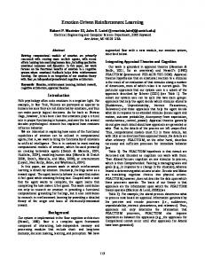
4. Experimental Results 4.1. Direct v.s. Indirect Methods: First Set-up We compared the performance of direct and indirect methods by the total (life time) profits obtained by the output policies, evaluated using the simulation model estimated from the same data. Figure 4 shows the total profits obtained by the direct (sarsa) and indrect methods, plotted as a function of the number of value iterations performed. The plots were obtained by averaging over 4 runs. Both the direct and indirect methods used as training data a subsample consisting of 10 thousand episodes, giving rise to 160 thousand event data. (The first 6 campaigns in each episode were discarded, due to lack of information regarding some of the temporal features.) The total profits are obtained us-

Direct(sarsa) error bars Indirect error bars

340000

320000

350000 profits

profits

Direct(sarsa) error bars Indirect error bars

400000

300000

300000

280000 250000 260000 200000 0

1

2

3 iterations

4

5

6

0

1

2

3 iterations

4

5

6

Figure 4. Total profits obtained by Direct and Indirect Methods in Experiment 1.

Figure 5. Total profits obtained by Direct and Indirect Methods in Experiment 2.

ing the simulation model as described in the previous section, and totaled over 20 campaigns. The error bars shown in the graph are the standard errors calculated from the total profits obtained in the four independent runs, namely

performed with restricted attention, the performance of the indirect method degrades significantly. It seems to support the thesis that, in practical situations in which not all the relevant features are available for analysis, the direct methods are more likely to generate more reliable policies.

=

rP

n i=1 (Pi

P )2 =n n

1

(6)

where Pi is the total profit obtained in the i-th run, P is the average total profit, and n is the number of runs (4 in this case). As one can see in Figure 4, in Experiment 1 in which the learning algorithms are given access to all features that characterize customer behavior, the indirect method performs better than the direct method. Recall that the above evaluation is conducted using a simulation model trained using the same features and is very closely mirrored by the internal simulation model used during learning of the indirect model, giving the indirect method an unfair advantage over the direct method. The direct method learned using only the original data set, which was generated presumably by a significantly different process in the real world.

4.2. Direct v.s. Indirect Methods: Second Set-up We also compared the total (life time) profits obtained by the direct and indirect methods in the second set-up. The two methods were again run on training data consisting of 10 thousand episodes, or 160 thousand event data. The episode data were generated using a simulator, using a policy that was obtained by the Base method, one that tries to maximize the immediate rewards. The results of these experiments are shown in Figure 5. These plots were obtained by averaging over 6 runs. As one can see in the graph, these results exhibit a rather striking contrast from the results in the first set-up. When learning is

4.3. Effect of Semi-direct Methods The performance of the semi-direct methods was compared against that of direct and semi-direct methods in the second set-up. The semi-direct method was run, performing sampling from a larger data set containing 50 thousand episodes, corresponding to 800 thousand event data, generated again using the same simulator. This is because the situation we suppose for the semi-direct methods is when we have abandunce of training data, and not all of them can be used in each iteration of the value iteration in the interest of computational efficiency. It started with the same number (10 thousand) of episode data, corresponding to 160 thousand event data, sampled from this larger data in the initial iteration, and in the subsequent iterations selectively sampled event data from randomly selected sub-episodes containing 320 thousand events. We note that it used training data of comparable size to the direct and indirect methods in these subsequent iterations, by the nature of its selective sampling strategy. Figure 6 shows the total profits obtained by two semidirect methods, as well as by the direct (sarsa) and indirect methods (averaged over 6 runs). The results indicate that, while the profitability of the policies output by the semidirect methods can become more unstable as the number of value iterations increases, well-performing policies can be obtained at earlier stages of value iteration. While CPU time used by the respective methods would be a more direct measure of computation time, it is also sensitive to the exact im-

Direct(sarsa) error bars Indirect error bars Semi-direct error bars

400000

profits

350000

300000

250000

200000 0

1

2

3 iterations

4

5

6

Figure 6. Total profits obtained by Direct, Indirect and Semi-direct Methods in Experiment 2.

plementation details, including the scalability properties of the base method. The data size is almost always a dominant factor in determining the computation time of the training process, and is a more robust measure. Since comparable data sizes were used by the respective methods, one can see that the semi-direct methods can be quite effective in reducing the computational requirement for obtaining policies of comparable profitability.

5. Conclusions We proposed and evaluated a series of reinforcement learning methods for sequential targeted marketing. Our experimental results verify our initial premise that, in this application domain, direct methods of reinforcement learning are better suited than indirect methods. We also demonstrated that the “semi-direct” methods can be effective in reducing the computational burden. Our experiments were admittedly preliminary in nature. In the future, we plan to verify these claims in real world applications.

6. Acknowledgments We thank Fateh Tipu for his help in carrying out our experiments.

References [1] C. Apte, E. Bibelnieks, R. Natarajan, E. Pednault, F. Tipu, D. Campbell, and B. Nelson. Segmentation-based modeling for advanced targeted marketing. In Proceedings of the Seventh ACM SIGKDD International Conference on Knowledge Discovery and Data Mining (SIGKDD), pages 408– 413. ACM, 2001.

[2] S. D. Bay. UCI KDD archive. Department of Information and Computer Sciences, University of California, Irvine, 2000. http://kdd.ics.uci.edu/. [3] D. P. Bertsekas and J. N. Tsitsiklis. Neuro-Dynamic Programming. Athena Scientific, 1996. [4] P. Domingos. MetaCost: A general method for making classifiers cost sensitive. In Proceedings of the Fifth International Conference on Knowledge Discovery and Data Mining, pages 155–164. ACM Press, 1999. [5] C. Elkan. The foundations of cost-sensitive learning. In Proceedings of the Seventeenth International Joint Conference on Artificial Intelligence, Aug. 2001. [6] W. Fan, S. J. Stolfo, J. Zhang, and P. K. Chan. AdaCost: misclassification cost-sensitive boosting. In Proc. 16th International Conf. on Machine Learning, pages 97–105. Morgan Kaufmann, San Francisco, CA, 1999. [7] L. P. Kaelbling, M. L. Littman, and A. W. Moore. Reinforcement learning: A survey. Journal of Artificial Intelligence Research, 4, 1996. [8] D. D. Margineantu and T. G. Dietterich. Bootstrap methods for the cost-sensitive evaluation of classifiers. In Proc. 17th International Conf. on Machine Learning, pages 583– 590. Morgan Kaufmann, San Francisco, CA, 2000. [9] R. Natarajan and E. Pednault. Segmented regression estimators for massive data sets. In Second SIAM International Conference on Data Mining, Arlington, Virginia, 2002. to appear. [10] E. Pednault, N. Abe, B. Zadrozny, H. Wang, W. Fan, and C. Apte. Sequential cost-sensitive decision making with reinforcement learning. In Proceedings of the Eighth ACM SIGKDD International Conference on Knowledge Discovery and Data Mining. ACM Press, 2002. To appear. [11] G. A. Rummery and M. Niranjan. On-line q-learning using connectionist systems. Technical Report CUED/FINFENG/TR 166, Cambridge University Engineering Departement, 1994. Ph.D. thesis. [12] R. S. Sutton and A. G. Barto. Reinforcement Learning: An Introduction. MIT Press, 1998. [13] P. Turney. Cost-sensitive learning bibliography. Institute for Information Technology, National Research Council, Ottawa, Canada, 2000. http://extractor.iit.nrc.ca/ bibliographies/cost-sensitive.html. [14] X. Wang and T. Dietterich. Efficient value function approximation using regression trees. In Proceedings of the IJCAI Workshop on Statistical Machine Learning for Large-Scale Optimization, 1999. [15] C. J. C. H. Watkins. Learning from Delayed Rewards. PhD thesis, Cambridge University, Cambridge, 1989. [16] C. J. C. H. Watkins and P. Dayan. Q-learning. Machine Learning, 8:279–292, 1992. [17] B. Zadrozny and C. Elkan. Learning and making decisions when costs and probabilities are both unknown. In Proceedings of the Seventh International Conference on Knowledge Discovery and Data Mining, 2001.