Sep 4, 2008 - 2005, Ferré and Villa 2006, Li and Yin 2008b] and solves the eigen- ... terms of a testing problem [Schott 1994, Ferré 1998, Bura and Cook ...
Consistency of regularized sliced inverse regression for kernel models Qiang Wu, Feng Liang, and Sayan Mukherjee∗ September 4, 2008
Abstract We develop an extension of the sliced inverse regression (SIR) framework for dimension reduction using kernel models and Tikhonov regularization. The result is a numerically stable nonlinear dimension reduction method. We prove consistency of the method under weak conditions even when the reproducing kernel Hilbert space induced by the kernel is infinite dimensional. We illustrate the utility of this approach on simulated and real data. Keywords: Dimension reduction, sliced inverse regression, kernel methods, regularization
∗
Qiang Wu and Sayan Mukherjee are members of the Departments of Statistical Science and Computer Science
and Institute for Genome Sciences & Policy, Duke University, Durham, NC 27708; Feng Liang is a member of the Department of Statistics, University of Illinois at Urbana-Champaign, IL 61820
1
1 Introduction The goal of dimension reduction in the standard regression/classification setting is to summarize the information in the p-dimensional predictor variable X relevant to predicting the univariate response variable Y . The summary S(X) should have d ≪ p variates and ideally
should satisfy the following conditional independence property Y ⊥⊥ X | S(X).
(1)
Thus any inference of Y involves only the summary statistic S(X) which is of much lower dimension than the original data X. Linear methods for dimension reduction focus on linear summaries of the data, that is, S(X) = (β1T X, . . . , βdT X). The d-dimensional subspace, S = span(β1 , ..., βd ), is defined
as the effective dimension reduction (e.d.r.) space in Li [1991] since S summaries all the
information we need to know about Y . A key result in Li [1991] is that under some mild
conditions the e.d.r. directions {βj }dj=1 correspond to the eigenvectors of the matrix T = [cov(X)]−1 cov[E(X|Y )]. Thus the e.d.r. directions or subspace can be estimated via an eigenanalysis of matrix T , which is the foundation of the sliced inverse regression algorithm proposed by Li [1991] and Duan and Li [1991]. Further developments include sliced average variance estimation [Cook and Weisberg 1991]. Recently this framework was extended to the high-dimensional setting where there are more covariates p than observations n in Li et al. [2007]. A common premise held in high-dimensional data analysis is that the intrinsic structure of data is in fact low dimensional, for example the data is concentrated on a manifold. Linear methods such as SIR often fail to capture this nonlinear low-dimensional structure. However, often there exists a nonlinear embedding of the data into a Hilbert space where a linear method can capture the low-dimensional structure. If projections onto this low-dimensional structure can be computed by inner products in this Hilbert space, kernel methods [Sch¨olkopf et al. 1997, Sch¨olkopf and Smola 2002] can be used to obtain simple and efficient algorithms. The basic idea in applying kernel methods is the application of a linear algorithm to the data mapped into a feature space induced by the kernel function. Since the embedding is nonlinear, linear directions in the feature space correspond to nonlinear directions in the original data space. Nonlinear extensions of some classical linear dimensional reduction methods using this approach are kernel principle component analysis [Sch¨olkopf et al. 1997] and kernel independent correlation analysis [Bach and Jordan 2002]. This idea was applied to SIR in Wu [2008] resulting in the kernel sliced inverse regression (KSIR) method which allows for the estimation of nonlinear e.d.r. directions.
2
There are numeric, algorithmic, and conceptual subtleties in a direct application of this kernel idea to SIR. If the kernel function is infinite dimensional, the embedding induced by the kernel function maps a point in the p-dimensional covariate space into an infinite dimensional Hilbert space, then T is an operator and is not well defined. In addition, for infinite or highdimensional feature spaces an empirical estimate of T based from observations is often illconditioned and results in computational instability. We seek to overcome these difficulties by proposing a modified version of KSIR that incorporates a Tikhonov regularization term. The method is stated as an eigen-decomposition problem as well as a least squares problem in Section 3. Addition of this regularization term has both theoretical and practical implications. The theoretical contribution is a proving asymptotic consistency of the e.d.r. estimates and with a rate of O(n1/4 ) under stated conditions, see Section 4. The practical contribution is empirical evidence that addition of the regularization term improves predictive accuracy, see Section 5.
2 Mercer kernels and nonlinear e.d.r. directions The extension of SIR to use kernels is based on properties of reproducing kernel Hilbert spaces (RKHS) and in particular Mercer kernels [Mercer 1909]. Given predictor variables X ∈ X ⊆ Rp , a Mercer kernel is a continuous, positive, semi-
definite function k(·, ·) : X × X → R with the following spectral decomposition X k(x, z) = λj φj (x)φj (z), j
where {φj } are the eigenfunctions and {λj } are the corresponding non-negative, non-increasing
eigenvalues. An important property of Mercer kernels is that each kernel k uniquely corresponds to a reproducing kernel Hilbert space (RKHS) X X H = f f (x) = aj φj (x) with aj 2 /λj < ∞ , j∈Λ
(2)
j∈Λ
where the cardinality of Λ := {j : λj > 0} is the dimension of the RKHS which may be
infinite [Mercer 1909, Ko¨ nig 1986].
The key idea is given a Mercer kernel there exists a unique map or embedding φ from X
to a Hilbert space defined by the eigenvalues and eigenfunctions of the kernel. The map takes the form φ(x) =
�p
λ1 φ1 (x),
p
λ2 φ2 (x), . . . ,
q
� λ|Λ| φ|Λ| (x) .
(3)
The Hilbert space induced by this map with the standard inner product k(x, z) = hφ(z), φ(z)i
is isomorphic to the RKHS (2) and we will denote both these Hilbert spaces as H [Ko¨ nig 1986]. In the case where k is infinite dimensional, φ : X → ℓ2 .
3
The random variable X ∈ X induces a random element φ(X) in the RKHS. Throughout
this paper we will use Hilbert space valued random variables so we now recall some basic
facts. Let Z be a random element in H with EkZk < ∞, where k · k denotes the norm in
H induced by its inner product h·, ·i. The expectation E(Z) is defined to be an element in H,
satisfying ha, E(Z)i = Eha, Zi, for all a ∈ H. If EkZk2 ≤ ∞, then the covariance operator of Z is defined as E[(Z − EZ) ⊗ (Z − EZ)], where
(a ⊗ b)f = hb, f ia for any f ∈ H. Let P denote the measure for random variable X. Throughout we assume the following
conditions.
Assumption 1. 1. For all x ∈ X , k(x, ·) is P-measurable. 2. There exists M > 0 such that x ∈ X , k(X, X) ≤ M almost surely (a.s.) with respect to P.
3. H is separable. Under Assumption 1, the random element φ(X) has a well-defined mean and covariance operator because kφ(x)k2 = k(x, x) is bounded (a.s.). Without loss of generality, we assume Eφ(X) = 0 where 0 is the vector of zeros in H. The boundedness also implies that the covari-
ance operator Σ = E[φ(X) ⊗ φ(X)] is compact and has the following spectral decomposition Σ=
∞ X i=1
wi ei ⊗ ei ,
(4)
where wi and ei ∈ H are the eigenvalues and eigenfunctions, respectively.
We assume the following model for the relationship between Y and X, � Y = F hβ1 , φ(X)i, . . . , hβd , φ(X)i, ε ,
(5)
with βj ∈ H and the distribution of ε is independent of X. This model implies that the
response variable Y depends on X only through a d-dimensional summary statistic � S(X) = hβ1 , φ(X)i, . . . , hβd , φ(X)i .
Although S(X) is a linear summary statistic in H, it extracts nonlinear features in the space
of the original predictor variables X. We call {βj }dj=1 the nonlinear e.d.r. directions, and
S = span(β1 , . . . , βd ) the nonlinear e.d.r. space. The following proposition [Wu 2008] extends
the theoretical foundation of SIR to this nonlinear setting.
4
Proposition 1. Assume the following linear design condition for H that for any f ∈ H, there
exists a vector b ∈ Rd such that
�T E[hf, φ(X)i|S(X)] = bT S(X), with S(X) = hβ1 , φ(X)i, . . . , hβd , φ(X)i .
(6)
Then for the model specified in equation (5) the inverse regression curve E[φ(X)|Y ] is contained in the span of (Σβ1 , . . . , Σβd ), where Σ is the covariance operator of φ(X). Proposition 1 is a straightforward extension of the multivariate case in Li [1991] to a Hilbert space or a direct application of the functional SIR setting in Ferr´e and Yao [2003]. Although the linear design condition (6) may be difficult to check in practice, it has been shown that such a condition usually holds approximately in a high-dimensional space [Hall and Li 1993], An immediate consequence of this proposition is that nonlinear e.d.r. directions are the eigenvectors corresponding to the largest eigenvalues of the following generalized eigen-decomposition problem Γβ = λΣβ,
where Σ = cov[φ(X)],
Γ = cov[E(φ(X)|Y )],
(7)
or equivalently from an eigenanalysis of the operator T = Σ−1 Γ. In the infinite dimensional case a technical difficulty arises since the operator Σ−1 =
∞ X i=1
wi−1 ei ⊗ ei
is not defined on the entire Hilbert space H. So for the operator T to be well-defined, we
need to show that the image of Γ is indeed in the range of Σ−1 . A similar issue also arose in
the analysis of dimension reduction and canonical analysis for functional data [He et al. 2003, Ferr´e and Yao 2005]. In these analyses, extra conditions are needed for operators like T to be well-defined. In KSIR this issue is resolved automatically by the linear design condition and extra conditions are not required as stated by the following Theorem, see Appendix A for the proof. Theorem 1. Under Assumption 1 and the linear design condition (6) in Proposition 1 the following hold: (i) The the operator Γ is of finite rank dΓ ≤ d. Consequently, it is compact and has the following spectral decomposition
Γ=
dΓ X i=1
τ i ui ⊗ ui ,
(8)
where τi and ui are the eigenvalues and eigenvectors, respectively. Moreover, ui ∈ range(Σ) for all i = 1, . . . , dΓ .
5
(ii) The eigen-decomposition problem (7) is equivalent to the eigenanalysis of the operator T , which takes the following form T =
dΓ X i=1
τi ui ⊗ Σ−1 (ui ).
3 Regularized kernel sliced inverse regression The discussion in Section 2 implies that nonlinear e.d.r. directions can be retrieved by applying the original SIR algorithm in the feature space induced by the Mercer kernel. There are some fundamental computational challenges to this idea such as estimating a an infinite dimensional covariance operator and the fact that the feature map is often difficult or impossible to compute for many kernels. We address these issues by working with inner products of the feature map and adding a Tikhonov regularization term to kernel SIR. We also provide a least squares formulation of this problem which enables us to select the regularization parameter via crossvalidation.
3.1 Estimating the nonlinear E.D.R. directions Given n observations {(x1 , y1 ), ..., (xn , yn )} our objective is to obtain an estimate of the e.d.r. directions (βˆ1 , ..., βˆd ). We first formulate a procedure almost identical to the standard SIR procedure except that it operates in the feature space H. This highlights the immediate relation
between the SIR and KSIR procedures.
1. Without loss of generality we assume that the mapped predictor variables are mean zero Pn i=1 φ(xi ) = 0. The sample covariance is estimated by n
X ˆ= 1 Σ φ(xi ) ⊗ φ(xi ) n i=1
2. Bin the Y variables into H slices G1 , . . . , GH and compute mean vectors of the corresponding mapped predictor variables for each group 1 X φ(xi ), h = 1, . . . , H, ψh = nh i∈Gh
Compute the sample between-group covariance matrix ˆ= Γ
H X nh h=1
n
ψh ⊗ ψh .
3. Estimate the SIR directions βˆj by solving the generalized eigen-decomposition problem ˆ = λΣβ. ˆ Γβ
6
(9)
This procedure is computationally impossible if the RKHS is infinite dimensional or the feature map cannot be computed. However, the the model given in (5) requires not the e.d.r. directions but only the projection onto these directions, that is, the d summary statistics v1 = hβ1 , φ(X)i, . . . , vd = hβd , φ(X)i, which we call the KSIR variates. The KSIR variates can be efficiently computed and require only the kernel k(·, ·), not the map φ.
The key quantity in this alternative formulation is the centered gram matrix K defined by
the kernel k(·, ·) where Kij
¯ φ(xj ) − φi ¯ = hφ(xi ) − φ, n n n 1X 1 X 1X k(xi , xj ). k(xi , xj ) − k(xi , xj ) + 2 = k(xi , xj ) − n n n j=1
i=1
i,j=1
Note that the rank of K is less than n, so K is always singular. Given the centered gram matrix K, the following generalized eigen-decomposition problem can be used to compute the KSIR variates KJKc = λK 2 c,
(10)
where c denotes the n-dimensional generalized eigenvector, and J denotes a n × n matrix with
Jij = 1/nm if i, j are in the m-th group consisting of nm observations and zero otherwise.
The following proposition states that two eigen-decomposition problems, (10) and (9), are equivalent in the recover the same KSIR covariates (v1 , .., vd ). Proposition 2. Given observations {(x1 , y1 ), ..., (xn , yn )}, let (βˆ1 , . . . , βˆd ) and (ˆ c1 , . . . , cˆd ) denote the generalized eigenvectors of (10) and (9), respectively. Then for any x ∈ X and
j = 1, . . . , d, the following holds
hβˆj , φ(x)i = cˆTj Kx ,
�T Kx = k(x, x1 ), ...., k(x, xn ) ,
ˆ is invertible. When Σ ˆ is not invertible, the conclusion still holds modulo the null provided Σ ˆ space of Σ. This result was proven in Wu [2008], in which the algorithm was further reduced to solving JKc = λKc by canceling K from both sides of (10). This may cause some problems since K is singular so we work with the original symmetric form (10), which also results in a simple interpretation of the regularization approach we now introduce.
7
3.2 Regularization and stability The eigen-decomposition in equation (10) will often be ill-conditioned resulting in over-fitting as well as numerically unstable estimates of the e.d.r. space. This can be addressed by either ˆ or by adding a regularization thresholding eigenvalues of the estimated covariance matrix Σ term to (10). We introduce the following regularization: KJKc = λ(K 2 + n2 sI)c,
(11)
where s is a tuning parameter. This results in robust estimates of the e.d.r. space and improved predictive accuracy. The following proposition, see Appendix B for proof, states that solving the generalized eigen-decomposition problem (11) is equivalent to finding the eigenvectors of ˆ 2 + sI)−1 Σ ˆ Γ. ˆ (Σ
(12)
Proposition 3. Let cˆj be the eigenvectors of (11) and βˆj be the eigenvectors of (12), then the following holds for the regularized KSIR covariates vˆj = cˆTj [k(x, x1 ), . . . , k(x, xn )] = hβˆj , φ(x)i. Ridge type regularization is an alternative widely used in both linear SIR and functional SIR [Zhong et al. 2005, Ferr´e and Villa 2006, Li and Yin 2008b] and solves the eigen-decomposition ˆ = λ(Σ ˆ + sI)β. Γβ
(13)
It was shown in Bernard-Michel et al. [2008] that Tikhonov regularization is more efficient. To close, we remark that KSIR is computationally advantageous even for the case of linear models when p ≫ n due to the fact that the eigen-decomposition problem is for n × n matrices rather than the p × p matrices in the standard SIR formulation.
3.3 Least square formulation The generalized eigen-decomposition for linear SIR can be written as a least square formulation [Cook 2004, Li and Yin 2008b]. The advantage of the this formulation is that a greater variety of regularization or shrinkage models can be applied such as ℓ1 penalties. In addition, classical techniques such as generalized cross validation can be used to select the regularization parameter. We can also formulate regularized KSIR as a least square problem. Denote zi as the i-th column of K. This corresponds to thinking of the matrix K as a data matrix of n observations in a n-dimensional space. For this new data matrix, we can estimate the covariance of the inverse regression as ˆ= Γ
H X nh h=1
1 Z¯h Z¯hT = KJK, n n
8
where Z¯h =
1 nh
P
i∈Gh zi
and the e.d.r. directions can be estimated by solving the eigen-
decomposition problem in equation (10). Informally, this perspective views KSIR as linear SIR in an n-dimensional space. This formulation and arguments in Cook [2004], Li and Yin [2008b] lead to the following least square penalty G(C, A) =
H X
nh
Z¯h − 1 K 2 Cah 2 , n n h=1
where C = (c1 , c2 , . . . , cd ) ∈ Rn×d and A = (a1 , . . . , aH ) ∈ Rd×H . By arguments from
Li and Yin [2008b] the top d eigenvectors for the KSIR algorithm (10) can be computed by minimizing G(C, A) with respect to C and A. By the same argument regularized KSIR (11) can be solved by minimizing the following penalized least square loss functional with respect to C and A � Gs (C, A) = G(C, A) + ns vec(CA)T D ⊗ n1 K 2 vec(CA)
where D = diag( nn1 , . . . , nnH ) and vec(·) is a matrix operation that stacks all columns of a matrix. Once either A or C is fixed the above functional is a regularized least square problem, suggesting iteratively solving for A and C. Given an estimate Cˆ = (ˆ ci , ..., cˆd ) the solution coincides with the formula as given by equation (11). One motivation for the least square formulation in Li and Yin [2008a] is selection of the regularization parameter by a generalized cross-validation criterion. The criterion suggested by Li and Yin [2008a] can be written as follows for the regularized KSIR model GCV =
˜ k(InH − Qs )W 1/2 Zk nH[1 − trace(Qs )/nH]2
where W = D ⊗ In , Z˜ = vec(Z¯1 , . . . , Z¯H ), and � � ˆ AˆT )−1 AD ˆ 1/2 ⊗ Qs = D 1/2 AˆT (AD
2 1 n2 K(K
� + n2 sIn )K .
For linear SIR there are many methods to estimate the correct number e.d.r. directions in terms of a testing problem [Schott 1994, Ferr´e 1998, Bura and Cook 2001, Zhu et al. 2006]. Considering KSIR as linear in the gram matrix might allow us to select the correct number of e.d.r. directions using the same tests.
4 Consistency of regularized KSIR In this section, we prove the asymptotic consistency of the e.d.r. directions estimated by KSIR and provide conditions under which the rate of consistency is Op (n−1/4 ). Our result also implies consistency for functional SIR with Tikhonov regularization. An important observation
9
from the proof is that the rate of convergence of the e.d.r. directions depends on the contribution of the smaller principal components. The rate can be arbitrarily slow if the e.d.r. space depends heavily on eigenvectors corresponding to small eigenvalues of the covariance operator. Note that various consistency results are available for linear SIR [Hsing and Carroll 1992, Saracco 1997, Zhu and Ng 1995]. These results hold only for the finite dimensional setting and cannot be adapted to KSIR where the RKHS is often infinite dimensional. Consistency of functional SIR has also been studied before. In Ferr´e and Yao [2003] a thresholding method is considered, which selects a finite number of eigenvectors and uses results from finite rank operators. Their proof of consistency requires stronger and more complicated conditions than ours. The consistency for functional SIR with ridge regularization is proven in Ferr´e and Villa [2006], but it is of a weaker form than our result. This suggests that either there is a theoretical advantage for Tikhonov regularization over ridge regression or the previous consistency results for functional SIR can be improved. The following theorem states the formal consistency result. √ Theorem 2. Assume Ek(X, X)2 < ∞, limn→∞ s(n) = 0 and limn→∞ s n = ∞, then hβˆj , φ(·)i − hβj , φ(·)i = op (1), j = 1, ..., dΓ ,
where dΓ is the rank of Γ, hβj , φ(·)i is the projection onto the j-th e.d.r., and hβˆj , φ(·)i is the projection onto the j-th e.d.r. as estimated by regularized KSIR.
Γ If the e.d.r. directions {βj }dj=1 depend only on a finite number of eigenvectors of the co-
variance operator Σ the rate of convergence is O(n−1/4 ).
This theorem is a direct corollary of the following theorem which is proven in Appendix C. Theorem 3. First define for N ≥ 1 the projection operator and its complement ΠN =
N X i=1
ei ⊗ ei ,
Π⊥ N = I − ΠN =
∞ X
i=N +1
ei ⊗ ei ,
where {ei }∞ i=1 are the eigenvectors of the covariance operator Σ as defined in (4), with the
corresponding eigenvalues denoted by wi .
Assume Ek(X, X)2 < ∞. For each N ≥ 1 the following holds ˆ + sI)−1 Σ ˆΓ ˆ − T kHS = Op k(Σ
�
1 √
s n
�
� dΓ � X s ⊥ uj )k + kΠN (˜ uj )k + 2 kΠN (˜ wN j=1
dΓ where u ˜j = Σ−1 uj and {uj }i=1 are the eigenvectors of Γ as defined in (8). √ If s = s(n) satisfy s → 0 and s n → ∞ as n → ∞, then
ˆ + sI)−1 Σ ˆΓ ˆ − T kHS = op (1). k(Σ
10
(14)
5 Application to simulated and real data In this section we compare classical sliced inverse regression (SIR), regularized sliced inverse regression (RSIR) as in (13), kernel sliced inverse regression (KSIR), and regularized kernel sliced inverse regression (RKSIR). The comparisons are used to address two questions: (1) does regularization improve the performance of kernel sliced inverse regression, and (2) in real data does the nonlinearity of kernel sliced inverse regression improve predictive performance. We show using three examples that regularization does help with estimating the e.d.r. directions and the nonlinearity introduced by the kernel versions can make a dramatic difference in terms of predictive accuracy.
5.1 Importance of nonlinearity and regularization This example illustrates that both the nonlinearity and regularization of RKSIR can significantly improve prediction accuracy. The regression model has ten predictor variables X = (X1 , ..., X10 ) and a univariate response specified by Y =
! ! 5 10 1X 1X 1+ sin(π Xi ) 1+ sin(π Xi ) + ε, 5 5 i=1
i=6
where each of the ten dimensions are uniform in [−1.1], Xi ∼ U [−1, 1] for i = 1, ..., 10, and the noise is normal ε ∼ N (0, .12 ).
We examined the predictive accuracy as a function of the number of e.d.r. directions used
in a Gaussian kernel regression model the bandwith parameter of the Gaussian was set to the median of pairwise distances. We compared the performance of using SIR, KSIR, and RKSIR to compute the e.d.r. directions in this procedure. We used a training set of 100 observations to compute the e.d.r. directions and fit the nonlinear regression model. We then used an independent test set of 2000 observations to compute the mean square error of the regression model estimated. For both KSIR and RKSIR we used an additive Gaussian kernel k(x, z) =
d X j=1
� exp −(xj − zj )2 /2σ 2 .
The regularization parameter in RKSIR was set by cross-validation. Figure 1 displays the accuracy of the procedure as a function of the number of e.d.r. directions for the three methods. The result for SIR shows that linear directions do not capture the predictive structure in this data this structure is distributed across all ten e.d.r. directions. The result for KSIR illustrates that by adding the nonlinearity most of the predictive structure is captured in the first e.d.r. direction. However, this direction is far from optimal. For RKSIR
11
the first e.d.r. direction contains almost all of the predictive structure and adding regularization has greatly improved accuracy.
5.2 Effect of regularization This example illustrates how regularization has an effect on the performance of KSIR as a function of the anisotropy of the predictors. The regression model has ten predictor variables X = (X1 , ..., X10 ) and a univariate response specified by Y = X1 + X22 + ε,
ε ∼ N (0, 0.12 ),
(15)
where X ∼ N (0, ΣX ) and ΣX = Q∆Q with Q a randomly chosen orthogonal matrix and
∆ = diag(1θ , 2θ , . . . , 10θ ). We will see increasing the parameter θ ∈ [0, ∞) increases the anisotropy of the data which amplifies the importance of correctly inferring the top e.d.r. directions. For this model it is known that SIR will not accurately infer the e.d.r. space since only the the first variable X1 will be identified. For this reason we focus on the comparison of KSIR and RKSIR in this example. If we use a second order polynomial kernel k(x, z) = (1 + xT z)2 this corresponds to the feature space Φ(X) = {1, Xi , (Xi Xj )i≤j } i, j = 1, ..., 10. In this feature space X1 +X22 can be captured in one e.d.r. direction. Thus using the polynomial kernel a one dimensional e.d.r. space should contain all the predictive information. Ideally the first KSIR variate v = hβ1 , φ(X)i should be equivalent to X1 + X22 modulo
shift and scale
v − Ev ∝ X1 + X22 − E(X1 + X22 ). So for this example given estimates of KSIR variates at the n data points {ˆ vi }ni=1 = {hβˆ1 , φ(xi )i}ni=1
the error of the first e.d.r. direction can be measured from the following optimization problem n �2 1X vˆi − Ev − a(xi,1 + x2i,2 − E(X1 + X22 )) a∈R n i=1 n �2 1X = min vˆi − (a(xi,1 + x2i,2 ) + b) . a,b∈R n
error = min
i=1
We drew 200 observations from the model specified in (15). We then applied the two dimension reduction methods KSIR and RKSIR. The mean and standard errors of 100 repetitions of this procedure are reported in Figure 2. The result shows that KSIR becomes more and more unstable as θ increase and regularization helps to reduce this instability.
12
5.3 Importance of nonlinearity and regularization in real data When SIR is applied to classification problems, it is equivalent to a Fisher discriminant analysis. For the case of multiclass classification it is natural to use SIR and consider each class as a slice. Kernel forms of Fisher discriminant analysis (KFDA) [Baudata and Anouar 2000] have been used to construct nonlinear discriminant surfaces and regularization has improved performance of KFDA [Kurita and Taguchi 2005]. In this example we show that this idea of adding a nonlinearity and a regularization term improves predictive accuracy in a real multiclass classification data set, the classification of handwritten digits. The MNIST data set (Y. LeCun, http://yann.lecun.com/exdb/mnist/), contains 60, 000 images of handwritten digits {0, 1, 2, ..., 9} as training data and 10, 000 images as test data. Each image consists of p = 28 × 28 = 784 gray-scale pixel intensities. It is commonly believed that there is clear nonlinear structure in this 784 dimensional space.
We compared RSIR, KSIR, and RKSIR on this data to examine the effect of regularization and nonlinearity. Each draw of the training set consisted of 100 observations of each digit. We then computed the top 10 e.d.r. directions using these 1000 observations and 10 slices, one for each digit. We projected the 10, 000 test observations onto the e.d.r. directions and used a k-nearest neighbor (kNN) classifier with k = 5 to classify the test data. The accuracy of the kNN classifier without dimension reduction was used as a baseline. For KSIR and RKSIR we used a Gaussian kernel with the bandwith parameter set as the median pairwise distance between observations. The regularization parameter was set by cross-validation. The mean and standard deviation of the classification accuracy over 100 iterations of this procedure is reported in Table 1. The first interesting observation is that linear dimension reduction does not capture discriminative information as the classification accuracy without dimension reduction is better. Nonlinearity does increase classification accuracy and coupling regularization with nonlinearity increases accuracy more. This improvement is dramatic for 2, 3, 5, and 8.
6 Discussion The interest in manifold learning and nonlinear dimension reduction in both statistics and machine learning has led to a variety of statistical models and algorithms. However, most these methods are developed in the unsupervised learning framework. Therefore the estimated dimensions may not be optimal for regression models. Incorporating nonlinearity and regularization to inverse regression approaches results in a robust response driven nonlinear dimension reduction method. A least square formulation is also provided for parameter selection. There are some interesting relations between KSIR and functional SIR. In functional SIR,
13
the observable data are functions and the goal is to find linear e.d.r. directions for functional data analysis. In KSIR, the observable data are typically not functions but mapped into a function space in order to characterize nonlinear structures. This suggests computations involved in functional SIR can be simplified by a parametrization with respect to a RKHS or using a linear kernel in the parametrized function space. From a theoretical point of view, KSIR can be viewed as a special case of functional SIR as developed by Ferr´e and his coauthors in a series of papers [Ferr´e and Yao 2003, 2005, Ferr´e and Villa 2006].
Acknowledgments We acknowledge support of the National Science Foundation ( DMS-0732276 and DMS0732260) and the National Institutes of Health (P50 GM 081883). Any opinions, findings and conclusions or recommendations expressed in this work are those of the authors and do not necessarily reflect the views of the NSF or NIH.
References BACH , F. R. and J ORDAN , M. I. (2002). Kernel independent component analysis. Journal of Machine Learning Research 3 1–48. BAUDATA , G. and A NOUAR , F. (2000). Generalized discriminant analysis using a kernel approach. Neural Computation 12 2385–2404. B ERNARD -M ICHEL , C., G ARDES , L. and G IRARD , S. (2008). Gaussian regularized sliced inverse regression. Preprint. B LANCHARD , G., B OUSQUET, O. and Z WALD , L. (2007). Statistical properties of kernel principal component analysis. Mach. Learn. 66 259–294. B URA , E. and C OOK , R. D. (2001). Extending sliced inverse regression: the weighted chisquared test. J. Amer. Statist. Assoc. 96 996–1003. C HATELIN , F. (1983). Spectral Approximation of Linear Operators. Academic Press. C OOK , R. and W EISBERG , S. (1991). Disussion of li (1991). J. Amer. Statist. Assoc. 86 328–332. C OOK , R. D. (2004). Testing predictor contributions in sufficient dimension reduction. Ann. Statist. 32 1062–1092.
14
D UAN , N. and L I , K. (1991). Slicing regression: a link-free regression method. Ann. Stat. 19 505–530. F ERR E´ , L. (1998). Determining the dimension in sliced inverse regression and related methods. J. Amer. Statist. Assoc. 93 132–140. F ERR E´ , L. and V ILLA , N. (2006). Multilayer perceptron with functional inputs: an inverse regression approach. Scandinavian Journal of Statistics 33 807–823. F ERR E´ , L. and YAO , A. (2003). Funtional sliced inverse regression analysis. Statistics 37 475–488. F ERR E´ , L. and YAO , A. (2005). Smoothed functional inverse regression. Statist. Sinica 15 665–683. H ALL , P. and L I , K.-C. (1993). On almost linearity of low-dimensional projections from high-dimensional data. Ann. Statist. 21 867–889. ¨ H E , G., M ULLER , H. and WANG , J. (2003). Functional canonical analysis for square integrable stochastic processes. J. Multivariate Anal. 85 54–77. H SING , T. and C ARROLL , R. J. (1992). An asymptotic theory for sliced inverse regression. Ann. Statist. 20 1040–1061. K ATO , T. (1966). Perturbation Theory for Linear Operators. Springer-Verlag, Berlin, Heidelbert, New York. ¨ K ONIG , H. (1986). Eigenvalue distribution of compact operators, Operator Theory: Advances and Applications, vol. 16. Birkh¨auser, Basel, CH. K URITA , T. and TAGUCHI , T. (2005). A kernel-based fisher discriminant analysis for face detection. IEICE TRANS. INF. & SYST. E88CD 628–635. L I , K. (1991). Sliced inverse regression for dimension reduction (with discussion). J. Amer. Statist. Assoc. 86 316–342. L I , L., C OOK , R. and T SAI , C.-L. (2007). Partial inverse regression. Biometrika 94 615–625. L I , L. and Y IN , X. (2008a). Rejoinder to “a note on sliced inverse regression with regularizations” Preprint. L I , L. and Y IN , X. (2008b). Sliced inverse regression with regularizations. Biopmetrics 64 124–131.
15
M ERCER , J. (1909). Functions of positive and negative type and their connection with the theory of integral equations. Philosophical Transactions of the Royal Society, London A 209 415–446. S ARACCO , J. (1997). An asymptotic theory for sliced inverse regression. Comm. Statist. Theory Methods 26 2141–2171. ¨ S CH OLKOPF , B. and S MOLA , A. J. (2002). Learning with kernels. MIT Press, MA. ¨ ¨ S CH OLKOPF , B., S MOLA , A. J. and M ULLER , K. (1997). Kernel principal component analysis. In Artificial Neural Networks ICANN’97 (W. Gerstner, A. Germond, M. Hasler and J.-D. Nicoud, eds.), Springer Lecture Notes in Computer Science, vol. 1327, 583–588. Berlinpp. S CHOTT, J. R. (1994). Determining the dimensionality in sliced inverse regression. J. Amer. Statist. Assoc. 89 141–148. W U , H.-M. (2008). Kernel sliced inverse regression with applications on classification. Journal of Computational and Graphical Statistics Accepted. Z HONG , W., Z ENG , P., M A , P., L IU , J. S. and Z HU , Y. (2005). RSIR: regularized sliced inverse regression for motif discovery. Bioinformatics 21 4169–4175. Z HU , L., M IAO , B. and P ENG , H. (2006). On sliced inverse regression with high-dimensional covariates. J. Amer. Statist. Assoc. 101 630–643. Z HU , L. X. and N G , K. W. (1995). Asymptotics of sliced inverse regression. Statist. Sinica 5 727–736.
16
Appendix A: proof of Theorem 1 Under the assumption of Proposition 1, for each Y = y, E[φ(X)|Y = y] ∈ span{Σβi , i = 1, . . . , d}.
(16)
So the rank of Γ (i.e., the dimension of the image of Γ) is less than d. Since this implies Γ is compact, together with the fact it is symmetric and positive, there exist dΓ positive eigenvalues PΓ Γ Γ {τi }di=1 and eigenvectors {ui }di=1 such that Γ = di=1 τi ui ⊗ ui . Recall that for any f ∈ H,
Γf = hE[φ(X)|Y ], f i E[φ(X)|Y ] also belongs to span{Σβi , i = 1, . . . , d} ⊂ range(Σ) because of (16), so ui =
1 Γui ∈ range(Σ). τi
This proves (i). Since for each f ∈ H, Γf ∈ range(Γ), the operator T = Σ−1 Γ is well defined over the
whole space. Moreover, Tf = Σ
dΓ X i=1
hui , f iui
!
dΓ X = hui , f iΣ(ui ) = i=1
dΓ X i=1
Σ(ui ) ⊗ ui
!
f.
This proves (ii).
Appendix B: Proof of Proposition 3 We first prove the proposition for matrices to simplify notation we then extend the result to operators where dK is infinite and a matrix form does not make sense. Suppose Φ has the following SVD decomposition
Φ = U DV T = [u1 . . . udK ]
"
¯ d×d D
0(n−d)×d
# v1T 0(n−d)×(dK −d) ... = U ¯D ¯ V¯ T , 0(n−d)×(dK −d) vnT
(17)
¯ = [u1 , . . . , ud ], V¯ = [v1 , . . . , vd ], and D ¯ =D ¯ d×d is a diagonal matrix of dimension where U d ≤ n.
We need to show the KSIR variates vˆj = cTj [k(x, x1 ), . . . , k(x, xn )] = cTj ΦT Φ(x) = hΦcj , φ(x)i = hβj , φ(x)i.
17
It suffices to prove that if (λ, c) is a solution to (11), then (λ, β) is also a pair of eigenvalue and ˆ 2 + γI)−1 Σ ˆΓ ˆ and vice versa, where c and β is related by eigenvector of (Σ ¯U ¯ T β. β = Φc and c = V¯ D ˆ = Noting that facts Σ
1 T n ΦΦ ,
ˆ = Γ
1 T n ΦJΦ ,
¯ 2 V¯ T , the argument may and K = ΦT Φ = V¯ D
be made as follows: ˆ Γβ ˆ = λ(Σ ˆ 2 + γI)β ⇐⇒ ΦΦT ΦJΦT Φc = λ(ΦΦT ΦΦT Φc + n2 γΦc) Σ �
⇐⇒ ΦKJKc = λΦ(K 2 + n2 γ)c ⇐⇒ V¯ V¯ T KJKc = λV¯ V¯ T (K 2 + n2 γI)c
⇐⇒ KJKc = λ(K 2 + n2 γI)c.
�
Note the implication in the third step is necessary only in the =⇒ direction which is obtained ¯ −1 U ¯ T and using the facts U ¯T U ¯ = Id . For the last step, since by multiplying both sides V¯ D V¯ T V¯ = Id , we use the facts ¯ 2 V¯ T = V¯ D ¯ 2 V¯ T = K V¯ V¯ T K = V¯ V¯ T V¯ D and ¯ −1 U ¯ T β = V¯ D ¯ −1 U ¯ T β = c. V¯ V¯ T c = V¯ V¯ T V¯ D In order for this result to hold rigorously when the RKHS is infinite dimensional we need to formally define Φ, ΦT , and the SVD of Φ when dK is infinite. For the infinite Pn dimensional case, Φ is an operator from Rn to HK defined by Φv = i=1 vi φ(xi ) for
v = (v1 , . . . , vn )T ∈ Rn and ΦT is its adjoint, an operator from HK to Rn such that ¯ and U ¯ T are similarly ΦT f = (hφ(x1 ), f iK , . . . , hφ(x1 ), f iK )T for f ∈ HK . The notions U defined.
ˆ as a covariance operator. The above formulation of Φ and ΦT coincides the definition of Σ ˆ is less than n, it is compact and has the following representation: Since the rank of Σ ˆ= Σ
dK X i=1
σ ˆi ui ⊗ ui =
d X i=1
σi ui ⊗ ui
where d ≤ n is the rank and σ1 ≥ σ2 ≥ . . . ≥ σd > σd+1 = . . . = 0. This im¯ τi where U ¯ = plies each φ(xi ) lies in span(u1 , . . . , ud ) and hence we can write φ(xi ) = U (u1 , . . . , ud ) should be considered as an operator from Rd to HK and τi ∈ Rd . Denote by ¯ d×d = Υ = (τ1 , . . . , τn )T ∈ Rn×d. It is easy to check that ΥT Υ = diag(nσ1 , . . . , nσd ). Let D √ √ ¯ −1 . Then we obtain the SVD for Φ as Φ = U ¯D ¯ V¯ T diag( nσ1 , . . . , nσd ) and V¯ = ΥD which is well defined.
18
Appendix C: Proof of Consistency C.1 Preliminaries In order to prove Theorems 2 and Theorem 3 we use properties of Hilbert-Schmidt operators, covariance operators for Hilbert space valued random variables, and perturbation theory for linear operators. In this subsection we provide a brief introduction to them. For details see Kato [1966], Chatelin [1983], Blanchard et al. [2007] and references therein. Given a separable Hilbert space H of dimension pH , an linear operator L on H is said to
belong to the Hilbert-Schmidt class if
p
kLk2HS
=
H X
i=1
kLei k2H < ∞,
where {ei } is an orthogonal basis. The Hilbert-Schmidt class forms a new Hilbert space with norm k · kHS .
Given a bounded operator S on H, the operators SL and LS both belong to the Hilbert-
Schmidt class and the following holds
kSLkHS ≤ kSkkLkHS ,
kLSkHS ≤ kLkHS kSk
where k · k denotes the default operator norm kLf k2 . 2 f ∈H kf k
kLk2 = sup
Let Z be a random vector taking values in H satisfying EkZk2 < ∞. The covariance
operator
Σ = E[(Z − EZ) ⊗ (Z − EZ)], is self-adjoint, positive, compact, and belongs to Hilbert-Schmidt class. A well known result from perturbation theory for linear operators states that if a set of linear operators Tn converges to T in the Hilbert-Schmidt norm and the eigenvalues of T are nondegenerate, then the eigenvalues and eigenvectors of Tn converge to those of T with same rate or convergence as the convergence of the operators.
C.2 Proof of Theorem 3. We will use the following result from Ferr´e and Yao [2003] √ ˆ − ΣkHS = Op (1/ n) kΣ
and
√ ˆ − ΓkHS = Op (1/ n). kΓ
ˆ + sI)−1 Σ ˆ Γ. ˆ Also define To simply the notion, we denote by Tˆs = (Σ ˆ 2 + sI)−1 ΣΓ T1 = (Σ
and
19
T2 = (Σ2 + sI)−1 ΣΓ.
Then kTˆs − T kHS ≤ kTˆs − T1 kHS + kT1 − T2 kHS + kT2 − T kHS . For the first term observe that ˆ 2 + sI)−1 kkΣ ˆΓ ˆ − ΣΓkHS = Op kTˆs − T1 kHS ≤ k(Σ
�
1 √
s n
�
.
For the second term note that T1 =
dΓ X j=1
� � ˆ 2 + sI)−1 Σuj ⊗ uj τj (Σ
and
T2 =
dΓ X j=1
� τj (Σ2 + sI)−1 uj ⊗ uj .
Therefore kT1 − T2 kHS =
dΓ X j=1
� �
ˆ2 + sI)−1 − (Σ2 + sI)−1 Σuj . τj (Σ
Since uj ∈ range(Σ) there exists u ˜j such that uj = Σ˜ uj . Then � � � � ˆ 2 + sI)−1 Σ ˆ 2 − Σ2 (Σ2 + sI)−1 Σ2 u ˆ 2 + sI)−1 Σuj = (Σ ˜j . (Σ2 + sI)−1 − (Σ which implies dΓ X
ˆ2
ˆ2
ˆ2 + sI)−1 Σ2 k˜ uj k − Σ2 (Σ + sI)−1 Σ τj (Σ HS j=1� � 1 √ = Op . s n
kT1 − T2 k ≤
For the third term the following holds kT2 − T kHS = and for each j = 1, . . . , dΓ ,
dΓ X j=1
� τj (Σ2 + sI)−1 Σ − Σ−1 uj
k(Σ2 + sI)−1 Σuj − Σ−1 uj k ≤ k(Σ2 + sI)−1 Σ2 u ˜j − u ˜ k
! j ∞ 2
X w
j − 1 h˜ uj , ei iei = 2
s + wj i=1 ! 1/2 ∞ X s2 2 = h˜ uj , ei i (s + wi2 )2 i=1 !1/2 !1/2 ∞ N X X s h˜ uj , ei i2 + h˜ uj , ei i2 ≤ wN i=1 i=N +1 s ⊥ uj )k + kΠN (˜ uj )k. = 2 kΠN (˜ wN Combining these terms results in (14).
20
Since kΠ⊥ uj )k → 0 as N → ∞, consequently we have N (˜ kTˆs − T kHS = op (1) √ if s → 0 and s n → ∞.
If all the e.d.r. directions βi depend only on a finite number of eigenvectors of the covari-
ance operator, then there exist some N > 1 such that S ∗ = span{Σei , i = 1, . . . , N }. This implies
u ˜j = Σ−1 uj ∈ Σ−1 (S ∗ ) ⊂ span{ei , i = 1, . . . , N }. Therefore kΠ⊥ uj )k = 0. Let s = O(n−1/4 ) the rate is O(n1/4 ). N (˜
21
0.22
RKSIR KSIR SIR
0.2
0.18
0.16
Error
0.14
0.12
0.1
0.08
0.06
0.04
0.02
0
1
2
3
4
5
6
7
8
9
Number of e.d.r. directions
Figure 1: Mean square error on test data versus number of e.d.r. directions for the product of sines. The blue curve is a plot of the mean and standard error for SIR, the red curve is the same for RKSIR, and the green curve is for KSIR.
22
700
KSIR 600
RKSIR
Error rate
500
400
300
200
100
0 −0.5
0
0.5
1
1.5
2
Theta parameter Figure 2: Error in e.d.r. as a function of θ.
23
2.5
digit
RKSIR
KSIR
RSIR
kNN
0
0.0273 (0.0089) 0.0472 (0.0191) 0.0487 (0.0128) 0.0291 (0.0071)
1
0.0150 (0.0049) 0.0177 (0.0051) 0.0292 (0.0113) 0.0052 (0.0012)
2
0.1039 (0.0207) 0.1475 (0.0497) 0.1921 (0.0238) 0.2008 (0.0186)
3
0.0845 (0.0208) 0.1279 (0.0494) 0.1723 (0.0283) 0.1092 (0.0130)
4
0.0784 (0.0240) 0.1044 (0.0461) 0.1327 (0.0327) 0.1617 (0.0213)
5
0.0877 (0.0209) 0.1327 (0.0540) 0.2146 (0.0294) 0.1419 (0.0193)
6
0.0472 (0.0108) 0.0804 (0.0383) 0.0816 (0.0172) 0.0446 (0.0081)
7
0.0887 (0.0169) 0.1119 (0.0357) 0.1354 (0.0172) 0.1140 (0.0125)
8
0.0981 (0.0259) 0.1490 (0.0699) 0.1981 (0.0286) 0.1140 (0.0156)
9
0.0774 (0.0251) 0.1095 (0.0398) 0.1533 (0.0212) 0.2006 (0.0153)
average
0.0708 (0.0105) 0.1016 (0.0190) 0.1358 (0.0093) 0.1177 (0.0039)
Table 1: Mean and standard deviations for error rates in classification of digits.
24