Nonlinear Dimension Reduction with Kernel Sliced Inverse Regression

JOURNAL OF LATEX CLASS FILES, VOL. 6, NO. 1, JANUARY 2007

1

Nonlinear Dimension Reduction with Kernel Sliced Inverse Regression Yi-Ren Yeh, Su-Yun Huang, and Yuh-Jye Lee Abstract—Sliced inverse regression (SIR) is a renowned dimension reduction method for finding an effective low-dimensional linear subspace. Like many other linear methods, SIR can be extended to nonlinear setting via the “kernel trick”. The main purpose of this article is two-fold. We build kernel SIR in a reproducing kernel Hilbert space rigorously for a more intuitive model explanation and theoretical development. The second focus is on the implementation algorithm of kernel SIR for fast computation and numerical stability. We adopt a low rank approximation to approximate the huge and dense full kernel covariance matrix and a reduced singular value decomposition technique for extracting kernel SIR directions. We also explore kernel SIR’s ability to combine with other linear learning algorithms for classification and regression including multiresponse regression. Numerical experiments show that kernel SIR is an effective kernel tool for nonlinear dimension reduction and it can easily combine with other linear algorithms to form a powerful toolkit for nonlinear data analysis. Index Terms—dimension reduction, eigenvalue decomposition, kernel, reproducing kernel Hilbert space, singular value decomposition, sliced inverse regression, support vector machines.

✦

1

I NTRODUCTION

D

IMENSION reduction is an important topic in machine learning and data mining. The main demand comes from complex data analysis, data visualization and parsimonious modeling [1], [2]. Modern data are usually complex, high-dimensional and with nonlinear structures. A dimension reduction technique helps us to characterize the key data structure using only a few main features ranked by their importance. It thus provides a way for data visualization to gain better intuitive insights of the underlying data. The most popular dimension reduction method is probably the principal component analysis (PCA), which is an unsupervised method. In contrast, the sliced inverse regression (SIR) [3] extracts the dimension reduction subspace, called the effective dimension reduction (e.d.r.) subspace, based on the covariance matrix of input attributes inversely regressed on the responses. SIR can be viewed as a supervised companion of PCA for linear dimension reduction. SIR has won its reputation to perform well in dimension reduction and related applications and has gained great attention in statistical literature [2], [3], [4], [5], [6], [7]. The work by Wu [8] extends the classical SIR • Yi-Ren Yeh is with the Department of Computer Science & Information Engineering, National Taiwan University of Science and Technology, Taipei , Taiwan 10607. E-mail: [email protected] • Su-Yun Huang is with the Institute of Statistical Science, Academia Sinica, Taipei, Taiwan 11529. E-mail: [email protected] • Yuh-Jye Lee is with the Department of Computer Science & Information Engineering, National Taiwan University of Science and Technology, Taipei, Taiwan 10607. E-mail: [email protected] Manuscript received 10 Mar. 2008; revised 2 Oct. 2008; accepted 17 Nov. 2008.

to nonlinear dimension reduction via the kernel method. This extension is named kernel sliced inverse regression (KSIR), and is applied to support vector classification. In this article we reformulate KSIR in a reproducing kernel Hilbert space setting and emphasize on KSIR’s implementation techniques, its ability to combine with other linear algorithms and its applications to classification as well as regression including multiresponse regression. We adopt a low rank approximation to approximate the huge and dense kernel covariance matrix and also introduce a reduced singular value decomposition technique for estimating kernel e.d.r. directions in KSIR implementation. These reduction techniques will speed up the computation and increase the numerical stability. In a nutshell, our learning framework for a complicated data set is as follows. We extract a kernel e.d.r. subspace, also named feature e.d.r. subspace, in which the nonlinear structure of data has been embedded. Then we can apply linear learning algorithms to the images of the original complicated data in this low-dimensional feature e.d.r. subspace. Under this learning framework we are able to generate nonlinear models for learning tasks such as regression and multi-class classification in an efficient way, compared to a very popular SVM tool LIBSVM [9]. The subsequent sections are organized as follows. Section 2 gives a brief review of the classical SIR. Section 3 introduces its kernel extension in a reproducing kernel Hilbert space (RKHS) framework and provides some insight into the technical conditions. Theory that leads to the estimation of feature dimension reduction subspace is given. In the same section, a fast implementation algorithm is prescribed and some numerical issues are discussed. Section 4 is on numerical experiments and results. Concluding remarks are in Section 5. Some further theoretical properties for KSIR are in the Appendix.

JOURNAL OF LATEX CLASS FILES, VOL. 6, NO. 1, JANUARY 2007

2

2

S LICED I NVERSE R EGRESSION

Different from other dimension reduction methods, SIR summarizes a regression or classification model as follows: y = f (β10 x, . . . , βd0 x; ²),

βk , x ∈ Rp ,

(1)

where d (often ¿ p) is the effective dimensionality and {β1 , . . . , βd } forms a basis of the effective dimension reduction subspace. The model (1) implies that most of the relevant information in x about y is contained in {β10 x, . . . , βd0 x}. The dimensionality of input attributes gets cut down from p to d. It takes the weakest form for linear dimension reduction and only assumes the existence of some low-dimensional linear subspace without imposing any parametric structure on f . With this model (1) and the linear design condition (LDC) defined below, SIR then extracts the pattern e.d.r. subspace by using the notion of inverse regression [3], [5]. The central inverse regression function is defined as follows: g(y) = E(x|y) − E(x) ∈ Rp . We say that {β1 , . . . , βd } satisfies the LDC, if, for any b ∈ Rp , the conditional expectation E(b0 x|β10 x, . . . , βd0 x) is affine linear in {β10 x, . . . , βd0 x}. That is, there exist some constants c0 , c1 , . . . , cd such that E(b0 x|(β10 x, . . . , βd0 x)) = c0 + c1 β10 x + · · · + cd βd0 x.

(2)

With the model (1) and the LDC (2), it can be shown [3] that the basis of the pattern e.d.r. subspace can be estimated by the leading directions from the generalized eigenvalue decomposition of Cov(g), denoted by ΣE(x|y) , with respect to Cov(x), denoted by Σx . SIR is devised to find such leading directions. In other words, with x being standardized, SIR finds the leading directions in that the central inverse regression function g(y) has the largest variation. These are the most informative directions in the input pattern space for describing y. In practical supervised learning tasks, the joint distribution of the input vector x and the output variable y is unknown but fixed. We use bold-faced x and y for random vectors and variables and italic letters x and y for their realizations. Suppose we have a data set D := {(x1 , y1 ), . . . , (xn , yn )}, each pair (xi , yi ) is an instance xi ∈ Rp with its response or class label yi . Let A ∈ Rn×p be the data matrix of input attributes and Y = (y1 , . . . , yn )0 ∈ Rn be the corresponding responses. Each row of A represents an observation, xi . The empirical data version of sliced inverse regression finds the dimension reduction directions by solving the following generalized eigenvalue problem based on empirical data D: ΣE(A|YJ ) β = λΣA β,

(3)

where ΣA is the sample covariance matrix of A, YJ denotes the membership in slices and there are J many

slices, and ΣE(A|YJ ) denotes the between-slice sample covariance matrix based on sliced means given by J

ΣE(A|YJ ) =

1X nj (¯ xj − x ¯)(¯ xj − x ¯)0 . n j=1

P Here x ¯ is the sample grand mean, x ¯j = n1j i∈Sj xi is the sample mean for the jth slice and Sj is the index set for jth slice. Note that the slices are extracted from A according to the sorted responses Y . For classification, x ¯j is simply the sample mean of input attributes for the jth class. There is an equivalent way to modeling SIR by the following optimization problem max β 0 ΣE(A|YJ ) β subject to β 0 ΣA β = 1.

β∈Rp

(4)

The solution, denoted by β1 , gives the first e.d.r. direction such that slice means projected along β1 are most spreading out, where β1 is normalized with respect to the sample covariance matrix ΣA . Repeatedly solving this optimization problem with the orthogonality constraints βk ΣA βl = δk,l , where δk,l is the Kronecker delta, the sequence of solutions β1 , . . . , βd forms the e.d.r. basis. Some insightful discussion to enhance the SIR methodology and applications can be found in Chen and Li [4].

3 A

K ERNEL E XTENSION OF SIR FAST I MPLEMENTATION

IN

RKHS

AND

In this section, we first briefly review the kernel extension by Wu [8], which is formulated in a kernelspectrum based feature space. We reformulate Wu’s KSIR in an equivalent reproducing kernel Hilbert space (RKHS) setting. This reformulation is more intuitive for model explanation and is better suitable for practical implementation and theoretical development. 3.1 KSIR in RKHS: a geometric framework and properties The classical SIR is designed to find a linear transformation from the input space to a low dimensional e.d.r. subspace that keeps as much information as possible for the output variable y. However, it does not work for nonlinear feature extraction and it fails to find linear directions being in the null space or having small angles to the null space of ΣE(x|y) . The following regression example taken from Friedman [10] is used for illustrative purpose for KSIR. This example has explanatory variables in R10 : y

= f (x1 , . . . , x10 ; ²)

(5) 2

= 10 sin(πx1 x2 ) + 20(x3 − 0.5) + 10x4 + 5x5 + ² where x = (x1 , . . . , x10 ) are independent and identically distributed (iid) uniform random variables over [0, 1] iid and ² ∼ N (0, 1). SIR fails to find the direction along the x3 -coordinate due to its symmetric structure to the vertical axis at x3 = 0.5. The variance of E(x3 |y) is zero

JOURNAL OF LATEX CLASS FILES, VOL. 6, NO. 1, JANUARY 2007

3

and hence scaled principal components based on ΣE(x|y) will not find the direction of x3 -axis. For the Friedman example, the function’s key features can be easily described by a few nonlinear components extracted by KSIR. Experimental study of it can be found in a later section. In SIR, the model assumption (1) says that there exists a linear dimension reduction subspace and that the underlying objective function f can be any linear or nonlinear form defined on that subspace. To look for a nonlinear extension, in Wu’s [8] setting the original input space X is mapped to a high dimensional feature space Z via the feature map Φ : X ⊂ Rp 7→ Z,

(6)

where Φ(x) is the kernel spectrum for a certain positive definite kernel, i.e., K(x, u) = Φ(x)0 Φ(u). The following dimension reduction model in the feature space Z is assumed y = f (β10 z, . . . , βd0 z; ²), βk , z ∈ Z.

(7)

In other words, there exist β1 , . . . , βd ∈ Z such that y and z are conditionally independent given {β10 z, . . . , βd0 z}. See Wu [8] for the kernel extension of SIR in the framework of Z. As the feature space Z is often not explicitly known to us, we will then look for a substitute with explicit expression. As part of the key purposes of dimension reduction are feature extraction and data visualization, a concrete feature space is more convenient for explanatory purpose and for practical implementation as well as theoretical development. We, therefore, transform the feature space Z to an isometric isomorphic space, which is explicitly known and where data can be observed. Consider an alternative feature map Γ : X 7→ HK given by x 7→ Γ(x) := K(x, ·).

(8)

Kernels used here are positive definite, also known as reproducing kernels. For a given positive definite kernel K, its associated Hilbert space consists of all finite kernel Pm mixtures i=1 ai K(x, ui ) and their limits, where m ∈ N, ui ∈ Rp and ai ∈ R all can be arbitrary. This Hilbert space is known as the reproducing kernel Hilbert space generated by K, denoted by HK . Throughout this article we assume that all the reproducing kernels employed are (C1) symmetric (i.e., K(x, R u) = K(u, x)) and measurable, (C2) of trace type, i.e., X K(x, x)dµ < ∞ and (C3) for x 6= u, K(x, ·) 6= K(u, ·) in L2 (X , µ) sense for Lebesgue measure µ. The distribution µ does not need be the same as the distribution of x. The original input space X is then embedded into a new feature space HK via the transformation Γ. Each input point x ∈ X is mapped to an element K(x, ·) ∈ HK . Let J : Z 7→ HK be a map from the spectrum-based feature space Z to the kernel associated Hilbert space HK defined by J (Φ(x)) = K(x, ·). By condition (C3) and the reproducing property hK(x, ·), f (·)iHK = f (x), ∀f ∈ HK , ∀x ∈ X ,

it is easy to verify that J is a one-to-one linear transformation satisfying kzk2Z = kΦ(x)k2Z = K(x, x) = kK(x, ·)k2HK = kJ (z)k22 . Thus, Φ(X ) and Γ(X ) are isometrically isomorphic, and the two feature representations (6) and (8) are equivalent in this sense. We will work directly on the latter feature representation (8), which is explicit and concrete. The classical SIR solves a generalized spectrum decomposition of the between-slice covariance matrix in the pattern Euclidean space Rp . Similarly, KSIR solves a generalized spectrum decomposition of the between-slice covariance operator in the feature RKHS HK . The following two definitions place the notions of feature e.d.r. subspace and LDC in the framework of HK . Definition 1 (feature e.d.r. subspace in HK ): Let H = {h1 , . . . , hd } be a collection of elements in HK , and let H be the linear subspace spanned by elements in H. We say that H is a feature e.d.r. subspace of HK if y and x are conditionally independent given {h1 (x), . . . , hd (x)}, i.e., information about y in x is contained in {h1 (x), . . . , hd (x)}. We name hk ’s the feature e.d.r. directions, H the feature e.d.r. subspace and hk (x)’s the feature e.d.r. variates. One can picture hk ∈ HK as the image of βk ∈ Z via J and βk as the pre-image of hk . This gives an interplay between the e.d.r. directions in Z and in HK . Note that, by the isomorphism and the kernel reproducing property, we have βk0 z = hhk (·), K(x, ·)iHK = hk (x). Then the e.d.r. model (7) becomes y = f (h1 (x), · · · , hd (x); ²), where h1 (x), . . . , hd (x) are nonlinear functional variates of x. Let ` : HK 7→ R be an arbitrary linear functional. By Riesz representation Theorem [11], [12], there exists an f ∈ HK so that `(K(x, ·)) = hK(x, ·), f (·)iHK = f (x).

(9)

Conversely, any f ∈ HK defines a linear functional through (9). Thus, the functional variate f (x) can be viewed as a kernel extension of a linear variate b0 x. It leads to the functional version of the linear design condition for KSIR. Definition 2 (linear design condition in HK ): Let H = {h1 , . . . , hd } be a collection of elements in HK . H is said to satisfy the linear design condition, if the following statement holds. For any f ∈ HK , E(f (x)|h1 (x), . . . , hd (x)) = c0 + c1 h1 (x) + · · · + cd hd (x) (10) for some constants c0 , c1 , . . . , cd . At the first glance, this LDC seems more restrictive than the one given by (2) for the classical SIR. Actually, it is not the case. Condition (10) says that the regression of f on hk is affine linear where hk ’s are kernel mixtures yet

JOURNAL OF LATEX CLASS FILES, VOL. 6, NO. 1, JANUARY 2007

4

to be estimated. As kernel functions are abundant and flexible building blocks, it can be shown that any smooth function can be well approximated by a kernel mixture [13], [14]. Therefore, condition (10) is not as restrictive as the LDC (2) in the Euclidean space. The philosophy is that, linearity in an Euclidean space is much stricter than linearity in an RKHS. The former is in terms of linear combinations of the standard basis {e1 , . . . , ep } formed by coordinate axes, while the latter is in terms of linear combinations of kernels, which form a large body of functions of various shapes. An elliptically symmetric distribution of data scatter in the e.d.r. subspace will ensure the validity of LDC. Some mild departure from the elliptical symmetry in the e.d.r. subspace will not hurt the application of SIR [3], [7]. For KSIR, the kernel transform has mapped the data into a very high dimensional feature RKHS, and we look for low-dimensional projections therein. Low-dimensional projections from high-dimensional data are known to be able to improve the elliptical symmetry of data distribution [6], [15]. The goal of KSIR is to estimate the feature e.d.r. directions hk ’s. Similar to the classical SIR, KSIR finds feature e.d.r. directions by solving a generalized spectrum decomposition problem. Note that the feature data K(xi , ·) and the feature e.d.r. directions hk ’s are in a high- or infinite-dimensional space HK . To store and compute the feature data in a computer, a finite basis set {K(·, ui ) : ui ∈ I} is used to represent (also to approximate) the feature data, where I ⊂ X is a finite index set. We often take the following basis set : {K(·, xi )}ni=1 , denoted by {K(·, A)}.

(11)

Then the feature data become K = [K(xi , xj )]ni,j=1 , the usual kernel matrix. Though this matrix is symmetric, there is no distinction between rows and columns. But still it is convenient to regard each row as an observation and each column as a variable. There are occasions that the basis set is not the type (11), then there is a distinction between rows and columns. Other choices of basis sets are fine, too, as long as they represent a distribution similar to the distribution of training input attributes. It is the key idea of our approximation to KSIR in Section 3.3. For simplicity and better intuition, we will work on a finite basis approximation subspace in the main body of this article. The functional version is given in the Appendix for interested readers. With the representation by finite basis, the feature e.d.r. variates can be expressed as hk (x) = K(x, A)αk for some αk = (αk1 , . . . , αkn )0 ∈ Rn , while an arbitrary nonlinear variate f (x) can be represented as n

f (x) = K(x, A)a for some a = (a1 , . . . , an ) ∈ R . Let T = K(x, A)0 be the finite-basis representation of the random variate f (x), which is a random column vector

in Rn . The LDC in Definition 2 can be restated as shown below using finite basis representation: E(a0 T |α10 T, . . . , αd0 T ) = c0 +c1 α10 T +· · ·+cd αd0 T, ∀a ∈ Rn . (12) With the introduction of a finite basis set, the feature e.d.r. directions and the subspace can be described in terms of finite-dimensional vectors and vector spaces. By taking such basis set K(·, A), the KSIR procedure is simply the classical SIR with T = K(x, A)0 and y. Hence Theorem 3.1 of Li [3] leads to the following theorem. Theorem 1: Assume the existence of a feature e.d.r. subspace H = span{K(x, A)α1 , . . . , K(x, A)αd } and that the LDC (12) holds. Then the central inverse regression vector falls into the subspace spanned by {ΣT α1 , . . . , ΣT αd }. E(T |y) − E(T ) ∈ span{ΣT α1 , . . . , ΣT αd },

(13)

where ΣT is the covariance matrix of T = K(x, A)0 . One may consider to use other kernel basis, e.g., say, ˜ for some finite set A˜ ∈ Rn˜ ×p . Then T becomes K(·, A) ˜ 0 . Theorem 1 should then be revised accordingly. K(x, A) Also Theorem 1 is stated in terms of a finite-dimensional approximation using the basis set K(·, A) for practical simplicity. A more general functional version of the theorem can be found in the Appendix. It formulates KSIR as a generalized spectrum decomposition of the between-slice covariance operator in an RKHS framework. From (13) we see that the central inverse regression of T on y degenerates at any directions orthogonal to span{ΣT α1 , . . . , ΣT αd }. Thus, the covariance matrix of E(T |y) − E(T ) provides a way for estimating the feature e.d.r. subspace H. In other words, we solve the following generalized eigenvalue problem: ΣE(T |y) α = λΣT α

(14)

or equivalently successively solve the following optimization problem with orthonormality constraints max α0 ΣE(T |y) α subject to α0 ΣT α = 1.

α∈Rn

(15)

After extracting the feature e.d.r. directions, we will map the feature data onto the feature e.d.r. subspace spanned by these directions. The nonlinear structure of data will be embedded in this feature e.d.r. subspace. Thus, a linear learning algorithm can be applied on this feature e.d.r. subspace directly. Note that equation (14) is only used for illustrative purpose. We will not solve this generalized eigenvalue problem directly. Instead, we implement KSIR in a different way for numerical consideration and fast computation. Implementation details are introduced in the following subsections. 3.2 Estimating KSIR directions via the reduced SVD Since the rank of the between-slice covariance of kernel data, E(T |y) in (14), is (J −1), we do not need to solve the whole eigenvalue decomposition problem for this n × n matrix. Instead, we use the reduced singular value decomposition (SVD) technique to solve for leading (J − 1)

JOURNAL OF LATEX CLASS FILES, VOL. 6, NO. 1, JANUARY 2007

5

components to save the computing time. Let πj be the proportional size (or prior probability) of the jth slice. Consider the eigenvalue decomposition of W 0 Σ−1 T W as U DU 0 , where W consists of centered and weighted slice means. Precisely, the jth column of W is given by √ wj = πj (E(T |yi , i ∈ Sj ) − E(T )) . Since the eigenvector(s) associated with the zero eigenvalue has no information for y, we may restrict U and D to eigenvectors with non-zero eigenvalues. For simplicity, assume there is only one zero eigenvalue. Then, U has size J ×(J −1) and its columns are formed by eigenvectors and D is a (J − 1) × (J − 1) diagonal matrix with descending non-zero eigenvalues. From Theorem 1, we know the feature e.d.r. subspace can be estimated via the generalized eigenvalue problem (14). In the following proposition, we will give the orthonormal basis set, which forms the feature e.d.r. directions. Proposition 2 (feature e.d.r. directions): The orthonormalized feature e.d.r. directions are given by columns of − 12 Σ−1 , where U and D are from the eigenvalue T WUD 0 decomposition W 0 Σ−1 T W = U DU . Proof: In estimating the e.d.r. directions, we first transform the generalized eigenvalue problem (14) to the standard eigenvalue problem: 1

1

ΣT − 2 W W 0 ΣT − 2 z = λz,

(16)

1 2

1 2

where z = ΣT α and W W 0 = ΣE(T |y) . Let ZD U 0 be the −1

0 SVD of ΣT 2 W . We have W 0 Σ−1 T W = U DU and Z = 1 1 − ΣT 2 W U D− 2 are the solutions of (16). Thus, the e.d.r. directions V can be estimated as follows: 1

1

−2 V = ΣT − 2 Z = Σ−1 . T WUD

(17)

The proof is completed. ¤ Proposition 2 provides a reduction of computing complexity in the eigenvalue decomposition by using the reduced singular value decomposition for solving only leading (J −1) components, where J ¿ n. It converts the n×n larger eigenvalue problem for Σ−1 into a T ΣE(T |y) ∈ R 0 −1 J×J smaller one, W ΣT W ∈ R . Note that if only a few leading directions are needed, we can use only leading k (< J − 1) columns from U and corresponding leading diagonal elements from D for further reduction. Proposition 2 is a population version. In practical data analysis sample estimates based on the given data D are used to replace all the population-based quantities. The sample covariance matrices ΣE(K|YJ ) and ΣK are used to replace the population covariance matrices ΣE(T |y) and ΣT , respectively. Also the following sample estimates for the centered weighted slice means are used to replace their population versions: !0 Ã 0 q 1nj K(ASj , A) 10n K(A, A) − , wj = nj /n nj n where 10nj K(ASj , A)/nj and 10n K(A, A)/n are respectively the jth slice sample mean and the grand mean

of K(A, A). Note that then W W 0 = ΣE(K|YJ ) is the between-slice sample covariance. The sample covariance matrix ΣK is singular and is often having much lower effective rank than its size. This low-effective-rank phenomenon causes numerical instability and poor e.d.r. directions estimation. We will discuss this issue and its remedy in next subsection. 3.3 Low-rank approximation to KSIR matrix In many real world applications, the effective rank of the covariance matrix of kernel data is very low. This causes the numerical instability and leads to inferior estimation of feature e.d.r. directions [16]. Adding a ridgetype regularization term, i.e., to add a small diagonal matrix εI to ΣK , is a common way to solve the numerical instability. However, the ridge-type regularization encounters a heavy computing load (even not doable) when the full kernel dimension is large. An appropriate way to deal with this problem is to find a reduced˜ so that K ˜ column approximation to K, denoted by K, ˜ provides has full column rank and its column space C(K) a good approximation to C(K). This approximation will enhance the numerical stability without much information loss. Therefore, throughout this article we will adopt a reduced-column approximation instead of a ridge-type regularization for the singularity of within-slice covariance matrix. The reduced-column approximation will cut down the problem size of the generalized spectrum decomposition and will also speed up the computation. Let P˜ be a projection matrix of size n × n ˜ , which satisfies P˜ 0 P˜ = In˜ . Given a reduced-column kernel data ˜ := K P˜ , the approximation of KSIR is to solve the K following reduced generalized eigenvalue problem: ΣE(K|Y ˜ = λΣK˜ α ˜, ˜ J )α

(18)

which is of much smaller size, as n ˜ ¿ n. With the use of ˜ the corresponding centered weighted reduced kernel K, ˜ n˜ ×J with the jth column slice means are given by W Ã 0 !0 q ˜S ˜ 1nj K 10n K j w ˜j = nj /n , − nj n ˜ S /nj and 10n K/n ˜ are respectively the jth where 10nj K j ˜ We can also slice mean and the grand mean of K. apply Proposition 2 to the reduced problem (18) and the resulting feature e.d.r. directions are given by V˜ = ˜ ˜ ˜ −1/2 , where U ˜ and D ˜ are the eigenvectors Σ−1 ˜ WUD K 0 −1 ˜ ˜ and eigenvalues for W ΣK˜ W . Here, Σ−1 exists if a ˜ K proper projection P˜ is used. The KSIR algorithm using a reduced kernel approximation is given in Algorithm 1. Two strategies for choosing a low-rank projection matrix P˜ are discussed below. Reduced kernel approximation by optimal basis. The SVD gives the empirical optimal low-rank projection to get a reduced kernel. The SVD step aims to cut the number of kernel columns to its effective rank to avoid the numerical instability and to cope with the difficulty

JOURNAL OF LATEX CLASS FILES, VOL. 6, NO. 1, JANUARY 2007

6

Algorithm 1 Low-rank Projection KSIR Algorithm ˜ nטn and a J-sliced response (label) n-vector YJ . Input: A reduced kernel matrix K Output: KSIR directions V˜n˜ ×(J−1) and associated eigenvalues d˜(J−1)×1 . ˜ n˜ ×J ; 1. Compute the centered and weighted slice means W 2. Compute the covariance matrix ΣK˜ of the reduced kernel; ˜ 0 Σ−1 W ˜ as U ˜D ˜U ˜ 0; 3. Compute the eigenvalue decomposition of W ˜ K 3 /* O(J ) for solving the eigenvalue problem */ ˜ and U ˜ consist of non-zero eigenvalues and associated eigenvectors */ /* D 3 ˜ to get Σ−1 W ˜ */ /* O(˜ n ) for solving the linear system ΣK˜ X = W ˜ K 1 −1 − ˜U ˜D ˜ 2 ; d˜ ← diagonal{D}. ˜ 4. V˜ ← Σ W ˜ K

encountered in e.d.r. directions estimation. Consider the SVD of the centered full kernel matrix: µ ¶ 1n 10n In − K = GΛP 0 , n where G0 G = I, P 0 P = I and Λ is a diagonal matrix with descending singular values. Often the diagonal elements decay to zero very fast [17] and we need only a small number of leading eigenvectors to approximate the centered K: µ ¶ 1n 10n ˜Λ ˜ P˜ 0 , In − K = GΛP 0 ≈ G n ˜ and P˜ , both of the size n × n where G ˜ , consist of n ˜ ˜ of size leading columns of G and P , respectively, and Λ, n ˜×n ˜ , consists of leading diagonals of Λ. We will work ˜ := K P˜ for the on the reduced-column kernel matrix K KSIR procedure. Note that P can be obtained from the eigenvalue decomposition of Cov(K):

subset from In . In practice, it is not necessary to generate ˜ := K P˜ . the full K nor to calculate the transformation K ˜ with selected columns Instead we directly build up K only. The basic concept of random subset reduced kernel technique is to approximate the full kernel by the ¨ approximation: Nystrom ˜ ˜ A) ˜ −1 K(A, ˜ A) = KK( ˜ A, ˜ A) ˜ −1 K ˜ 0, K(A, A) ≈ K(A, A)K( A, (19) ˜ = where A˜n˜ ×p is a random subset of A and K(A, A) ˜ nטn is a reduced kernel consisting of partial columns K of the full kernel. Note that ˜ 0α = K ˜α ˜ A, ˜ A) ˜ −1 K ˜, K(A, A)α ≈ KK(

˜ 0 α is an approximation to the ˜ A) ˜ −1 K where α ˜ = K(A, full problem. It means we only use n ˜ basis functions ˜ for modeling functions in HK . See [17] for {K(·, A)} more technical details and statistical properties for the random subset approach. The resulting reduced kernel ˜ has full column rank so that Σ ˜ is wellmatrix K K 0 0 ˜ ˜ ˜ Cov(K) := ΣK = P SP ≈ P S P , conditioned. The singularity problem can be resolved and the computational cost can be further cut down. Our ˜ 2 . Also note that where S = Λ2 and S˜ = Λ selection of reduced set is done by a stratified random µ 0 ¶ 1 1 1 n n 0 0 ˜ := Σ ˜ = P˜ K In − ˜ sampling from the full training set A. From Algorithm 1, Cov(K) K P˜ = P˜ ΣK P˜ = S, K we can see the efficiency of reduced KSIR in extracting n n feature e.d.r. directions. The computational cost is one which makes the inverse of ΣK˜ readily there. In other 3 time of O(˜ n3 ) for Σ−1 −1 ˜ and one time of O(J ) for the K words, ΣK˜ in KSIR algorithm’s Step 3 can be obtained eigenvalue problem incurred, where n ˜ (¿ n) is at most from resulting matrices in this SVD preprocessing step. in the hundreds and J is at most in the tens in our later The reduced-column matrix by leading singular vectors experiments. guarantees the linear independence among columns. However, this strategy only works for small to median sized kernel matrix, as for large kernel the comput- 4 N UMERICAL E XPERIMENTS ing cost for large eigenvalue problem is heavy and of In this section, we will design numerical experiments complexity O(n3 ). Sometimes the large-scale data can to evaluate the information content about y contained go beyond the capacity of the memory size. This SVD in the feature e.d.r. subspace extracted by the proposed step takes up most of the computing time in extracting KSIR algorithm implemented with reduction techniques. KSIR directions. For massive data sets, it is not economic We focus on four kinds of applications of KSIR, namely, and sometimes can be computationally difficult or even data visualization, classification, regression, and mulimpossible to compute the optimal basis from the full tiresponse regression. All experimental examples have kernel. Thus, we provide another strategy to handle the two main steps: extracting the feature e.d.r. subspace large scale problem. and running a linear learning algorithm such as Fisher Reduced kernel approximation by random basis. For me- linear discriminant analysis (FDA), linear support vecdian to large sized data sets, we use the random subset tor machine (SVM), regularized least squares (RLS), or reduced kernel to cut the kernel column size. In the linear support vector regression (SVR) on the feature random subset approach we choose P˜ as a column e.d.r. variates. We evaluate the effectiveness of KSIR

JOURNAL OF LATEX CLASS FILES, VOL. 6, NO. 1, JANUARY 2007

combined with linear learning algorithms on five binary classification data sets, eight multi-class data sets and six regression data sets by comparing the results with the nonlinear SVM and nonlinear SVR using the benchmark algorithm LIBSVM [9]. All the experimental data sets are described in Tables 1 and 2. Note that we use the names Kf_1000, CA_1000, and CA instead of Kin_fh_1000, Comp_Activ_1000, and Comp_Activ respectively for convenience in regression data sets. The “R.S.” columns record the proportion of random subset for reduced kernel approximation used in our experiments. A 10% reduced set is often enough for median sized data. For smaller sized data sets, one may increase the reduction ratio, while for larger data sets, one may decrease the reduction ratio. We hardly let the basis set size go beyond 400. The reduction ratio of basis set can also be treated as a parameter and determined through a tuning procedure. Or the basis set can grow by an incremental algorithm [18]. The banana and splice data sets are from [19]. The tree data set is taken from Image Processing Lab, University of Texas at Arlington1 . The adult and the web data sets are both compiled by Platt [20]. The medline2 is a text classification data set. One important characteristic of text classification data is the large number of variable dimensionality (p À n). Unlike the classical SIR, which works on p × p betweenslice and total covariance matrices, our KSIR algorithm can easily handle this kind of data sets with p À n by employing linear kernel and works on the n × n linear kernel data matrix without getting into the difficulty of large covariance matrices. We defer this special handling to Section 4.2. All the other data sets can be obtained from UCI Repository of machine learning data archive [21] and UCI Statlog collection. Note that we scale all the classification data sets in [−1, 1] except for the dna and medline data sets. Except for classification and regression problems, we also explore the possible application of KSIR to multiresponse regression. All our codes are written in Matlab [22] and are available at http://www.stat.sinica.edu.tw/syhuang/. 4.1 Data visualization SIR and KSIR aim to extract a low dimensional feature e.d.r. subspace that contains the information about output variable y as much as possible. The former looks for such a subspace in the pattern Euclidean space, while the latter in the feature RKHS. Moreover, both SIR and KSIR algorithms rank the importance of e.d.r. directions by associated eigenvalues. Thus, we can use the first one or two directions to visualize the main data structure, which will be otherwise complex in high dimension. Here we show some data views in a 2-dimensional subspace obtained by PCA, SIR and KSIR, respectively. The first example is on pendigits data. Training data are used to extract the e.d.r. directions, and only 14 test 1. http://www-ee.uta.edu/EEweb/IP/training data files.htm 2. http://www.cc.gatech.edu/∼hpark/data.html

7

TABLE 1 Description of classification data sets. Data set

Classes

banana tree splice adult web Iris wine vehicle segment dna satimage pendigits medline

2 2 2 2 2 3 3 4 7 3 6 10 5

Training Size 400 700 1000 32561 49749 150 178 846 2310 2000 4435 7494 1250

Testing Size 4900 11692 2175 16281 14951 1186 2000 3498 1250

Attributes. 2 18 60 123 300 4 13 18 19 180 36 16 22095

R.S. (%) 10% 10% 20% 1% 1% 10% 10% 20% 10% 10% 20% 4% 100%

TABLE 2 Description of regression data sets. Data set Housing Kf_1000 CA_1000 Kin_fh CA Friedman

Size 506 1000 1000 8129 8129 40768

Attributes 13 32 21 32 21 10

R.S. (%) 15% 5% 5% 5% 1% 1%

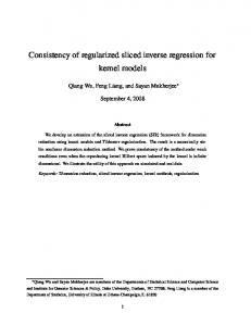
points from each category are used to plot the lowdimensional views to avoid excessive ink. The results are shown in Figure 1. Figures 1(a) and 1(b) are 2D views via PCA and SIR. There are some obvious overlaps among these ten classes. Figure 1(c) is the 2D view along KSIR directions and Figure 1(d) zooms in a small crowded region for a better view. We can easily see that KSIR variates provide a much better discriminant power. The next two examples are on regression data sets. The first one is the “peaks” function provided by Matlab. It creates a synthetic regression surface (without additive noise) using 2-dimensional inputs. The corresponding regression surface plot with 961 points is in Figure 2(a). In our study, we split this data set into 80% and 20% subsets for training and testing, respectively. Plots of 2D views by PCA, SIR and KSIR are in Figures 2(b)-(d). As the peaks data have only 2-dimensional inputs, there is not much sense to talk about dimension reduction in the 2D pattern space. The purpose of this data example is to show the relevant linear structure in feature subspace by KSIR as depicted in Figure 2(d). We can clearly see that the KSIR processing turns the nonlinear structure in pattern space into a prominent linear structure in kernel feature space. It provides an empirical justification to combine the KSIR with linear learning algorithms for other tasks on the feature e.d.r. subspace. Another regression example is the Friedman’s example (5). There are ten explanatory variables, but only five of them are effective and the rest are nuisance. There are linear component, 10x4 + 5x5 , as well as nonlinear component, sin(πx1 x2 ), and a hidden e.d.r. direction x3 to SIR in this example. We split the data into 99% and

JOURNAL OF LATEX CLASS FILES, VOL. 6, NO. 1, JANUARY 2007

PCA−2

0

−0.5

−1 −1

−0.5

0 PCA−1 (a)

0.5

1

−1 −1

1

−0.5

0 KSIR−1 (c)

KSIR−2

KSIR−2

0.5

−1 −1

0 SIR−1 (b)

0.5

−0.2

1 8

−0.4 1

8

1 33 3 33 3 3333 3 3

−0.8

1

1

1 9 9 9 9 9 5 999 99 9 9 5 5 59 5 5 555 5 5 5

−0.6 −0.4 KSIR−1 (d)

−0.2

Fig. 1. 2D views of pendigits data by PCA, SIR, KSIR.

Response (Y)

Response (Y)

5 0 −5 −10 5

0

−5 5 0

0 −5 −5

Variable−2

−10 −1

Variable−1

−0.5

0 PCA−1 (b)

0.5

1

−0.5

0 KSIR−1 (d)

0.5

1

10

5

5 Response (Y)

Response (Y)

(a) 10

0

−5

−10 −1

0

−5

−0.5

0 SIR−1 (c)

0.5

1

−10 −1

20 15 10

Response (Y)

25

Response (Y)

30

25 20 15 10 5 −0.5

0 PCA−1 (a)

0.5

1

0 −1

20 15 10 5

−0.5

0 SIR−1 (c)

0.5

1

0 −1

−0.5

0 KSIR−1 (c)

0.5

1

Fig. 3. 2D views of Friedman data by PCA, SIR and KSIR. are shown in Figure 3. Obviously, none of the PCA directions capture a good effective subspace for the response surface. The first SIR direction does reflect a good description for the response, and the first KSIR direction is even better and it carries the best information content for the response among the three methods. Figure 3(c) shows a clearly good linearity of the first KSIR variate to the response. In summary, the effect of KSIR is not mere dimension reduction, it also maps the data to lowdimensional nonlinear features via kernel transformation so that the response can be well approximated by a linear form in terms of these extracted nonlinear features. 4.2 KSIR dimension reduction for classification

10 10 5

30

25

0 −1

8 8 88 88 83 88

7 0.1 2 27 777 22 1772 7 7 2 2 222 2 2 2171171 0 71 1111 −0.1

−0.3 66 6 66 6 6 6 66 6 0.5

−0.5

30

5

8 8

0 0000 0 0000 000

8 88 888883 7777 22271 7 8 7 8 7 2 2 2 7 711 0 222211 8 71 1 11 11 1 3 333 33 31 9 5 9 33 3 999999 3 5999 64 5 9 5 5 555 5 5 55 44 44 44 44 −0.5 44 44 4 6

44 4 44 444 4 44 9 4 4 4 0.5 9 3 59 6 9 6 2 6 6 6 9 59 0 2 1 1155 99 60 660 2 222 1 7 2 6 9 566 0 00 0 2111 7 71 11 9995 2222211 1 7 7373 3 6 8 2 7 7 7 3 3 3 89 000 0 5 77 5 35 73 3333 7 5 5 88 0 8 0 0 5 6 8 0 −0.5 5 8 88 7 8 8 8

Response (Y)

0.5

1

9 3 9 0 9 99 000 00 9 999 9 5 0 00 0 4 6 4 6 4 0 999 64 666 535 4 4 6 4 4 444 5 533333355 08 73 33 66 4 8 8800 6 8 3 11 47 6 1 7 8 6 1 4 61 1 2 2 8 8 8 5 2 7 1 8 5 2 8 8 1 5 5 8 55 7 7 7 2 7 111 2 21 1 2 777 72 7 722 222

SIR−2

1

8

Fig. 2. 2D views of response vs. the 1st variate by PCA, SIR and KSIR with peaks data. 1% subsets for training and testing, respectively, for data visualization purpose. The leading ten eigenvalues by SIR and KSIR are respectively SIR : 0.7213, 0.0067, 0.0020, 0.0013, 0.0011, 0.0007, 0.0004, 0.0004, 0.0003, 0.0001; KSIR : 0.9417, 0.6639, 0.2010, 0.0435, 0.0214, 0.0120, 0.0111, 0.0105, 0.0097, 0.0092. The low-dimensional data views by PCA, SIR and KSIR

The dimension reduction provided by KSIR can be used as a data preprocess for later tasks such as classification or regression. In the process of applying SIR or KSIR, the role of each slice represents the clustering structure of the data. If we know the information about clustering structure in advance, it helps us to make slices when applying SIR or KSIR. In classification, the clustering structure has been defined through their class labels, and slices are made accordingly. We then estimate the central feature e.d.r. subspace and map the data onto this feature subspace for discriminant purpose. In a J-class problem, we slice the data sets into J slices according to the class labels. Thus, there are at most J − 1 many independent e.d.r. directions, since the rank of ΣE(A|YJ ) or ΣE(K|YJ ) is at most J − 1. After extracting the feature e.d.r. subspace, discriminant analysis becomes much computationally easier in this very low-dimensional subspace. Since we have turned the nonlinear structure in the pattern space into an approximately linear structure in the feature space via kernel transformation, direct application of linear learning algorithms on KSIR variates is often sufficient. In our classification experiments, we particularly pick the Fisher linear discriminant analysis (FDA) and the linear smooth support vector machine (SSVM) [23] as our baseline linear learning algorithms. One property of SSVM is that it is solved in the primal space and its computational complexity depends on the number of input attributes (here is the number of KSIR variates, which is at most J − 1). A smaller number of columns implies less computational load. Note that as data are projected along the KSIR directions, discriminant analysis is computationally light. The FDA and SSVM acting on top of KSIR variates are numerically compared with

JOURNAL OF LATEX CLASS FILES, VOL. 6, NO. 1, JANUARY 2007

the standard nonlinear SVM benchmark algorithm LIBSVM. For binary classification, the data sets put on experiments are already divided into training set and testing set in advance. We use the training set to build the model, including extracting the feature e.d.r. subspace and training for the final model in this e.d.r. subspace, then evaluate the resulting model using the testing set. As there is some stochastic variation due to reduced set selection, the procedure is repeated 10 times. We report the average error rate and the standard deviation of 10 times experiments. The upper panel of Table 3 lists the average error rates for these binary classifications. Reduced kernel approximation by a stratified random (training) subset is used depending on the data set size. The standard deviations reported in our numerical results are very small. It indicates that the reduced set sizes are large enough in our experiments from model robustness point of view. For binary classification, KSIR extracts a one-dimensional feature component for discriminant analysis. FDA in this one-dimensional subspace is a simple division of the line through the midpoint of two class centroids. The SSVM division of the line is a bit more complex than cutting through the midpoint. It is still a maximum margin criterion, but along a line instead of in a high-dimensional feature space. Results are compared with LIBSVM. Although FDA and SSVM are acting on top of a one-dimensional KSIR variate and reduced kernel approximation has been applied, the results in the KSIR columns are comparable to those in the LIBSVM column. It means that KSIR actually finds an effective projection direction in the kernel feature space and the reduced kernel approximation works well, too. For multi-class problems, the first four data sets are not pre-divided into training and testing sets. For these data sets, we use ten-fold cross validation and report their average error rates over 10 replicate runs of tenfold partition. Results are listed in the middle panel of Table 3. For the rest multi-class data sets, there are separate testing sets. The results of ten replicate runs are reported in the lower panel of Table 3. In these multiclass classification problems, one-versus-one scheme is used for SSVM and LIBSVM. Note that for the medline data set, the variable dimensionality is 22095. For this example we look for linear e.d.r. directions in the original pattern space instead of kernel e.d.r. directions. As the dimensionality is so high that a direct application of the classical SIR, which calls for covariance matrices of size 22095, is not possible. Our KSIR algorithm can overcome this problem by using the linear kernel, K = AA0 (even the reduced linear kernel, K = AA˜0 ). In linear kernel setting, the computation cost is at most O(n3 ), where n is the sample size. This is the special handling for data sets with n ¿ p, which is commonly seen in text mining and gene expression data sets. From Table 3, we see that a simple linear SSVM algorithm acting on a few leading KSIR variates can perform as good as LIBSVM. The performance of FDA on KSIR variates is a little

9

TABLE 3 The error rate for FDA and linear SSVM on KSIR variates compared with LIBSVM on classification data sets. Data set banana tree splice adult web Iris wine vehicle segment dna satimage pendigits medline

KSIR+FDA mean (std) 0.1176 (0.0039) 0.1225 (0.0027) 0.1182 (0.0041) 0.1702 (0.0011) 0.0164 (0.0007) 0.0227 (0.0064) 0.0163 (0.0053) 0.1460 (0.0091) 0.0297 (0.0025) 0.0652 (0.0035) 0.0926 (0.0031) 0.0229 (0.0011) 0.1208

KSIR+SSVM mean (std) 0.1183 (0.0028) 0.1156 (0.0023) 0.1175 (0.0036) 0.1492 (0.0008) 0.0152 (0.0004) 0.0273 (0.0066) 0.0125 (0.0042) 0.1499 (0.0103) 0.0282 (0.0020) 0.0447 (0.0013) 0.0914 (0.0034) 0.0193 (0.0027) 0.1136

LIBSVM mean (std) 0.1229 0.1283 0.1048 0.1491 0.0090 0.0373 (0.0034) 0.0187 (0.0042) 0.1460 (0.0072) 0.0285 (0.0016) 0.0463 0.0870 0.0180 0.1106

worse than SSVM on KSIR variates and LIBSVM, but the difference is small. Another issue is the computing time comparison. We record all the computing time CPU seconds in Table 4. All the experiments are executed in the same environment. The equipment of the computer is CPU P4 3.0GHz, Memory 1.5G and operating system XP. It can be seen that KSIR+FDA and KSIR+SSVM are often faster than LIBSVM in training time especially for large data sets and multi-class problems. For multi-class problems, we used “one-versus-one” scheme for SSVM and LIBSVM to decompose the problem into a series of binary classification subproblems and combine them by a majority vote. The KSIR+FDA and KSIR+SSVM only have to run the KSIR algorithm once, which consumes the major part of the computing time in one complete run of discriminant analysis. Once we have the e.d.r. variates with dimensionality J − 1, a series of binary SSVMs or one FDA machine in this (J −1)-dimensional subspace is computationally light to carry out. In comparing the hybrid of KSIR with linear ¡SSVM versus the LIBSVM, both ¢ have to build a series of J2 many binary classifiers. The former needs a one-time-only KSIR process in a reduced feature subspace of dimensionality n ˜ and then builds a series of binary classifiers in a (J − 1)-dimensional KSIR extracted subspace, while the latter builds such a series of binary classifiers in a higher dimensional feature space of dimensionality about the size 2n/J. We only report the training time comparison with LIBSVM. The testing time for linear learning algorithms (FDA and SSVM here, and RLS-SVR in next subsection) on KSIR test variates are prominently and uniformly faster than LIBSVM in regression and in classification, and thus we omit the report of testing time comparison. The efficient testing time is due to the fact that KSIR-based learning algorithms are acting on very low-dimensional KSIR variates, while LIBSVM is acting in the high dimensional feature space and its speed depends on the number of support vectors, which is much larger than the e.d.r. dimensionality.

JOURNAL OF LATEX CLASS FILES, VOL. 6, NO. 1, JANUARY 2007

10

TABLE 4 The training time (seconds) of FDA and linear SSVM on KSIR variates compared with LIBSVM on classification data sets.

4.3 KSIR dimension reduction for regression Different from classification problems, KSIR for regression can be more complicated than classification due to the lack of intuitive slices. In fact, we need to consider more factors, like the number of slices, their positioning and the dimensionality of the final e.d.r. subspace. For positioning of slices, we adopt a simple equal frequency strategy for it. For the number of slices, we run the experiments with various numbers of slices in the range of 15 to 45. We report the statistics such as mean, standard deviation and median, etc. of these experiments in Table 5. These results are quite robust to the number of slices.3 Similar conclusion for SIR can be found in [3]. Thus, we fix at 30 slices in the rest of regression examples. In determining the number of extracted components, there are formal statistical tests [3], [24], [25], [26], [27] for the linear case. Extension of these formal statistical tests to the kernel case has to be carefully studied and justified, which can be an interesting and important future direction. Here we present a bootstrapbased graphical tool which combines the variability plot [28] together with the scree plot [29] for further suggestion of the dimensionality d. The scree plot gives a pictorial view of the eigenvalues and how they drop. In our empirical experience, the last few eigenvalues are relatively much smaller than the leading ones. The variability plot further quantifies the variability, or the stability which is one minus the variability, for each eigen-component. The variability of the jth component is defined to be ρj =

B ´ 1 X³ (j) 1 − cos(θk ) , B k=1

(j)

where θk is the angle between the jth eigen-component and its bootstrapped estimate (repeated B times). Low variability indicates the corresponding eigenvector is stable and is regarded as a major component, while high variability indicates a minor component and can be regarded as noise. Here, we present the variability 3. For the CA_1000 and CA, the low R2 occurs at the slice number 15. By increasing the slice number, the low R2 phenomenon easily disappears.

0.8

0.8

eigenvalue

LIBSVM 0.041 0.075 0.443 219.3 149.5 2.806 3.654 2.402 3.032

Housing (scree plot) 1

0.6

0.4

0.2

0

0.6

0.4

0.2

0

0 2 4 6 8 10 12 14 16 18 20 22 24 26 ith component

0 2 4 6 8 10 12 14 16 18 20 22 24 26 ith component

Friedman (variability plot)

Friedman (scree plot)

1

1

0.8

0.8

eigenvalue

KSIR+SSVM 0.064 0.078 0.185 4.867 16.37 0.360 3.197 1.775 1.799

variability

KSIR+FDA 0.065 0.076 0.219 4.863 16.18 0.378 3.041 1.245 1.701

variability

Data set banana tree splice adult web dna satimage pendigits medline

Housing (variability plot) 1

0.6

0.4

0.2

0

0.6

0.4

0.2

0 2 4 6 8 10 12 14 16 18 20 22 24 26 ith component

0

0 2 4 6 8 10 12 14 16 18 20 22 24 26 ith component

Fig. 4. The variability plot and scree plot for Housing and Friedman data sets and scree plots for Housing and Friedman data sets (see Figure 4) with B = 50. These plots suggest using a small dimensionality. From this observation, we run the regression experiments on a small dimensionality (3 dimensions) as well as J − 1 dimensions. After extracting the KSIR directions, we apply the linear regularized least square (RLS) fit of the responses on KSIR variates. The testing results of KSIR+RLS are compared with nonlinear SVR provided in LIBSVM. Note that a reduced kernel approximation has been used in KSIR for all our regression examples. The R2 values based on ten-fold cross validation are shown in Table 6. R2 is a commonly used criterion for evaluation of regression goodness of fit. Its definition is given below: R2 = 1 −

n X i=1

(yi − yˆi )2 /

n X (yi − y¯)2 , i=1

where yˆi is the fitted response and y¯ is the grand mean. We can see that the difference in R2 between KSIR(29)+RLS and LIBSVM is not significant. Note that LIBSVM is only a little better than KSIR(3)+RLS. In other words, a small dimensionality, such as 3, can still achieve roughly the same performance as using the full dimensionality of 29 for 30 slices. Often a few leading directions, say 3, can be well enough for describing the response without losing much information. That fits the purpose if the data visualization is required. Computing time comparison is reported in Table 7. KSIR+RLS is much faster than LIBSVM, especially for large data problems. All these results reflect the same phenomenon found in classification, that KSIR can find effective feature e.d.r. directions to speed up the computation for regression fit with satisfactory results.

JOURNAL OF LATEX CLASS FILES, VOL. 6, NO. 1, JANUARY 2007

11

TABLE 5 R2 using 30 slices and statistics for R2 over 15-45 slices. Data set Housing Kf_1000 CA_1000 Kin_fh CA Friedman

R2 for 30 slices 0.8582 0.6480 0.9704 0.6955 0.9774 0.9555

mean 0.8584 0.6478 0.9553 0.6954 0.9719 0.9555

TABLE 6 R2 of RLS on 3 and 29 KSIR variates compared with LIBSVM on regression data sets. Data set Housing Kf_1000 CA_1000 Kin_fh CA Friedman

KSIR(3)+RLS mean (std) 0.8619 (0.0398) 0.6457 (0.0479) 0.9606 (0.0094) 0.6949 (0.0129) 0.9733 (0.0047) 0.9553 (0.0006)

KSIR(29)+RLS mean (std) 0.8611 (0.0440) 0.6473 (0.0462) 0.9702 (0.0055) 0.6950 (0.0128) 0.9770 (0.0031) 0.9554 (0.0006)

For multiresponse regression problems, we generate a synthetic data set modified from the Friedman example. 10 response variables and 10 predictor variables are generated as follows. The predictor variables x1 , . . . , x10 are independent and identically distributed uniformly over [0, 1], and the 10 response variables are generated from the following setting: 10 sin(πx1 x2 ) + 5(x3 − 0.5)2 + x4 + x5 + ², 10 sin(πx1 x2 ) + 20(x3 − 0.5)2 + 10x4 + 5x5 + ², 5y1 + ², y1 + y2 + ², y10 ∼ N (0, 0.1, ), N (0, 1).

A random sample of size 2000 is generated. Though the responses are in a 10-dimensional space, the effective dimensionality is actually only 2. Here are the steps for handling such a multiresponse regression using KSIR. •

•

Make kernel data (full or reduced) using predictor variables, denoted by K. Denote the observed multiresponses by Y . Compute correlation matrix of K and Y , denoted by Rcor , which is of size m × q, where m is the column size of K and q is the column size of Y . (One may use covariance matrix as well.) Extract the leading k right singular vectors (here k = 2 for the modified Friedman example) of Rcor and project Y onto these k leading directions, i.e., Rcor = U SV 0 (U and V are orthogonal matrices and S is diagonal) and let Y˜ = Y V˜ , where V˜ is the leading k columns of V .

min 0.8553 0.6462 0.8609 0.6948 0.9127 0.9554

TABLE 7 The training time (seconds) of RLS on 3 and 29 KSIR variates compared with LIBSVM on regression data sets.

LIBSVM mean (std) 0.8680 (0.0314) 0.6470 (0.0459) 0.9783 (0.0056) 0.7004 (0.0131) 0.9821 (0.0022) 0.9561 (0.0005)

4.4 KSIR dimension reduction for multiresponse regression

y1 = y2 = y3 = y4 = y5 . . . ² ∼

R2 over 15-45 slices std median max 0.0019 0.8580 0.8648 0.0008 0.6481 0.6490 0.0299 0.9699 0.9748 0.0003 0.6953 0.6960 0.0143 0.9776 0.9789 0.0001 0.9556 0.9556

Data set Housing Kf_1000 CA_1000 Kin_fh CA Friedman

•

•

•

KSIR(3)+RLS 0.021 0.015 0.016 1.029 0.167 6.064

KSIR(29)+RLS 0.035 0.024 0.042 1.121 0.376 6.433

LIBSVM 0.244 0.371 0.502 19.57 27.50 2242.1

Often k ¿ dim(Y ), and we call Y˜ the most correlated variates with K. Make slices using these lowdimensional most correlated variates (grid slicing along these Y˜ variates). In other words, we have J k slices for the data. Solve the generalized eigenvalue problem of between-slice covariance with respect to the kernel data covariance to extract KSIR variates. Perform regression of Y on KSIR variates for an allresponses regression, or perform regression of Y˜ on KSIR variates for only the most correlated response variates.

In our procedure, we use Cor(K, Y ) (or one could use Cov(K, Y ) alternatively) to look for the most correlated directions between K and Y . These leading most correlated variates are used to make slices, and then KSIR is carried out based on these slices. Next, regression is made on KSIR variates. To examine the performance of the KSIR applied to multiresponse regression, we run the regression of Y on KSIR variates using RLS and compare the results with a coordinate-wise nonlinear SVR using LIBSVM (one run for each response and there are 10 in total). Figure 5 displays the resulting R2 via the ten-fold cross validation for various numbers of slices. R2 for multiresponse regression is defined as

R2 = 1 −

q q n X n X X X (yij − yˆij )2 / (yij − y¯j )2 . i=1 j=1

i=1 j=1

The results evidence the good performance of KSIR based the most correlated response variates. Besides, the results from Figure 5 also reflect the robustness on the number of slices.

JOURNAL OF LATEX CLASS FILES, VOL. 6, NO. 1, JANUARY 2007

1 0.98

LIBSVM (coordinate−wise) KSIR−multiresponse rgreesion

0.96 0.94

R2

0.92 0.9 0.88 0.86

12

subspace, an optimal C is determined over a range of grid points. This tuning procedure at the second stage for C is computationally light, as it is carried out in a very low-dimensional e.d.r. subspace and the time complexity of linear SSVM and RLS depend on the dimensionality of the e.d.r. subspace. For each fixed γ we can try a few C values to pair with this γ without much computing cost. This is another computing merit of KSIR approach in practical usage. Note that all the parameters C and γ of each data set in our experiments are reported in Table 8 and 9.

0.84

5

0.82 0.8

4 5 6 7 8 9 10 11 12 13 14 15 16 17 18 19 20 21 Number of slices (square root)

Fig. 5. R2 for multiresponse modified Friedman example.

4.5 Kernels and parameter tuning In nonparametric statistics, the choice of kernel type is often not crucial as long as the chosen kernel constitutes suitable building blocks for the underlying functional class. There will be some slight difference in estimation efficiency for different choice of kernels. A list of kernels for nonparametric estimation and their relative efficiencies can be found in [30] (Table 3.1). Gaussian kernel K(x, u) = exp(−γkx − uk2 ) is probably the most commonly used kernel in SVM-based learning algorithms and we adopt it for the kernel extension of SIR in our nonlinear numerical examples. On the other hand, the choice of kernel bandwidth is much more crucial than the kernel type. For either KSIR-based methods or for the conventional SVMs, there are two parameters involved, namely, the weight parameter C and the Gaussian kernel width parameter γ. The naive tuning procedure, a two-dimensional grid search, is time consuming. A remedy for it is to replace the bulldozer grid-search by a well-designed search scheme to reduce computing load. For instance, the nested uniform design (UD) model selection method [31] provides an economic alternative for parameter tuning. It has been numerically shown that there is no significant difference in testing accuracy by using a nested-UD search to replace the grid search. Thus, in our experimental study, the nested-UD is adopted for parameter tuning in LIBSVM. As for KSIRbased methods, computing time for parameter tuning is a lot lighter than that for conventional SVMs, even if the latter is equipped with a UD-based search. Tuning procedure for KSIR-based methods is nearly a one-dimensional search for γ, as the search for C is computationally light and negligible. KSIR-based methods are carried out in two stages. At the first stage, a parameter value for γ is needed for training KSIR e.d.r. subspace. At the second, a parameter value for C is needed for linear SSVM or RLS on KSIR variates. For each γ and its resulting e.d.r.

C ONCLUSION

We have reformulated the KSIR [8] in a more rigorous and formal RKHS framework for theoretical development and for practical implementation of fast algorithm. The KSIR algorithm first maps the pattern space to an appropriate RKHS, and next extracts the main linear features in this embedded feature space. It takes class labels or regression response information into account and is a supervised dimension reduction method. After the extraction of the feature e.d.r. subspace, many supervised linear learning algorithms, such as FDA, SVM, SVR and possible others, can be applied to the images of input data in this feature e.d.r. subspace. This will generate a nonlinear learning model in the original input pattern space and achieve a very good performance for complex data analysis. We have also incorporated reduced kernel approximation to cut down the computational load and to resolve the numerical instability due to singularity in large between-slice covariance matrix. The singularity problem not only causes numerical instability but also leads to inferior e.d.r. directions estimation. A few leading components extracted by KSIR can carry most of the relevant information about y in regression and in classification. It allows us to run linear learning algorithms in a very low dimensional feature e.d.r. subspace and to gain computational advantages without sacrificing the performance of learning algorithms. For example in solving ¡ ¢nonlinear SVM multi-class problem, one has to solve J2 nonlinear binary SVMs under the “one-versus-one” scheme. In KSIR-based approach, it only involves solving the KSIR problem ¡ ¢once, and the remaining task is solved by a series of J2 many linear binary SVMs in a (J − 1)-dimensional space. Moreover, KSIR approach also has an advantage in tuning procedure. We have demonstrated these nice merits in our numerical experiments. Finally, using the first one or two components will help scientists or data analysts to gain a direct insight of data patterns, which will be otherwise complex in high dimensionality.

A PPENDIX A KSIR IN AN RKHS F RAMEWORK The classical SIR looks for e.d.r. directions in the pattern Euclidean space for maximum between-slice dispersion

JOURNAL OF LATEX CLASS FILES, VOL. 6, NO. 1, JANUARY 2007

13

TABLE 8 The parameters C and γ in each classification data set Data set banana tree splice adult web Iris wine vehicle segment dna satimage pendigits medline

KSIR+FDA γ 8 5.00 × 10−1 3.91 × 10−3 4.88 × 10−4 5.00 × 10−1 6.25 × 10−2 6.25 × 10−2 3.10 × 10−2 2.50 × 10−1 9.76 × 10−4 5.00 × 10−1 6.25 × 10−2 -

KSIR+SSVM C γ 3.16 × 104 5.76 1.00 × 103 1.34 × 10−1 1.78 × 105 1.61 × 10−3 5.62 × 103 4.49 × 10−4 1.00 × 103 1.40 × 10−1 1.00 × 103 1.98 × 10−1 1.00 × 101 1.94 × 10−2 3.16 × 104 3.10 × 10−2 5.62 4.78 × 10−1 5.62 × 103 2.53 × 10−4 5.62 3.20 × 10−1 5.62 1.61 × 10−1 1.00 × 10−1 -

LIBSVM C γ 1.00 × 102 4.19 1 9.31 × 10−1 1.00 × 102 2.89 × 10−2 1.00 × 101 1.98 × 10−2 1.00 × 101 3.76 × 10−2 4.09 × 103 1.95 × 10−3 1.28 × 102 9.76 × 10−4 5.12 × 102 1.25 × 10−1 6.4 × 101 1 1.00 × 102 2.53 × 10−2 1.60 × 101 1 1.00 × 101 4.65 × 10−1 1.00 × 101 -

TABLE 9 The parameters C and γ in each regression data set Data set Housing Kf_1000 CA_1000 Kin_fh CA Friedman

KSIR(3)+RLS C γ 1.00 × 106 4.15 × 10−1 1.78 × 105 5.06 × 10−4 1.00 × 103 2.00 × 10−3 3.16 × 101 9.90 × 10−3 1.79 × 102 2.80 × 10−3 1.00 × 103 9.11 × 10−2

KSIR(29)+RLS C γ 1.00 × 106 4.15 × 10−1 5.62 × 103 5.06 × 10−4 1.78 × 102 2.00 × 10−3 1 9.90 × 10−3 1.79 × 102 2.80 × 10−3 1.00 × 103 9.11 × 10−2

LIBSVM C γ 1.00 × 102 4.11 × 10−1 1 2.53 × 10−2 3.16 × 102 1.15 × 10−1 1 2.66 × 10−2 1.00 × 102 1.15 1.00 × 102 1.83 × 10−1

with respect to overall dispersion. Based on the same idea of maximum between-slice dispersion, the kernel transform embeds the Euclidean pattern space X into an appropriate HK by Γ : x 7→ K(x, ·). Next KSIR looks for e.d.r. directions in HK that maximizes the betweenslice dispersion with respect to the total dispersion. For technical details, we need to introduce a few more notations. Define below the grand mean function m(·), conditional mean function my (·), covariance kernel Σ and between-slice covariance kernel ΣB :

Theorem 1* Assume the existence of a feature e.d.r. subspace H = span{h1 , . . . , hd } in HK and the validity of the LDC (10). Further assume that the covariance operator Σ is compact and non-singular and that my − m is in the range of Σ1/2 . 4 Then the central inverse regression curve my − m falls into the subspace Σ(H). Proof of Theorem 1*: Note that for any f, g ∈ HK we have hm, f iHK = EhK(x, ·), f (·)iHK = Ef (x) and hΣf, giHK = Cov{f (x), g(x)}. In particular, take g = K(u, ·) and f = hk , we have

m(s) = E{K(x, s)}, my (s) = E {K(x, s)|y} , Σ(s, t) = E {(K(x, s) − m(s))(K(x, t) − m(t))} , ΣB (s, t) = E {(my (s) − m(s))(my (t) − m(t))} .

hΣhk , giHK = Cov{hk (x), K(x, u)}.

(20) (21) (22) (23)

Σ and ΣB are also called covariance operators, as they Rinduce linear operators on HK given by (Σf )(·) = K(x, ·)f (x)dPx (x) and Z (ΣB f )(·) = E (K(x, ·)|y) E (f (x)|y) dPy (y). KSIR solves the spectral decomposition of the betweenslice covariance operator ΣB with respect to the overall covariance operator Σ. That is, it aims to find leading directions hk ∈ HK to max ΣB hk = λk Σhk s.t. hhk , Σhk iHK = δkj ,

(24)

where δkk = 1 and δkj = 0 for k 6= j. Below is a functional version of Theorem 1.

(25)

Also the covariance of hi (x) and hj (x) is given by Cov{hi (x), hj (x)} = hΣhi , hj iHK .

(26)

Let ΣH denote the matrix with the (i, j)th entry given by (26) and let H(x) be the random vector (column vector) given by H(x) = (h1 (x), . . . , hd (x))0 . Note that ¯ ¾ ½ ¯ my (·) − m(·) = E E(K(x, ·)|H(x)) − m(·)¯¯y . By the LDC we have E(K(x, ·)|H(x)) − m(·) is linear in H(x), which leads to E(K(x, u)|H(x)) − m(u) = c(u)H(x), where c(u) = Cov{K(x, u), H(x)0 }Σ−1 H (a drow vector) by the application of least squares linear regression. From (25) we have 0 −1 c(u) = hΣH(·)0 , K(·, u)iHK Σ−1 H = (ΣH(u)) ΣH .

4. The compactness condition is to ensure that hf, ΣgiHK is welldefined and the last condition on my − m is to ensure that hmy − m, Σ−1 (my − m)iHK exists and won’t go unbounded.

JOURNAL OF LATEX CLASS FILES, VOL. 6, NO. 1, JANUARY 2007

ΣH(u) is independent of y and is in the linear span of {Σh1 (u), . . . , ΣK hd (u)}. ¤ Theorem 1* says that (my − m) falls into the subspace Σ(H). In other words, Σ−1 (my − m) is in the feature e.d.r. subspace. Thus, orthonormalized Σ−1 (my − m) can be used for the estimation of e.d.r. directions. The idea is first to slice the y-variable into J slices and denote the slice means by mj , i.e., mj (·) = E{K(x, ·)|y ∈ jth slice}. Next is to orthonormalize Σ−1 (mj − m), j = 1, . . . , J, and use them for feature e.d.r. directions. The idea can be formalized in the following proposition. Let M be a J × J matrix with (j, j 0 )th entry given by ¤ £√ πj πj 0 hmj − m, Σ−1 (mj 0 − m)iHK jj 0 , M := where πj is the prior probability for the jth slice. Denote its decomposition by M = U DU 0 , where U consists of eigenvectors with non-zero eigenvalues and D is a diagonal matrix of non-zero eigenvalues. Let W = (w1 , . . . , wJ ), J many functions arranged in row, where √ wj (u) = πj (mj (u)−m(u)) is the jth centered weighted slice mean. Proposition 2* Σ−1 W U D−1/2 are e.d.r. directions. Proof of Proposition 2*: To show this proposition, we have to check that there exists a certain positive definite diagonal matrix Λ such that ΣB (Σ−1 W U D−1/2 ) = Σ(Σ−1 W U D−1/2 )Λ and (Σ−1 W U D−1/2 )0 Σ (Σ−1 W U D−1/2 ) = I hold. Note that ΣB can be written as ΣB = W W 0 . Then, ΣB (Σ−1 W U D−1/2 ) = W W 0 Σ−1 W U D−1/2 = W U D1/2 .

14

[4] [5] [6] [7] [8] [9] [10] [11] [12]

[13] [14] [15] [16] [17] [18] [19] [20]

That is, take Λ = D. The derivation of the second assertion straightforwardly goes as follows:

[21]

D−1/2 U 0 W 0 Σ−1 W U D−1/2 = D−1/2 U 0 M U D−1/2 = I.

[22]

The proof is completed. ¤ In summary, KSIR is derived based on the same notion as SIR but in an infinite-dimensional RKHS. Its procedure is simply the SIR procedure on kernel transformed data.

[23] [24]

ACKNOWLEDGMENT

[26]

The authors thank Dr. Wu, Han-Ming for helpful discussion and thank four anonymous reviewers for many constructive comments. Special thanks go to an anonymous reviewer who has simplified our original proof for Proposition 2.

[25]

[27] [28] [29]

R EFERENCES [1] [2] [3]

E. Alpaydm, Introduction to Machine Learning. The MIT Press, 2004. R. D. Cook, Regression Graphics: Ideas for Studying Regressions Through Graphics. John Wiley and Sons, 1998. K. C. Li, “Sliced inverse regression for dimension reduction (with discussion),” Journal of the American Statistical Association, vol. 86, pp. 316–342, 1991.

[30] [31]

C. Chen and K. C. Li, “Can SIR be as popular as multiple linear regression?” Statistica Sinica, vol. 8, pp. 289–316, 1998. N. Duan and K. C. Li, “Slicing regression: a link free regression method,” Annals of Statistics, vol. 19, pp. 505–530, 1991. P. Hall and K. C. Li, “On almost linearity of low dimensional projection from high dimensional data,” Annals of Statistics, vol. 21, pp. 867–889, 1993. K. C. Li, “Nonlinear confounding in high-dimensional regression,” Annals of Statistics, vol. 25, pp. 577–612, 1997. H. M. Wu, “Kernel sliced inverse regression with applications on classification,” Journal of Computational and Graphical Statistics, vol. 17, no. 3, pp. 590–610, 2008. C. C. Chang and C. J. Lin., “LIBSVM: a library for support vector machines. Software available at http://www.csie.ntu.edu.tw/∼cjlin/libsvm,” 2001. J. H. Friedman, “Multivariate adaptative regression splines,” Annals of Statistics, vol. 19, pp. 1–67, 1991. G. Wahba, Spline Models for Observational Data. SIAM, 1990. G. Wahba, “Support vector machines, reproducing kernel Hillbert ¨ spaces, and randomized GACV,” In B. Scholkopf, C. J. C. Burges, and A. J. Smola, editors, Advances in Kernel Methods - Support Vector Learning. The MIT Press, 1999. S. Saitoh, Integral Transforms, Reproducing Kernels and Their Applications. Addison Wesley Longman, 1997. J. R. Thompson and R. A. Tapia, Nonparametric Function Estimation, Modeling, and Simulation. SIAM, 1990. P. Diaconis and D. Freedman, “Asymptotics of graphical projection pursuit,” Annals of Statistics, vol. 12, pp. 793–815, 1984. F. R. Bach and M. I. Jordan, “Kernel independent component analysis,” Journal of Machine Learning Research, vol. 3, pp. 1–48, 2002. Y. J. Lee and S. Y. Huang, “Reduced support vector machines: a statistical theory,” IEEE Transactions on Neural Networks, vol. 18, pp. 1–13, 2007. Y. J. Lee, H. Y. Lo, and S. Y. Huang, “Incremental reduced support vector machines,” International Conference on Informatics Cybernetics and System (ICICS2003), 2003. ¨ ¨ S. Mika, G. R¨atsch, J. Weston, and B. Scholkpf and K.-R. Muller, “Fisher discriminant analysis with kernels,” in Neural Networks for Signal Processing IX, 1999, pp. 41–48. J. C. Platt, “Sequential minimal optimization: a fast algorithm ¨ for training support vector machines,” In B. Scholkopf, C. J. C. Burges, and A. J. Smola, editors, Advances in Kernel Methods Support Vector Learning. The MIT Press, 1999. A. Asuncion and D. J. Newman, “UCI repository of machine learning databases. http://www.ics.uci.edu/∼mlearn/mlrepository.html,” 2007. MATLAB, User’s Guide. The MathWorks, Inc., Natick, MA 01760, 1992. Y. J. Lee and O. L. Mangasarian, “SSVM: A smooth support vector machine,” Computational Optimization and Applications, vol. 20, pp. 5–22, 2001. L. Ferr´e, “Determining the dimension in sliced inverse regression and related methods,” Journal of the American Statistical Association, vol. 93, pp. 132–140, 1998. J. R. Schott, “Determining the dimensionality in sliced inverse regression,” Journal of the American Statistical Association, vol. 89, pp. 141–148, 1994. S. Velilla, “Assessing the number of linear components in a general regression problem,” Journal of the American Statistical Association, vol. 93, pp. 1088–1098, 1998. Z. Ye and R. E. Weiss, “Using the bootstrap to select one of a new class of dimension reduction methods,” Journal of the American Statistical Association, vol. 98, pp. 968–979, 1998. I. P. Tu, H. Chen, H. P. Wu, and X. Chen, “An eigenvector variability plot,” Statistica Sinica, to appear. R. B. Cattell, “The scree test for the number of factors,” Multivariate Behavioral Research, vol. 1, pp. 245–76, 1966. B. W. Silverman, Density Estimation for Statistics and Data Analysis. Chapman and Hall, 1986. C. M. Huang, Y. J. Lee, D. K. J. Lin, and S. Y. Huang, “Model selection for support vector machines via uniform design,” A special issue on Machine Learning and Robust Data Mining of Computational Statistics and Data Analysis, vol. 52, pp. 335–346, 2007.

JOURNAL OF LATEX CLASS FILES, VOL. 6, NO. 1, JANUARY 2007

Yi-Ren Yeh received the M.S. degree from the Department of Computer Science and Information Engineering, National Taiwan University of Science and Technology, Taiwan in 2006. He is currently working toward the PhD degree in the Department of Computer Science and Information Engineering, National Taiwan University of Science and Technology. His research interests include machine learning, data mining, and information security.

Su-Yun Huang received the B.S. and M.S. degrees from Department of Mathematics, National Taiwan University, in 1983 and 1985, respectively, and the Ph.D. degree from Department of Statistics, Purdue University in 1990. She is currently a Research Fellow in the Institute of Statistical Science, Academia Sinica, Taiwan. Her research interests include mathematical statistics and statistical learning theory.

15

Yuh-Jye Lee received his Master degree in Applied Mathematics from the National Tsing Hua University, Taiwan in 1992 and PhD degree in computer sciences from the University of Wisconsin-Madison in 2001. He is an associate professor in the Dept. of Computer Science and Information Engineering, National Taiwan University of Science and Technology. His research interests are in machine learning, data mining, optimization, information security and operations research. Dr. Lee developed new algorithms for large data mining problems such as classification and regression problem, abnormal detection and dimension reduction. Using the methodologies such as support vector machines, reduced kernel method, chunking and smoothing techniques allow us to get a very robust solution (prediction) for a large dataset. These methods have been applied to solve many real world problems such as intrusion detection system (IDS), face detection, microarray gene expression analysis and breast cancer diagnosis and prognosis.