Consistent Covariance Matrix Estimation with

Consistent Covariance Matrix Estimation with Spatially Dependent Panel Data Author(s): John C. Driscoll and Aart C. Kraay Source: The Review of Economics and Statistics, Vol. 80, No. 4, (Nov., 1998), pp. 549-560 Published by: The MIT Press Stable URL: http://www.jstor.org/stable/2646837 Accessed: 03/06/2008 13:17 Your use of the JSTOR archive indicates your acceptance of JSTOR's Terms and Conditions of Use, available at http://www.jstor.org/page/info/about/policies/terms.jsp. JSTOR's Terms and Conditions of Use provides, in part, that unless you have obtained prior permission, you may not download an entire issue of a journal or multiple copies of articles, and you may use content in the JSTOR archive only for your personal, non-commercial use. Please contact the publisher regarding any further use of this work. Publisher contact information may be obtained at http://www.jstor.org/action/showPublisher?publisherCode=mitpress. Each copy of any part of a JSTOR transmission must contain the same copyright notice that appears on the screen or printed page of such transmission.

JSTOR is a not-for-profit organization founded in 1995 to build trusted digital archives for scholarship. We enable the scholarly community to preserve their work and the materials they rely upon, and to build a common research platform that promotes the discovery and use of these resources. For more information about JSTOR, please contact [email protected].

http://www.jstor.org

CONSISTENT COVARIANCE MATRIX ESTIMATION WITH SPATIALLY DEPENDENT PANEL DATA John C. Driscoll andAart C. Kraay* Abstract-Many paneldatasets encounteredin macroeconomics,international economics, regional science, and finance are characterizedby cross-sectionalor "spatial"dependence.Standardtechniquesthatfail to accountforthisdependencewill resultin inconsistentlyestimatedstandard elrors.In thispaperwe presentconditionsunderwhicha simpleextension of commonnonparametric covariancematrixestimationtechniquesyields standarderrorestimatesthatarerobustto verygeneralformsof spatialand temporaldependenceas the time dimensionbecomeslarge.We illustrate the relevance of this approachusing Monte Carlo simulationsand a numberof empiricalexamples.

dures are in general unknown. In view of this, it would appear to be desirable to implement nonparametric corrections for spatial dependence that are analogous to the standard nonparametric time-series corrections for serial dependence. However, this approach has two major drawbacks. First, in most applications there is no naturalordering in the cross-sectional dimension upon which to base the cross-sectional analogues of the necessary mixing conditions.2 Second, even if such an ordering were available, I. Introduction mixing conditions that require the dependence between two CROSS-SECTIONAL or "spatial"dependenceis a prob- observations that are "far apart" in the cross-sectional \ lematic aspect of many panel data sets in which the ordering to be small rule out canonical forms of crosscross-sectional units are not randomly sampled. For ex- sectional dependence such as equal cross-sectional correlaample, spatial correlations may be present in macroeconom- tions. In many applications, however, the time dimension of the ics, regional science, or international economics applicais sufficiently large to justify reliance on asymptotics panel tions in which the cross-sectional units are a nonrandom as T oo, holding fixed the size of the cross-sectional of or sample states, countries, industries observed over time, as these units are likely to be subject to both observable and dimension N. In this case, the problem of consistent unobservable common disturbances. Similarly, in finance covariance matrix estimation appears to be more tractable, applications, cross-sectional units may be shares or portfo- as it is in principle possible to obtain consistent estimates of lios of assets that respond, perhaps heterogeneously, to the N X N matrix of cross-sectional correlations by averagaggregate market shocks. Although this spatial dependence ing over the time dimension. The estimated cross-sectional generally will not interferewith consistent parameterestima- covariance matrix can then be used to construct standard tion, standardtechniques that fail to account for the presence errorswhich are robust to the presence of spatial correlation. of spatial correlations will yield inconsistent estimates of the The cross-sectional covariance matrix can be estimated either using parametric methods or using standard spectral standarderrors of these parameters. Corrections for spatial correlation are possible, but suffer density matrix estimation techniques of the sort popularized from a number of limitations. Consider first standardpanel in econometrics applications by Newey and West (1987). data techniques which assume a fixed time dimension of size Unfortunately this approach also has two drawbacks. First, T and require the cross-sectional dimension N to become in finite samples in which the cross-sectional dimension N is large for their asymptotic justification. In this case, paramet- large, these techniques may not be feasible since it will not ric corrections for spatial correlation are possible only if one be possible to obtain a nonsingular estimate of the N X N places strong restrictions on their form, since the number of matrix of cross-sectional correlations using the NT available spatial correlations increases at the rate N2, while the observations. Second, even when T is sufficiently large number of observations grows at only rate N.1 If the relative to N for the estimator to be feasible, its finite sample restrictions are misspecified, the properties of these proce- properties may be quite poor in situations where N and T are -

Received for publication March 13, 1997. Revision accepted for publication November 7, 1997. * Brown University; and The World Bank, respectively. We would like to thank John Campbell, Greg Mankiw, Matt Shapiro, and especially Gary Chamberlain and Jim Stock for helpful comments and suggestions, as well as several anonymous referees. Financial support from the Earle A. Chiles Foundation (Driscoll) and the Social Sciences and Humanities Research Council of Canada (Kraay) during work on earlier versions of this paper is gratefully acknowledged. An earlier version of this paper was circulated under the title "Spatial Correlations in Panel Data." The findings, interpretations, and conclusions expressed in this paper are entirely those of the authors.They do not necessarily represent the views of the World Bank, its Executive Directors, or the countries they represent. 1 A simple and common strategy is to assume that the spatial correlations are equal for every pair of cross-sectional units so that the inclusion of time dummies eliminates the spatial dependence. Keane and Runkle (1990), Case (1991), and Elliot (1993) are examples of more complicated parametric structures. Anselin (1988) provides a survey of the extensive regional science literature on this problem primarily in the context of pure

cross-sectionalregressions.Frees (1995) providesa discussionof testing for spatialcorrelationusinglarge-Nasymptotics. 2 Conley(1994) circumvents this difficultyby assumingthe existenceof priorinformationon a measureof distancein the cross-sectionaldimension. The paperof Froot(1989) representsan interestingcombinationof the parametricandnonparametric approaches.He imposesthe parametric restrictionthatsubgroups(industries)in the cross-sectionaldimensionof firmsareindependent,andthenappliesa panelanalogof theWhite(1980) covariancematrixestimationtechniquesto heteroskedasticity-consistent nonparametrically estimatethe sum of the diagonalblocks in the covariancematrix,relyingon large-Nasymptotics. 3 An exampleof the firstapproach is a variantof the seeminglyunrelated regressions(SUR) model of Zellner (1962) in which coefficients are restrictedto be equalacrossequations;three-stageleast squares(3SLS)in which a similarrestrictionis made is anotherexample.Variantson the second approachhave found some applicationin the financeliterature. Lehmann(1990) appliesthe Newey andWest(1987) techniquein a study of residualrisk, but does not provideconditionson the structureof the spatialcorrelationsunderwhichthis estimatoris consistent.

? 1998 by the Presidentand Fellows of HarvardCollege and the MassachusettsInstituteof Technology

[ 549 ]

550

THE REVIEW OF ECONOMICSAND STATISTICS

of comparable orders of magnitude, since the many elements of the cross-sectional covariance matrix will be poorly estimated. In this paper we propose a simple modification of the standardnonparametrictime series covariance matrix estimator which remedies the deficiencies of techniques which rely on large T asymptotics. In particular,we show that a simple transformation of the orthogonality conditions which identify the parameters of the model permits us to construct a covariance matrix estimator which is robust to very general forms of spatial and temporal dependence as the time dimension becomes large. The consistency result holds for any value of N, including the limiting case in which N ? ? at any rate relative to T. By relying on nonparametric techniques, we avoid the difficulties associated with misspecified parametricestimators. Moreover, since we do not place any restrictions on the limiting behavior of N, the size of the cross-sectional dimension in finite samples is no longer a constraint on feasibility, and we can be confident of the quality of the asymptotic approximation in finite samples in which N and T are of comparable size, or even if N is much larger than T, provided that T is sufficiently large. The remainder of this paper proceeds as follows. In section II we discuss the intuitions behind our approach, and then use mixing random fields to characterize a broad class of spatial and temporal dependence to which our covariance matrix estimator is robust. We then formally present the consistency result, which is a very simple variant on standard heteroskedasticity and autocorrelation consistent covariance matrix estimation techniques such as those in Newey and West (1987) or Andrews (1991). The next two sections emphasize the practical implications of spatial dependence for consistent covariance matrix estimation. Section III provides Monte Carlo simulations that demonstrate the consequences of failure to correct for spatial dependence, and compare the small-sample properties of the spatial correlation consistent estimator proposed here with common alternatives. We find that the presence of even modest spatial dependence can impart large biases to ordinary least squares (OLS) standard errors when the size of the cross-sectional dimension is large. We also show that the finite-sample performance of the spatial correlationconsistent estimator is very similar to that of the standard Newey and West (1987) time-series estimator, regardless of the size of the cross-sectional dimension. Moreover, despite the fact that the spatial correlation consistent standarderror estimator relies on large-T asymptotics, its finite-sample performance dominates that of common alternatives which do not take spatial dependence into account, even when the time dimension is quite short. Section IV presents three empirical examples in which correcting for spatial correlation yields estimated standarderrors that differ substantially from conventional estimates. Section V concludes.

II.

Consistent Covariance Matrix Estimation with Spatial Dependence

A. Intuitions In order to fix ideas, consider the class of models combining cross-sectional and time series data that is identified by an R X 1 vector of orthogonality conditions E[hi,(O)] = 0, where hit(O)= h(zit,0), zi, is a vector of data, 0 is a K X 1 vector of parameterswith K < R, and the time and unit subscripts vary over t = 1, . . ., T and i = 1, ... , N. Under the assumption that N is fixed, conventional timeseries generalized method of moments (GMM) estimation of these models proceeds by stacking the R orthogonality conditions for each of the N observations to obtain an NR X 1 vector of moment conditions E[ht(O)] = 0, where ht(0) = [hlt(O)'g... , hNt (0)']'. Provided that ht(0) satisfies wellknown regularity conditions,4 it is straightforwardto construct the GMM estimator of the parametervector 0 as h0)] t

OT= argmin

ST

fht(0)]

where STis a consistent estimator of the NR X NR matrix, -

ST=,

T

iT -

:

:7 t=1 s=l

t

E[h,(O)hs(0)']

It is well known that consistent estimation of the variance of the GMM estimator also requires a consistent estimate of this matrix, and Newey and West (1987) have shown that a positive semidefinite estimator of ST can be obtained using spectral density matrix estimation techniques. In many data sets encountered in macroeconomics, international economics, or finance, the size of the crosssectional dimension N may be very large relative to the time dimension T. For example, tests of purchasing power parity or of consumption risk sharing are commonly carried out with samples of more than 100 countries, using 20 or 30 annual observations. In such situations, two difficulties arise. First, if the size of the cross-sectional dimension is too large relative to the time series dimension, it will not be possible to estimate the NR(NR + 1)/2 distinct elements in the matrix ST using the NT available observations in a manner which yields a nonsingular estimate. In this case, it is necessary to place prior restrictions on the form of the spatial correlations in order to reduce the dimensionality of the problem. Second, even if these estimators are feasible, the quality of the asymptotic approximation that is used to justify them is suspect, as the asymptotic theory implies that the ratio NIT 4 For example, standard results on the consistency and asymptotic normality of the GMM estimator require that hk(O)be an NR-dimensional mixing sequence with bounded (4 + 8)th moments, and a measurable and continuously differentiable function of 0.

COVARIANCEMATRIXESTIMATIONWITH SPATIALLYDEPENDENT PANEL DATA tends to zero while in the finite sample N is in fact much larger than T. In light of these two difficulties, it would be desirable to have an estimator which will be feasible even when N is large relative to T, and which does not require the assumption that N is constant for its asymptotic justification. We achieve this by basing our estimation on the following simple transformationof the orthogonality conditions. If we define an R X 1 vector of cross-sectional averages, h,(O) = (1/N) IN I hit(O), we can identify the model using only the R X 1 vector of cross-sectional averages of the moment conditions, that is, E[h,(O)] = 0. In this case, consistent estimation of the variance of the GMM estimator requires a consistent estimator of the R X R matrix,

ST =

i -

T'

T

T t=1 s=1

E[hh(O)hs(O)'].

Since ST has only R(R + 1)/2 distinct elements, the size of the cross-sectional dimension is no longer a constrainton the feasibility of estimating this matrix, eliminating the first difficulty.5 Moreover, since h,(O) is the sum of N elements normalized by N, it will have well-behaved moments for any value of N. This will allow us to make N any nondecreasing function of T in the proof of consistency of the usual covariance matrix estimator, hence addressing the second concern. A specific example may help to clarify our approach. Consider a simple univariate linear model with crosssectional but no time-series dependence, that is, Yit= xi43 + Eit with E[Eit] = 0 and E[xitEitxjtEjt]= ij for all i, j, and t, and which is identified by the assumption that E[XitEit]= 0. It is straightforwardto see that the GMM estimator of ,Bbased on the cross-sectional average of the orthogonality conditions, E[ht(Q)] = (1/N) I E [xit(yit - xit)] = 0 is simply the OLS estimator applied to the pooled time-series crosssectional data. Consistent estimation of the variance of this estimator requires a consistent estimate of the sum 1 T1 N1 N ST=

-

z

T t=1 j=1 =

N1 N1 E[xitXjtEitEjt] =

1=1 j=1

Oij

which can readily be constructed by replacing the unobserved disturbances with the estimated residuals.6 In contrast, suppose that we were to base our estimates on the N X 1 vector of orthogonality conditions, E[ht(Q)] = 0, where the ith element of ht(Q)is hit(t) = xit(yit - x it3). Consistent 5We are assumingthatthe numberof orthogonalityconditionsR is less than the numberof cross-sectionalunits N. This rules out applications wheretheparametersarepermittedto varyacrosscross-sectionalunits. 6 Clearly,OLSstandard errorsandheteroskedasticity-consistent standard errorswould resultin inconsistentestimatessince they are based on the assumptionthat the off-diagonalelements of the variance-covariance matrixof theerrorsarezero,thatis, wij= 0 for i 0 j.

551

estimation of the variance of this estimator requires a consistent estimate of the N X N matrix ST, whose ijth = wij. Since this element is 5Tij = (l/T)>2[I E[Xi,Xj,Ei,Ej,] procedure (which is the Zellner (1962) seemingly unrelated regressions (SUR) model with the slope coefficients constrained to be equal for each cross section) requires an estimate of each of the N(N + 1)/2 distinct elements in ST ratherthan simply an estimate of the sum of these elements, it clearly will not be feasible in situations where the cross-sectional dimension is large relative to the time series. Even when it is feasible, it is reasonable to expect that the finite sample performance of this estimator may be quite poor since each of the cross-sectional covariances will be poorly estimated unless the size of the cross-sectional dimension is small relative to the length of the time series dimension. In the following subsection, we formalize the intuitions presented here. First, we use mixing random fields to characterize a general class of spatial and temporal dependence for the random variables hit(O).Once we verify that the sequence of cross-sectional averages of these random variables satisfies the well-known conditions for consistent covariance matrix estimation (such as those in Newey and West (1987)), the consistency of the usual estimator of ST is immediate. B. RandomFields Random fields, which are simply collections of doublyindexed random variables, provide a natural framework for describing situations in which both the cross-sectional dimension as well as the time-series dimension of a data set are large.7 More formally, let Z2 denote the two-dimensional lattice of integers, Z2 = {(i, t) i = 1, 2, . . . N ... ., t = 1, 2,.. ., T, .. .1, and let (fQ, P) denote the standard probability triple. A random field is defined as follows: Definition: The set of random variables (f, g P) is a random field.

fEz z EEZ2

on

In order to summarize the cross-sectional and time-series dependence between the elements of the random field, consider sets of the form A, = {(i, v) v ' tl. The o-algebra generated by the collection of random variables whose indices lie in the set At, which we denote by YtQ Or(E Iz E At), has the usual interpretationas the information set available at time t. Furthermore, let 7 O-(E6zlz EE Atcs)9 where Ac denotes the complement of At. Using this notation, we can summarize the dependence between two or-algebrasusing o-mixing coefficients defined in a manner 7 Randomfield structureshave been used extensivelyin the statistics literature.See Rosenblatt(1970) and Bulinskii (1988) for asymptotic results.Doukhan(1994)providesan extensivesurveyof mixingin random fields in othercontexts.Some economicapplicationsincludeWooldridge andWhite(1988), Quah(1990, 1994),andConley(1994).


552

analogous to the standard univariate cx-mixing8coefficient, that is, ct(s)

sup

P [F1 n F2]P

sup

(FtCz,7-t_x,F2Cz,,t+s

Result 1: Suppose that hit(O), t = 1, . . . , T, i = 1, . .. , N(T), is an o-mixing random field of size r/(r - 1), r > 1. Then

[F1]P [F2]

)

We define a mixing random field as follows: A random field is cx-mixing of size r/(r r > 1, if for some X > r/(r - 1), cx(s) = 0(s-X). Definition:

-

1),

This definition of mixing departs from the more standard cx-mixing structures on random fields in that it treats the cross-sectional dependence differently than the time-series dependence. Most definitions of mixing restrict the dependence in both dimensions symmetrically, requiring the dependence between two observations to decline either as the distance in the cross-sectional orderingbecomes large, or as the time separation becomes large. This restriction on the dependence across units is required to deliver (NT) 1/2 asymptotic normality for double sums over i and t of the Eit, just as in the one-dimensional case restrictions on the temporal dependence are required to deliver T1/2 asymptotic normality for appropriatelynormalized sums.9 The definition of mixing presented here, however, does not restrict the degree of cross-sectional dependence. Instead, we only require the dependence between Eit and Ejt-s to be small when s is large, for any value of i and j. The advantage of this is that it will not preclude canonical forms of cross-sectional dependence, such as factor structures in which cross-sectional units may be equicorrelatedin a given time period, or grouped structuresin which observations are correlated according to possibly unobservable group characteristics. This greater permissible cross-sectional dependence comes at the cost that it will not be possible to obtain (NT)1/2asymptotics for double sums over i and t of the Eit. However, we do not require this as we are interested only in situations in which the time series dimension of the panel is large, and hence it is possible to rely exclusively on T1/2 asymptotics for this double sum. C. Results As discussed above, the primary usefulness of this structureis that the sequence of cross-sectional averages of this random field, upon which we will base our covariance matrix estimator, is well behaved. This is formalized in the following result: 8 It is straightforward to extend these definitions and the results which follow to ?-mixing random fields by defining analogous ?-mixing coefficients as follows: ?(s) sup(t)sup(F,eFt .,F2e7. )P[Fj IF2] - P[F1] 9 For such random fields (NT) 112 asymptotics typically require N and T to go to infinity at the same rate, suggesting that in finite-sample applications, the cross-sectional and time-series dimension must be roughly equal for asymptotic approximations to be plausible. For example, Quah (1990) has the restriction that T -KN. We do not require this restriction, as N(T) can be any nondecreasing function of T.

1

N(T)

N(T)

i=1

is an cL-mixingsequence of the same size as hit(O)for any N(T). Proof:

See appendix.

Moreover, it is immediate that if E[jhitj8] < D, for finite constants 8 and D, then E[IhtI8] < D also. Given this result, we can now state the main result on the consistency of the covariance matrix estimator based on the sequence of cross-sectional averages of the moment conditions: Result 2: Suppose that: (a) hit(O) = h(zit, 0) satisfies conditions (1) and (2) of Newey and West (1987, theorem 2) and condition (5) holds; (b) hit(0) is a +-mixing random field of size 2r/(2r - 1) or an oa-mixing random field of size 2r/(r - 1) as defined above, with E[hit(0)] = 0. Then m(T)

ST -ST

? Q + j=I

w(j, m(T))[Qj + Qj]

-

ST

0

oofor any N(T), where w(j, m(T)) = 1- jl[m(T) + 1], i= T- t=j+lht(0T)ht-j(OT)', ht(OT)= N(T) 1= I=hit(0T), ST is defined as in section IIA, 5T 01 is bounded in probability and m(T) = O(T14). as T

Proof: Follows immediately from result 1 and Newey and West (1987, theorem 2). A few comments are in order. First, note that the covariance matrix estimator is precisely the standardNewey and West (1987) heteroskedasticity and serial correlation consistent covariance matrix estimator, applied to the sequence of cross-sectional averages of the hit(0).10As a result, it is computationally very convenient and can easily be constructed using standard econometric software packages.11Second, as noted, we emphasize that the random field assumption encompasses a broad class of spatial and temporal dependence that may arise in many empirical applications, and that this estimator requires no further prior knowledge of the exact form of the contemporaneous and lagged cross-unit correlations. Finally, it is worth mentioning that very little additional structuremust be placed on the mixing random field in order to ensure that the GMM estimator itself is consistent and 10 Various improvements to the Newey and West (1987) specification have subsequently been explored, such as Andrews (1991) and Andrews and Monahan (1992). These refinements are equally applicable here. 11GAUSS and TSP procedures to implement these calculations are available from the authors upon request.

COVARIANCEMATRIXESTIMATIONWITH SPATIALLYDEPENDENT PANEL DATA asymptotically normal as T oo. As we show in the appendix, consistency of the GMM estimator follows immediately from the assumptions of result 2, and with the additional assumption that the mixing random field is asymptotically covariance stationary, asymptotic normality of the GMM estimator itself can also be established. This is importantfor two reasons. First, without asymptotic normality of the underlying GMM estimator, a consistent covariance matrix estimator would be of little use for inference. Second, it establishes sufficient conditions for the existence of an estimator OT that is VT-consistent, as assumed in result 2. -

III.

Monte Carlo Evidence

In this section we use Monte Carlo experiments to investigate the finite sample properties of the spatial correlation consistent covariance matrix estimator described above, and to compare these properties with those of a number of alternative estimators commonly encountered in practical applications. Our interest in these properties is twofold. First, we are interested in the consequences of failing to correct for spatial dependence when it is present. We find that the presence of even relatively moderate spatial dependence is sufficient to impart substantial biases into standard error estimators that do not take the spatial dependence into account. Second, we argued above that conventional GMM estimators based on the NR X 1 vector of orthogonality conditions require an estimate of all the elements of an NR X NR matrix of cross-sectional correlations. Even when these estimators are feasible, the validity of the asymptotic approximation (which requires the ratio of NIT to tend to zero) is a priori suspect in finite samples when N and T are of comparable orders of magnitude. The Monte Carlo experiments confirm that this suspicion is well grounded: these estimators perform quite poorly and tend to produce spuriously small standarderrorestimates. In the remainder of this section, we present a simple data generating process which exhibits spatial and serial dependence, and discuss a number of alternative covariance matrix estimators. We then present and discuss the results of the Monte Carlo experiments. A. Data GeneratingProcess For simplicity, we consider the problem of consistently estimating the standard error of the estimator of the slope coefficient in a bivariate linear regression of the form Yit =

Xitp

+ Eit,

i

=

1, .. .,

N, t = 1,. . .,T.

Without loss of generality, we set IB= 0. We introduce contemporaneous and lagged cross-sectional dependence into the model by assuming that the disturbance term is generated by the following factor structure: E.t = X1f. + V..

553

where Pt= pft-I + uit. The forcing terms uit and vit are mean zero, mutually independent normal random variables, uncorrelated over time and across units. To focus attention on the effects of spatial dependence, we normalize the variances of the forcing terms to ensure that the regression disturbances Eit are homoskedastic and have unit variance, that is, E[u2] = 1 - p2 and E[ V2] = 1 - X2, so that E[f 2] = E[E2] = 1.12 Cross-sectional dependence in the disturbances arises due to the presence of the unobserved factorf, which is common to all cross-sectional units. Since the factor follows an autoregressive process of order 1, both contemporaneous and lagged spatial dependence is present. The extent of the dependence between two cross-sectional units i and j depends on the magnitude of the constant factor loadings Xi and Xj and the degree of persistence in the factor p. In particular, our normalizations imply that the spatial and temporal correlation in the residuals is of the following simple form: 1,

(ijs=

CORR [6it6j

] = AiXjp9

i =j,s = 0 otherwise.

It is also straightforwardto verify that under weak regularity conditions, this factor structure satisfies the conditions required for the consistency of our covariance matrix estimator.13 Finally, without loss of generality we set the regressor xit = 1 so that the problem reduces to one of estimating the (zero) mean of the dependent variable.14 To complete the description of the data generating process, we need to choose values for the factor loadings and the autoregressive parameter of the factors. In our Monte Carlo simulations, we will allow the autoregressive parameter to vary over values ranging from zero to 0.5, corresponding to the moderate degree of temporal dependence likely to be present in many applications.15Choosing values for the 12 We make this assumptiononly because it leads to a convenient expressionfor the spatialcorrelations.The spatialcorrelationconsistent estimatorproposedhere is of course also robust to the presence of conditionalheteroskedasticity. 13 The only important conditionwe requireis thatthe factorsloadingsXi be uniformlyboundedconstants.Since the AR(1) structureof f, implies that it is an ox-mixingsequence (White (1984, example 3.4.3)), it is immediatethatXf, formsan a-mixing randomfield.It is thenstraightforward to verify the remainingconditionsin result 2. Since the AR(1) structureis covariancestationary,we also can verify that the GMM estimatoritself is consistentandasymptoticallynormal. 14 This assumptionis made purely for expositional clarity, since it implies that the spatial and temporaldependencein the orthogonality conditionE[hjt] = E[Xi,Eit] = E[Ej = 0 is the sameas thatof theresiduals. If thereis spatialandtemporaldependencein the regressorsas well, this will change the pattern of spatial and temporal dependence in the orthogonalityconditions.We also ran the Monte Carlosreportedbelow assumingthattheregressorsweregeneratedby the samefactorstructureas theresiduals,with similarresults. 15 We are assumingthat, in most applications,the time dimensionis or the inclusionof sufficientlylarge that an appropriatetransformation

554


factor loadings, which in turn characterize the spatial dependence in the data, is more difficult, since spatial dependence is inherently difficult to observe empirically. To reflect the fact that the form of spatial dependence is unlikely to be known in practice, we choose the factor loadings randomly, assuming that they are drawn from a uniform distribution with support (0, b).16 It is straightforward to verify that this implies that the contemporaneous crosssectional correlations tijo = XjXjare drawn from the distribution -b-2[ln (tijo) - 2 ln (b)] over the support (0, b2), with an average value of E[tijo] = b2/4. We consider two cases: b = 0.707, so that the spatial correlations range from 0 to 0.5 with an average value of 0.125, and b = 1, so that the spatial correlations range from 0 to 1 with an average value of 0.25. The first case amounts to a very conservative assumption on the strength of the spatial dependence, while the second allows for strongerbut still moderate cross-sectional correla-

tions.17 B. AlternativeVarianceEstimators We now turn to the problem of obtaining a consistent estimate of the variance of point estimators of the regression coefficient 3. Clearly, OLS applied to the pooled time-series and cross-sectional data will yield a consistent estimator of P3.However, the presence of spatial and temporal dependence in the data implies that the usual OLS standarderrors will be inconsistent. In order to provide a benchmark that illustrates the consequences of failure to take into account this spatial dependence, we first compute the inconsistent OLS standarderrors. As an example of an estimator that takes into account the cross-sectional dependence in the data, we consider the Zellner (1962) seemingly unrelated regressions (SUR) estimator of 1.18 As long as there is no serial dependence in the data (i.e., p = 0), this estimator will yield consistent estilaggedvariablesis sufficientto reducethe serialdependencein the datato these moderatelevels. However, there is nothing to prevent us from consideringmorepersistentprocesses. 16 To be precise,we firstrandomlydrawvalues for the factorloadings, and then hold these parametersconstantover the subsequentdrawsfrom the datageneratingprocess.We have also run a varietyof Monte Carlo experimentsin which we choose specific values for the factorloadings, withqualitativelysimilarresults. 17 In order to obtain a rough idea as to whetherthis is a reasonable assumption,considerthe cross-countrycorrelationsin outputandproductivity fluctuations,which has received considerableattentionin the equilibriumbusinesscycles. KraayandVentura literatureon international correla(1997) observethatthe averagecross-countrycontemporaneous tion of GDPgrowthratesamongOECDeconomiesis 0.52, while thatof Solow residualsis 0.35. This suggeststhatourassumptionson the strength of the cross-sectionaldependenceareratherconservative. 18That is, I3SUR = (X'(I ?i -I)X)-'X'(I ? -I)Y, and V[ISUR] = (X'(I i?Z-') X)- where X and Y denote the NT X 1 vector of observationsstackedby cross-sectionalunitfor everytimeperiodandE is cross-sectionalcovarithe N X N matrixof estimatedcontemporaneous ancesbasedon the OLSresiduals.Note thatthisis simplytheconventional SUR estimatorimposing the restrictionthat ,3 be equal across crosssectionalunits.Modificationsof SURto admitfirst-orderserialcorrelation in the disturbanceshave also been developed(see Judgeet al. (1985, sect. 12.3)). However,we do not considerthese as ourmainemphasisis on the difficultiescausedby the needto obtainan estimateof all the elementsof

TABLE 1 -FINITE

SAMPLE PERFORMANCE OF ALTERNATIVE VARIANCE ESTIMATORS T = 25, N = 20

Ratio of Estimatedto CoverageRate of Nominal AverageValue of TrueStandardDeviation 95% ConfidenceInterval Contemporaneous SpatialCorrelation p = O p = .25 p = .50 p = 0 p = .25 p = .50 0 OLS SUR SCC 0.125 OLS SUR SCC 0.250 OLS SUR SCC

1.018 0.448 0.943

0.990 0.434 0.922

0.968 0.424 0.898

0.950 0.621 0.914

0.948 0.591 0.914

0.943 0.585 0.900

0.522 0.402 0.942

0.385 0.310 0.815

0.435 0.290 0.772

0.704 0.569 0.916

0.566 0.455 0.859

0.590 0.405 0.819

0.536 0.384 0.921

0.293 0.286 0.860

0.247 0.222 0.729

0.701 0.555 0.905

0.428 .0420 .0882

0.352 0.326 0.812

Notes: This table summarizes the finite-samplepropertiesof alternativevariance estimators for the + Ei,, for various values of spatial and temporaldependence.The regressorxi, is set to model yi, = -Xi, one, 3 is set to zero and the disturbancesare generated according to the factor structuredescribed in section III A. The left-hand side of the table summarizesthe bias in the estimatorof the varianceof the estimatorof , by reportingthe averagevalue over 1000 replicationsof the ratioof this varianceestimator to the observedsample standarddeviationof the estimatorof 3. The right-handside of the table reportsthe fraction of times a nominal 95% confidence interval contains the true value of P. The alternative estimatorsare as discussed in section III B: ordinaryleast squares(OLS), seemingly-unirelated regressions restrictingthe slope coefficient to be equal across cross-sectionalunits (SUR), and the spatialcorrelation consistent standarderrorsproposedin this paper(SCC).

mates of [3 that are more efficient than the OLS point estimates. Moreover, the standarderror estimators will also be consistent, again provided that there is no serial dependence in the data. This estimator is of interest for two reasons. First, it too is frequently applied in situations in which there is spatial dependence. Second, it is straightforward to verify that this estimator is an example of the class of GMM estimators based on the N X 1 vector of orthogonality conditions discussed in section II. As such it is subject to the two generic critiques of these estimators raised earlier: (1) it will not be feasible in situations where the size of the cross-sectional dimension is too large relative to the time dimension, since it will not be possible to obtain a nonsingular estimate of the cross-sectional covariance matrix, and (2) even if it is feasible, its finite-sample properties may be quite poor since it requires estimates of a large number of parametersin the cross-sectional covariance matrix. Finally, we calculate the spatial correlation consistent estimator of the variance of the OLS estimator of P3. Specifically, we use the estimated residuals from the pooled time-series cross-sectional OLS regression to construct a sequence of cross-sectional averages of the estimated orthogonality conditions, ht(P) = N-1 =1 hit(P) = N-1 Yi=l xitEit,and we then apply the standardNewey and West (1987) estimator to this sequence. 19 C. Results The results of our Monte Carlo experiments are summarized in table 1 and figure 1. Table 1 considers the case of a the N X N covariance matrix X, which will be present whether or not serial correlation is present. 19We use a Bartlett kernel and select the bandwidth m(T) using the corresponding optimal bandwidth estimator suggested by Andrews (1991).

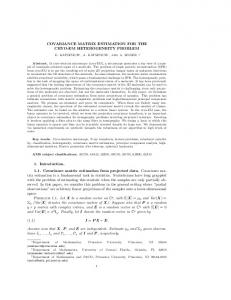
COVARIANCEMATRIXESTIMATIONWITH SPATIALLYDEPENDENT PANEL DATA FIGURE 1.-COVERAGE

RATES FOR NOMINAL

95% CONFIDENCE INTERVALS

g

_SCC

= 100)

~0 0.13

SUR (T= 10)

LS

SUR (T= 100) 0 a

CD

C0

Size of Cross-SectionalDimension (N) Notes: Figure 1 plots the fractionof times a nominal95% confidence ititervalcontainsthe true value of f3 over 1000 Monte Carlo replications, for the indicated N and T. The alternative estimators are as discussed in section IIIB: ordinaryleast squares (OLS), seemingly-unrelatedregressions restrictingthe slope coefficient to be equal across cross-sectional units (SUR), and the spatial correlationconsistent standarderrorsproposedin this paper(SCC).

moderate time-series dimension of size T = 25 and a moderate cross section of N = 20, and describes how the alternative standarderrorestimators discussed perform for a range of values of the spatial and temporal dependence. The left-hand side of table 1 presents the average value over 1000 replications of the various standard error estimators, expressed as a fraction of the sample standard deviation of the point estimator of .20 For consistent estimators such as SUR when p = 0 or the spatial correlation consistent estimator, this ratio should be close to 1, whereas values less than (greater than) 1 indicate downward (upward) finite sample bias. For inconsistent estimators such as OLS in the presence of spatial dependence or SUR when p 0 0, we expect this ratio to differ from 1 in all samples. The right-hand side of table 1 summarizes the consequences for inference of these biases by reporting the fraction of times a nominal 95% confidence interval contains the true value

of ,B. Table 1 reveals that the OLS and SUR estimators exhibit substantial downward bias in the presence of spatial dependence. Even for moderate values of the spatial dependence, the OLS standarderror estimator is biased downward by a factor of about 0.5, and the SUR estimator exhibits even greater downward bias even when it is specified correctly (when p = 0). This downward bias worsens as the temporal dependence increases. In contrast, the spatial correlation consistent standard error estimator displays relatively little finite sample bias, attaining between 92% and 94% of its true value in the case of no temporal dependence, and slightly worse as the temporal dependence increases. The poor performance of the OLS and SUR estimators is mirroredin the coverage rates reportedin the right-handside of table 1. The coverage rates associated with the spatial correlation consistent standard error estimator are between 20 The simulations were run using the random number generator in Gauss 3.2. The autoregressive process for the factors was initialized with a draw from the distribution of ui,.

555

80% and 90% when there is spatial dependence, whereas the OLS and SUR standard error estimators result in coverage rates ranging from about 35% to 60%. However, the superior performance of the spatial correlation consistent standarderror estimator comes at a price. As shown in the upper third of table 1, the spatial correlation consistent standarderrorestimator is dominated by the OLS estimator when there is no spatial dependence. In this case, the consistent OLS estimator displays only modest finitesample bias, while the spatial correlation consistent estimator exhibits slightly greater downward bias. However, we shall see shortly that increasing the length of the time-series dimension does much to improve the performance of the spatial correlation consistent standarderrorestimator. In any case, given the much better performance of this estimator relative to alternatives when there is even modest spatial dependence in the data, this appears to be a small price to pay in return for the greater versatility of the spatial correlation consistent estimator.21 It is worth noting that, although the inconsistent OLS standard error estimator exhibits downwards bias in the presence of spatial dependence in our simulations, the sign of the bias is not a general result. Rather, it is a consequence of our data generating process, which introduces only positive off-diagonal elements into the cross-sectional correlation matrix. Since, loosely speaking, the OLS estimator will not take into account the contribution of these positive elements to the variance of the slope estimator, it will exhibit a downward bias.22If, on the other hand, the cross-sectional correlations take on both positive and negative values but average to zero, then corrections for spatial dependence will not result in variance estimates that are substantially different from uncorrected estimators.23However, this does not 21 We also note this problemis not unique to our spatial correlation consistentestimator.For example, in his comprehensivesurvey of the alternativeheteroskedasticityand autocorrelationconsistentcovariance matrixestimators,Andrews(1991) notes thatcorrectlyspecifiedparametlic estimatorsdominatenonparametric estimatorsin a time-seriessetting. 22 The downwardbias in the SUR estimatoris not a consequenceof our assumptionof positive spatial dependence.Rather, it is due to the feasibility problems of estimatorswhich requirepositive semidefinite estimatesof thecovariancematrix.As N becomeslargefor a fixedvalueof T, the estimatedcovariancematrixbecomes "nearly"singular,and it is to show thatthis introducesdownwardsbias into standard straightforward errorestimates. 23 We also performed oursimulationsdrawingthe factorloadingsfroma uniform distributionwith support(-1, 1), so that the cross-sectional correlationsaveragedto zero. In this case, the performanceof the OLS estimatorswas unaffectedby the presenceof spatialdependence,for the reasonsgiven in the text. It is interestingto note that,as an artifactof the factor structurewe use to introducespatialdependence,includingtime dummiesin the OLSregressionsreportedherewouldhavea similareffect. of takingdeviationsfromperiodmeans This is becausethe transformation would result in a similar factor structure,but with demeanedfactor loadings.Since the demeanedfactorloadingsby constructionaverageto zero, this yields similarresultsto drawingthe factorloadingsfrom the interval(-1, 1). However,this too is not a generalresult.Whenthereare arbitrarycross-sectionalcorrelationsin the residuals,taking deviations from peliod meanswill not reducethe averagevalue of the off-diagonal elements of the covaiiance matrix of the residuals, and hence time dummieswill not mitigatethe problemof spatialdependence.

556


imply that corrections for spatial correlation are unimportant. In fact, in many empirical applications, it is a priori reasonable to assume that the cross-sectional correlations do not average to zero and are generally positive. Spatial correlations induced by unobserved common shocks will only average to zero if the effects of the shocks are purely redistributive. Moreover, we will see in the empirical examples that follow that the spatial correlation consistent standard errors are generally larger than the uncorrected estimates, indicating that the off-diagonal elements of the covariance matrix are in fact generally positive. Thus far we have only considered how the performance of the various estimators depends on the presence of spatial and temporal dependence in the data. We now turn to the question of how the finite-sample properties of these estimators depend on the size of the cross-sectional and time-series dimensions. Figure 1 plots the coverage rates associated with nominal 95% confidence intervals constructed using the three estimators under consideration for time dimensions of T = 10, 50, and 100 and cross-sectional dimensions ranging from N = 1 to N = 100, and for the case of p = 0.3 and an average value of the contemporaneous spatial correlations of 0.125.24 It is immediately apparent from figure 1 that, as suggested by the asymptotic theory which relies only on T becoming large, coverage rates based on the spatial correlation consistent standard errors do not depend on the size of the cross-sectional dimension. In contrast, the performance of the OLS and SUR estimators deteriorates rapidly as the size of the cross-sectional dimension increases. Figure 1 also illustrates that for larger values of the time dimension, such as T = 50 and T = 100, the coverage rates based on the spatial correlation consistent estimator improve over those reported in table 1 (on average 0.908 and 0.920, respectively, versus 0.815 in the case of T = 25). Although these coverage rates still fall short of 95%, they unsurprisingly are comparable to the finite sample performance of standardtime-series heteroskedasticity and autocorrelationconsistent standarderror estimators. For example, Andrews (1991) reports coverage rates of 91.5% for the case of T = 128 and p = 0.3, using a slightly different data generating process and a quadratic-spectal kernel (table IV of that paper). Even for very short time dimensions such as T = 10, the spatial correlation consistent estimator manages respectable coverage rates of about 80%, which dominate the two alternatives for all but very small values of N. We conclude from this that in panel data sets where the time series is long enough that the practitionerwould be comfortable reporting standard time-series heteroskedasticity and autocorrelation consistent standard errors, s/he should also be comfortable reporting spatial correlation consistent standarderrors. 24 For values of N and T where T < (N + 1)/2, SUR is infeasible, and coverage rates are not reported.

VI.

Empirical Examples

The Monte Carlo evidence of the preceding section indicates that failing to take into account spatial dependence can have significant effects on estimated standarderrorsand, hence, on inference. In this section we illustrate the point further by comparing spatial correlation consistent standard errors with common alternatives in the context of three empirical examples: tests of purchasing power parity, tests of consumption risk sharing, and estimation of returns to scale. In particular,for each example we compute five sets of standard errors: (1) simple OLS/IV standard errors, (2) White (1980) heteroskedasticity consistent standard errors, which are robust to heteroskedasticity but not serial or spatial correlation, (3) Newey and West (1987) heteroskedasticity and autocorrelation consistent standard errors, which are robust to heteroskedasticity and within-unit serial correlation, but not to contemporaneous and lagged spatial correlation, (4) spatial correlation consistent standarderrors as proposed here, with lag window m(T) = 0 so that they are robust to heteroskedasticity and contemporaneous spatial correlation alone, and (5) spatial correlation consistent standarderrorswithout restricting the lag window to be zero so that they are robust to heteroskedasticity and serial and spatial correlation.25 In all three applications it is reasonable to expect that the data is characterized by heteroskedasticity and serial and spatial correlation. Thus, only the last estimator will yield consistent estimates, while the other three will be inconsistent and may be biased in any direction, depending on the nature of the serial and spatial dependence in the data. Nevertheless, it is useful to compare these alternative estimators because it provides a sense of the relative importance of corrections for heteroskedasticity and spatial and serial dependence in applied contexts. Throughout, we will emphasize two comparisons. Comparing the White (1980) standard errors in (2) with the spatial correlation consistent standarderrorsin (4) illustrates the importance of correcting for contemporaneous cross-unit correlation alone, while comparing (3) and (5) illustrates the importance of allowing for both contemporaneous and and lagged crosssectional dependence, ratherthan only within-unit temporal dependence. A. PurchasingPower Parity A number of empirical tests of purchasing power parity (PPP) are based on regressions of the form ASit= Ot+

3(Ap - AP*)it+

Eit

25 In this panel setting, we compute "conventional" Newey-West standard errors in (3) as follows. First, we construct the usual time-series estimator of SiT for each cross-sectional unit. Under the assumption that the cross-sectional units are independent, it is straightforwardto see that these can be averaged over the N cross sections to obtain a consistent estimator of ST. In both (3) and (5) we set the lag window m(T) = 2.

COVARIANCEMATRIX ESTIMATIONWITH SPATIALLYDEPENDENT PANEL DATA TABLE 2.-PURCHASING

POWER PARITY REGRESSIONS

ForwardRegression

Coefficient (1) OLS StandardErrors StandardErrorsRobust to: (2) Heteroskedasticity (3) Heteroskedasticityand within-unitserial correlation (4) Heteroskedasticityand contemporaneousspatialcorrelation (5) Heteroskedasticityand contemporaneousand lagged spatial correlation(SCC errors)

557

Reverse Regression

Constant Only

Time Effects

Country Effects

Constant Only

Time Effects

Country Effects

1.006 0.010

1.004 0.010

1.022 0.013

0.814 0.008

0.823 0.008

0.726 0.009

0.054 0.041 0.055 0.035

0.055 0.042 0.055 0.035

0.067 0.056 0.068 0.049

0.051 0.051 0.055 0.054

0.053 0.052 0.056 0.053

0.058 0.062 0.062 0.063

Notes: The firstthreecolumns reportresultsfrom estimatingAsit= ot + (Ap - Ap*)it+ vit,where si, is countryi's exchange raterelativeto the U.S. and the independentvariableis the inflationdifferentialbetween the two countries.a is a set of deterministicvariableswhich alternatelycontainsa constant,time dummnies and countrydummies,as indicatedin the threecolumns. The next threecolumns reportresultsfrom reversing the dependentand independentvariables.The firstrow reportspooled time-seriescross-sectionalOLS coefficient estimates;the remainingrows reportalternativestandarderrorestimates as discussed in the text, with the last row representingthe SCC errorsproposedin this paper.All regressionsuse annualdata covering the period 1973 to 1993 and a sample of 107 countries.

where the dependent variable is the percentage change in the nominal exchange rate while the independent variable is the inflation differential with a base country, usually taken to be the United States.26A point estimate of 3 which does not differ significantly from one can be interpreted as evidence in favor of (relative) Ppp.27 We estimate several variants on this equation using annual data for a sample of 107 countries between 1973 and 1993.28 Table 2 presents OLS estimates of ,3, together with alternative estimates of its standarderror.We note first that the simple OLS standarderrors in (1) are much smaller than any of the alternatives. Comparing (2) and (4), however, suggests that in this example correcting for spatial correlation alone has little effect on estimated standarderrors, with the spatial correlation-consistent standard error estimates differing from the White standard errors by at most 7% (0.062 versus 0.058) in the last column. In contrast, allowing for both contemporaneous and lagged spatial dependence appears to be more important. Comparing the Newey-West standarderrors in (3) with the serial and spatial correlation consistent estimators reveals that the latter are as much as 17% smaller than the former (0.042 versus 0.035 in column 2). B. ConsumptionRisk Sharing Many empirical tests of consumption risk sharing are based on the intuition that, if markets are complete, individual consumption growth should be correlated only with aggregate shocks to income, since individuals are able to

TABLE 3.-CONSUMPTION

RISK-SHARING REGRESSIONS

53 Countries

Coefficient (1) OLS StandardErrors StandardErrorsRobust to: (2) Heteroskedasticity (3) Heteroskedasticity and within-unitserial correlation (4) Heteroskedasticity and contemporaneous spatialcorrelation (5) Heteroskedasticity and contemporaneous and lagged spatial correlation(SCC errors)

OECD (22 countries)

1961-90

1971-90

1960-90

1971-90

1.001 0.020

1.058 0.025

0.773 0.031

0.836 0.041

0.041 0.046

0.052 0.055

0.044 0.052

0.052 0.057

0.037

0.044

0.048

0.070

0.046

0.043

0.045

0.081

Notes: This table reportsthe resultsfrom estimatingAlncj,= 0(t) + 3Axj + Ejt,where the independent variableis growthin consumptionof countryj, 0(t) is a conformablevector of time dummies,and xjtis the idiosyncraticcomponent of GDP growth in countryj, defined as the difference between its growth and growth in world average per capita GDP. The first row reportspooled time-series cross-sectional OLS coefficient estimates; the remainingrows reportalternativestandarderrorestimates as discussed in the text, with the last row representingthe SCC errorsproposedin this paper.All dataare drawnfromthe Penn WorldTables,Version5.6.

diversify away all idiosyncratic income risk. Here we consider an example of such a test based on Lewis (1996), who estimates the following regression: A ln cj,= 0(t) +

xjt

+Ejt

where cjtis consumption in countryj at time t, 0(t) is a vector of time dummies, and xjtis an idiosyncratic shock to income, defined as the deviation of GDP growth in countryj at time t from world average GDP growth. An estimate of ,3 that does not differ significantly from zero can be interpreted as evidence in favor of consumption risk sharing. Table 3 presents the results of estimating this equation for samples of 22 and 53 countries over the period from 1960 to 1990, using OLS.29 In this example, allowing for contemporaneous cross-sectional dependence has larger effects on esti-

26 Herewe follow the notationof FrankelandRose (1996). Fora survey of the empiricalevidenceon PPP,see FrootandRogoff(1995). 27 However,as discussedin FrankelandRose (1996) andelsewhere,the alternativehypothesisdoes nothave an economicallymeaningfulinterpretation. Tests for mean reversion in real exchange rates provide an alternativeframeworknot subjectto this criticism.See FrankelandRose (1996), Wei andParsley(1995), andO'Connell(1998) for examples.The paperby O'Connellis particularlyrelevanthere as it considersthe power of panelunitroottestsin the presenceof cross-sectionaldependence. 28 The exchangerateandinflationdataaredrawnfromthe International MonetaryFund'sInternational FinancialStatistics.Inflationis measuredas 29 Following Lewis (1996), we take all countriesin the Penn World the changein the logarithmof the consumerprice index. The sampleof countriesis restrictedto a sampleof 107 countriesfor whichcompletedata Tableswith dataqualityC+ or better,and restrictour attentionto those areavailablebetween1973and 1993. countrieswithno missingobservationsbetween1960and 1990.


558

TABLE 4.-RETuRNS

TO SCALE IN U.S.

MANUFACTURING INDUSTRIES

3SLS Estimation Method Instrument Set Coefficient (1) 2SLS/3SLS Standard Errors Standard Errors Robust to: (2) Heteroskedasticity and within-unit serial correlation (3) Heteroskedasticity and contemporaneous (4) Heteroskedasticity spatial correlation and contemporaneous and lagged spatial (5) Heteroskedasticity correlation (SCC errors)

I

II

2SLS III

I

II

III

1.120 0.057

1.143 0.056

1.048 0.063

1.312 0.104

1.497 0.095

1.334 0.115

0.096 0.100 0.142 0.185

0.088 0.090 0.108 0.091

0.125 0.124 0.144 0.114

0.100 0.104 0.182 0.195

0.093 0.095 0.141 0.102

0.137 0.137 0.218 0.124

Notes: This table reportsresultsfrom estimatingAvit= yFAX,t + Aait,where the dependentvariableis growthin value addedfor industryi and the independentvariableis growthin a cost-weightedindex of inputs. ThereareN = 20 industriesandT = 32 years (1953-1984). The instrumentsets are as follows: I-real growthin militaiy expenditures,the political partyof the president,andthe worldprice of oil, plus one lag of each; II-only the contemporaneousvalues of I; andIII-instrument set I augmentedwith four lagged values of monetaryshocks, as describedin more detail in Burnside(1996). The firstthreecolumns of resultsarebased on three-stage-least-squaresestimates. The last three columns are two-stage-least-squaresestimates. The first row reportscoefficient estimates, while the remainingrows reportalternativestandarderrorestimates as discussed in the text, with the last row representingthe SCC standarderrorsproposedin this paper.

and the four remaining alternatives (2)-(5) as before. Since 3SLS point estimates incorporate information in the (possibly poorly) estimated cross-sectional covariance matrix, we also report point estimates obtained using 2SLS and the corresponding standarderrors.32Given that in this example the cross-sectional units are industries within a single country and are thus very likely to be subject to common shocks, it is not surprising that corrections for spatial correlation have large effects on estimated standard errors. As before, the importance of correcting for contemporaneous spatial dependence can be seen by comparing the heteroskedasticity consistent White standard errors in (2) with the heteroskedasticity and contemporaneous spatial correlation consistent standarderrors in (4). In all cases the latter are larger than the former, and by as much as 82% in C. Returnsto Scale in U.S. ManufacturingIndustries the case of column 4 of table 4 (0.182 versus 0.100). Lagged The existence of increasing returnsto scale has important cross-sectional dependence also figures prominently, as implications for many branches of macroeconomics. In shown by a comparison of the standarderrorsin (3) and (5), recent years an empirical literature has emerged which with spatial correlation consistent standarderrorsas much as attempts to estimate the degree of returns to scale using 88% higher in the case of column 4 (0.195 versus 0.104). regressions of the form V. Conclusions

mated standard errors. For the 1971-1990 subsample, the spatial correlation consistent standarderrors in (4) are 35% larger than the White standard errors in (2) for the OECD sample (0.070 versus 0.052), and 15% smaller in the full sample of 53 countries (0.044 versus 0.052). Comparing the estimated standarderrorsin (5) and (3) reveals that allowing for contemporaneous and lagged spatial dependence in addition to within-unit serial correlation has even greater effects on estimated standard errors. In the OECD sample over the period of 1971-1990, the spatial correlation consistent standard errors are 42% larger than the Newey-West standarderrors (0.081 versus 0.057), while in the 53-country sample they are 22% smaller (0.043 versus 0.055).

AVit=

yFAX,t + Aait

Spatial and other forms of cross-sectional correlation are to be an important complicating factor in many likely where Avit is growth in value added of industry i, Axit is studies. Standard techniques which fail to take empirical growth in a cost-weighted index of inputs, and Aai, is into account this spatial dependence will lead to inconsistent unobserved growth in productivity.30A point estimate of _yF standard error estimates. Moreover, available techniques that is significantly greater than (less than) 1 can be that in are robust to the presence of spatial principle interpreted as evidence of increasing (decreasing) returns. correlation are often either infeasible or else have poor finite We estimate variants on this specification using a data set In this paper, we have shown that a sample properties. in covering 20 manufacturing subsectors the United States between 1953 and 1984, using various sets of instruments.31 simple transformationof the orthogonality conditions which Table 4 contains the results of these regressions. In the identify a broad class of panel data models permits consisfirst panel we present point estimates obtained using three- tent covariance matrix estimation in the presence of very stage least squares (3SLS), ordinary 3SLS standard errors, general spatial dependence. Moreover, in contrast to existing techniques, the size of the cross-sectional dimension does 30Here we follow the notationof Bumside (1996). See Caballeroand Lyons(1989, 1992),Hall(1988, 1990),BasuandFernald(1995), andBasu (1996) for furtherexamples. 31 The data and instrumentsare describedin more detail in Bumside (1996). We aregratefulto CraigBumsidefor kindlyprovidingus with the dataset andhis programs.The datawereoriginallyconstructedby Robert Hall,to whomthanksarealso due.

32 To be precise,the spatialcorrelation consistentstandarderrorestimatoris constructedas follows:First,we constructeda sequenceof R-vectors of estimatedorthogonalityconditionsby takingthe cross-sectionalaverages of the productsof the instrumentsand either the 2SLS or 3SLS residuals.We then appliedthe Newey-Westestimatorto this sequenceof cross-sectionalaverages.

COVARIANCEMATRIXESTIMATIONWITH SPATIALLYDEPENDENT PANEL DATA not constrain the feasibility of the estimator proposed here. Monte Carlo experiments demonstrate that the finite-sample properties of this estimator are quite good, and are superior to those of other commonly used techniques. We demonstrated the empirical relevance of corrections for spatial dependence through a number of examples in which spatial correlation consistent standard errors differ substantially from those obtained using conventional methods. Finally, we note that this paper has relied exclusively on large T asymptotics to deliver consistent covariance matrix estimates in the presence of cross-unit correlations. However, when T is small or when there is only a single cross section, the problem of consistent nonparametriccovariance matrix estimation appears to be much less tractable. The reason for this is that, unlike in the time dimension, there is no natural ordering in the cross-sectional dimension upon which to base mixing restrictions, and hence it is not possible to construct the pure cross-sectional analogs of nonparametric time-series covariance matrix estimators. Thus it would appear that consistent covariance matrix estimation in models of a single cross section with spatial correlations will have to continue to rely on some prior knowledge of the form of these spatial correlations.

559

Froot,KennethA., and K. Rogoff, "Perspectiveson PPP and Long-Run Real ExchangeRates," in Gene Grossmanand KennethRogoff (eds.), The Handbook of International Economics, vol. 3 (Amster-

dam:NorthHolland,1995). Hall, RobertE., "TheRelationbetweenPrice and MarginalCost in U.S. Industry,"Journal of Political Economy 96 (Oct. 1988), 921-947.

Propertiesof Solow'sProductivityResidual,"in Peter "Invariance Diamond (ed.), Growth/Productivity/Employment(Cambridge, MA:

MITPress),1990,71-112. Hamilton,James D., Time Series Analysis (Princeton,NJ: Princeton UniversityPress,1994). Hansen,Lars P., "LargeSample Propertiesof GeneralizedMethod of MomentEstimators," Econometrica50 (July1982), 1029-1054. Judge,GeorgeG., W. E. Griffiths,R. CarterHill, HelmutLiitkepohl,and Tsoung-Chao Lee, The Theory and Practice of Econometrics (New

York.Wiley,1985). Keane, Michael, and David Runkle, "Testingthe Rationalityof Price Forecasts:EvidencefromPanelData,"AmericanEconomicReview 80 (Sept. 1990),715-735. Kraay,Aart, and JaumeVentura,"Tradeand Fluctuations,"manuscript, WorldBankandMIT(1997). Lehmann,Bruce, "ResidualRisk Revisited,"Journal of Econometrics 45(July-Aug.1990),71-97. Lewis, Karen, "WhatCan Explainthe ApparentLack of Intern?ational Consumption Risk Sharing,?" Journal of Political Economy 104

(Apr.1996),267-297. McLeish, Donald L., "A Maximal Inequalityand DependentStrong Laws," Annals of Probability 3 (1975), 826-836.

Newey, WhitneyK., and KennethD. West, "A Simple, Positive SemiandAutocorrelation ConsistentCovariDefinite,Heteroskedasticity anceMatrix,"Econometrica55 (May 1987),703-708. O'Connell, Paul, "The Overvaluationof PurchasingPower Parity," Journal of International Economics 44 (Feb. 1998), 1-19.

REFERENCES

Patternsof Growth:Persistencein CrossQuah, Danny, "International CountryDisparities,"manuscript,MIT,Departmentof Economics

Amemiya,Takeshi,AdvancedEconometrics(Cambridge,MA: Harvard (1990). UniversityPress,1985). "ExploitingCross-SectionVariationfor Unit Root Inferencein ConsisAndrews,DonaldW. K., "Heteroskedasticity andAutocorrelation DynamicData,"EconomicsLetters44:1-2 (1994), 9-19. tentCovarianceMatrixEstimation,"Econometrica59 (May 1991), Rosenblatt,M., "CentralLimit Theoremfor StationaryProcesses,"in 817-858. Proc. 6th Berkeley Symposium on Mathematical Statistics and Andrews,Donald W. K., and J. ChristopherMonahan,"An Improved Probability,vol. 2 (1970), 51-561. Heteroskedasticity andAutocorrelation ConsistentCovarianceMa- Wei, S. J., and D. Parsley, "PurchasingPower Disparity during the trixEstimator," Econometrica60 (July1992),953-966. FloatingRatePeriod:ExchangeRateVolatility,TradeBarriersand Anselin,Luc,SpatialEconometrics(Dordrecht: Kluwer,1988). OtherCulprits,"NBERWorkingPaper5032 (1995). Basu, Susanto,"ProcyclicalProductivity:IncreasingReturnsor Cyclical White, Halbert, "A Heteroscedasticity-Consistent CovarianceMatrix Utilization,?" Quarterly Journal of Economics 111, (Aug. 1996), Econometrica Estimatoranda DirectTestfor Heteroscedasticity," 719-752. 44 (Apr.1980),817-838. Basu, Susanto, and J. G. Fernald, "AggregateProductivityand the Asymptotic Theory for Econometricians (New York: Academic Productivityof Aggregates,"NBERWorkingPaper5382 (1995). Press,1984). Bulinskii,A. V., "On VariousConditionsfor Mixing and Asymptotic Wooldridge,JeffreyM., andHalbertWhite, "SomeInvariancePrinciples of RandomFields,"SovietMath.Dokl.37:2(1988)443-448. Normality and CentralLimit Theoremsfor DependentHeterogenousProBurnside,Craig,"ProductionFunctionRegression,Returnsto Scale, and cesses," Econometric Theory 4 (1988), 210-230. Externalities," Journal of Monetary Economics 37 (Apr. 1996), Zellner,Arnold,"AnEfficientMethodof EstimatingSeeminglyUnrelated 177-201. Regressions and Tests of Aggregation Bias," Journal of the Caballero,Ricardo,andRichardLyons,"TheRole of ExternalEconomies American Statistical Association 57 (1962), 348-368. in U.S. Manufacturing," NBERWorkingPaper3033 (1989). "ExternalEffects in U.S. ProcyclicalProductivity,"Journal of Monetary Economics 29 (Apr. 1992), 209-226.

Case,Anne C., "SpatialPatternsin HouseholdDemand,"Econometrica 59 (July1991),953-965. Conley,TimothyG., "EconometricModellingof CrossSectionalDependence,"manuscript,Universityof Chicago(1994). Doukhan, Paul, Mixing: Properties and Examples (New York: Springer,

APPENDIX Proof of Result 1

The proofis simplya matterof verifyingthath, satisfiesthe definition 1994). of univariatemixing. Define B, = {vIv < tl E Z' as the naturaloneElliott, Graham,"SpatialCorrelationsand Cross-CountryRegressions," dimensionalanalogof andsimilarly U( At, E(, z E Bt) and =+S manuscript,HarvardUniversity(1993). Frankel,JeffreyA., andAndrewK. Rose, "A PanelProjecton Purchasing U(E, zE Btc). Define the mixing coefficients for the sequence , as Go2 E S_-s)IP[GI n G2] -P[G1]P[G2 |I. Now we Power Parity:Mean Reversionwithin and between Countries," Oth(s) = SUp(t) SUP(GI E 7?_X and ,+s C ,+s. Given this claim, we have C claim that 39 _X Journal of Intetnational Economics 40 (Feb. 1996), 209-224. in PanelData," Oth(S) C of(s) for all s, andhenceoth(s) convergesat leastas quicklyas cx(s). Frees,EdwardW., "AssessingCross-SectionalCorrelation Thusthe sequencehtis mixingof the samesize of hit. Journal of Econometrics 69 (Oct. 1995), 393-414. RI is a Borel function of To verify the claim, note that ht: fl Froot, Kenneth A., "ConsistentCovarianceMatrix Estimation with in Financial [hiti = 1,..., N,.. .},andhence is a(hit|i 1,..., N,.. .)-measurable, Cross-SectionalDependenceand Heteroskedasticity that is, h-1'(.,) C a(hi = 1,..., N . ), where X is the a-algebra Data," Journal of Financial and Quantitative Analysis 24 (Sept. generatedby the Borel sets. Thus by definitiona(ht) = a(h' c(p))c 1989),333-355.

560


Finally, note that 9t-_x t -=_x N,...). = a(h,) and a(hi,ti= 1. t x ,'= X-xt N,.. .), and so the claim is verified. oxa(hiv i = 1,

Consistencyand AsymptoticNormalityof the GMM Estimator We firstnote thatthe assumptionsof result2 are sufficientto establish consistency of the GMM estimator.The proof consists of verifying standardconditionsfor the consistencyof extremumestimatorssuch as thosein Ameniiya(1985, theorem4.1.1). ConditionsA andB of Amemiya (1985, theorem4.1.1) follow immediatelyfrom assumption(a) of our result2. ConditionC of this theoremrequiresthe minimandin the GMM problemto satisfy a law of largenumbersas T - oo.By result 1 in this paper, ht(O)is a univariatear-mixingsequence of size 2r/(r - 1) > rl(r - 1). Thus to apply the McLeish (1975) LLN (see White (1984, theorem3.47) for cx-mixingsequencesof size rl(r - 1), we need only verify that ht(O)has finite (r + 8)thmoments.This follows immediately from assumption(1), which imposesthe strongercondition(requiredfor consistency of the covariancematrix estimator)that hit(O)has finite 4(r + 8)thmoments,and the fact that ht(O)is the sum of N(T) random variablesnormalizedby N(T). Thus the GMMestimatoris consistentas T - oo. To establishasymptoticnormalityof the GMMestimator,we needonly verify standardconditionssuch as those in Hamilton(1994, proposition 14.1) (which are in turnadaptedfrom Hansen(1982)). Condition(a) of Hamilton(1994, proposition14.1) follows from the consistencyof the GMMestimator.To verify condition(b) of Hamilton(1994, proposition 14.1), we need to show that the sequenceht(O)satisfies a centrallimit theoremfor dependentprocessessuchas White(1984, theorem5.19).This theoremrequiresht(O)to be an aL-mixing sequenceof size rl(r - 1) with finite2rthmoments.Boththeseconditionshavebeenverified.In addition,

this centrallimit theoremrequiresthe assumptionof asymptoticcovariance stationarity, Var[T-1"21 ia+TIh, (0)] V - 0 uniformlyin a as T -o for V positive definite.If we make this assumption,togetherwith the regularityconditionon the partialderivativesof hit(O)in condition(c) of Hamilton(1994, proposition14.1), asymptoticnormalityof the GMM estimator as T -

oois immediate.

One remarkon the covariancestationarityassumptionrequiredfor asymptoticnormalityis in order.If the cross-sectionaldependenceis sufficientlyweak and if N(T) grows quickly enough relativeto T, the conditionthatVbe positivedefinitemaynothold.To see this,notethat 1

a+T

1ar T

E t=a+l

a+T

a-T

1

N(T) N(T)\

,()=Tt=a?+ s=a+?1 N(T)i

E [hit(O)hjs(0)]| 1 j=1

1

If thecross-sectionaldependenceis weakin the sensethatthe innerdouble sum over the cross-sectionsof the cross-sectionalcovariancesis of order less thanN(T)2,say,for example,N(T)2-2E, andif N(T) growsfastenough relativeto T, thenit is possiblethatV = 0 sincethe termin theparentheses vanishesas N(T) becomes large.However,this point need not detainus since it simply amountsto an observationthat if the cross-sectional dependenceis nottoo strong,theGMMestimatorconvergesin distribution at a rate fasterthan T1/2. In particular,if we replaceht(0) with gt(0) = N(T)Eh,(0)in the precedingarguments,asymptoticnormalityof the GMM estimatoris immediate.Thus the estimatoris asymptoticallynormalat least at rateT1"2,andthe weakerthe cross-sectionaldependence(i.e., the largeris e), the fasteris the rateof convergence.Theproofsof consistency of the GMMestimatorandconsistencyof the covariancematrixestimator areunaffectedby thispoint.