Consistent Dynamic Process Models

Five Steps for Building

Consistent Dynamic Process Models and their Implementation in the Computer Tool Modeller

CIP-DATA LIBRARY TECHNISCHE UNIVERSITEIT EINDHOVEN

Westerweele, Mathieu R.

Five steps for building consistent dynamic process models : and their implementation in the computer tool Modeller / by Mathieu R. Westerweele.Eindhoven : Technische Universiteit Eindhoven, 2003. Proefschrift. - ISBN 90-386-2964-8 NUR 913 Trefwoorden: procesregeling en dynamica / chemische technologie; fysischchemische simulatie en modellering / dynamische simulatie; methodologie / wiskundige modellen / computerapplicatie; algoritme Subject headings: process control and dynamics / chemical engineering; physicochemical simulation and modelling / dynamic simulation; methodology / mathematical models / computer application; algorithm

Omslag: Govert Sleegers Druk: Universiteitsdrukkerij TU Eindhoven, The Netherlands

c 2003 by M.R.Westerweele Copyright ° All rights reserved. No parts of this publication may be reproduced or utilized in any form or by any means, electronic or mechanical, including photocopying, recording or by any information storage and retrieval system, without permission of the copyright holder.

Five Steps for Building

Consistent Dynamic Process Models and their Implementation in the Computer Tool Modeller

PROEFSCHRIFT

ter verkrijging van de graad van doctor aan de Technische Universiteit Eindhoven, op gezag van de Rector MagniÞcus, prof.dr. R.A. van Santen, voor een commissie aangewezen door het College voor Promoties in het openbaar te verdedigen op maandag 14 april 2003 om 16.00 uur

door

Mathieu Ruurd Westerweele

geboren te Oostburg

Dit proefschrift is goedgekeurd door de promotoren:

prof.dr.Dipl-Ing. H.A. Preisig en prof.dr.ir. A.C.P.M. Backx

THERE IS NO TIME LIKE THE PRESENT Mark Twain said, ”I have been through some terrible things in my life, some of which actually happened”. These words hold great wisdom; the wisdom of knowing that there is no sense worrying about the past or fearing the future. Your past will not change, and your future concerns may never come. Many people spend a great deal of time and energy thinking about past problems and future concerns, while the present is passing them by. Remember the here and now is a gift, which is why they call it the ’present’. Treat it like a present, enjoy it to the fullest and make the most of it. Don’t let your life pass you by, focus on the present and enjoy today! - Glen Hopkins

vi

Contents Summary

xi

Voorwoord

xiii

1 Introduction 1.1 Motivation and Goals . . . . . . . 1.2 Application Dependency of Models 1.3 Structured Modelling Methodology 1.4 Overview of Related Work . . . . . 1.5 Scope of this Project . . . . . . . . 1.6 Outline and Intention of the Thesis

I

. . . . . .

. . . . . .

. . . . . .

. . . . . .

. . . . . .

. . . . . .

. . . . . .

. . . . . .

. . . . . .

. . . . . .

. . . . . .

. . . . . .

. . . . . .

. . . . . .

. . . . . .

. . . . . .

Modelling Methodology

1 1 4 5 7 9 10

13

2 Introduction to Modelling 2.1 Three Principal Problems . . . . . . . . 2.2 The Modelling Process . . . . . . . . . . 2.3 Formulation of the Model . . . . . . . . 2.3.1 Primary Modelling Operation . . 2.3.2 Assumptions about the Nature of

. . . . . . . . . . . . . . . . . . . . . . . . . . . . the Process

. . . . .

. . . . .

. . . . .

. . . . .

. . . . .

. . . . .

15 15 17 18 18 20

3 Hierarchical Organisation: The Physical 3.1 Building Blocks . . . . . . . . . . . . . . 3.2 Domains . . . . . . . . . . . . . . . . . . 3.3 Fundamental Time Scale Assumptions . 3.4 Hierarchical Organisation . . . . . . . .

Topology . . . . . . . . . . . . . . . . . . . . . . . . . . . .

. . . .

. . . .

. . . .

. . . .

. . . .

. . . .

21 21 26 27 33

4 Chemical Distribution: The Species Topology 39 4.1 Chemical Distribution . . . . . . . . . . . . . . . . . . . . . . . 39 4.2 Permeability of Mass Connections . . . . . . . . . . . . . . . . 40 4.3 Uni-directionality of Mass Connections . . . . . . . . . . . . . . 42 vii

viii

Contents 4.4

Reactions . . . . . . . . . . . . . . . . . . . . . . . . . . . . . .

5 Mathematical Description: The Equation Topology 5.1 Variable ClassiÞcation . . . . . . . . . . . . . . . . . . 5.1.1 System Variables . . . . . . . . . . . . . . . . . 5.1.2 Connection Variables . . . . . . . . . . . . . . . 5.1.3 Reaction Variables . . . . . . . . . . . . . . . . 5.2 Fundamental State Variables and Equations . . . . . . 5.3 Balance Equations . . . . . . . . . . . . . . . . . . . . 5.3.1 Mass Balances . . . . . . . . . . . . . . . . . . 5.3.2 Energy Balances . . . . . . . . . . . . . . . . . 5.3.3 Conclusions . . . . . . . . . . . . . . . . . . . . 5.4 Algebraic Equations . . . . . . . . . . . . . . . . . . . 5.4.1 System Equations . . . . . . . . . . . . . . . . 5.4.2 Connection Equations . . . . . . . . . . . . . . 5.4.3 Reaction Equations . . . . . . . . . . . . . . . 5.4.4 Summary . . . . . . . . . . . . . . . . . . . . . 5.5 Linear and Linearised Models . . . . . . . . . . . . . . 5.5.1 Linearisation . . . . . . . . . . . . . . . . . . . 5.5.2 State Space Description for Linear Models . . . 5.5.3 State Space Description for Linearised Models . 5.6 Substitution, yes or no? . . . . . . . . . . . . . . . . . 5.7 Control . . . . . . . . . . . . . . . . . . . . . . . . . . 6 Assumptions: Problems and Solutions 6.1 High-index Models . . . . . . . . . . . . . . . . . 6.2 Assumptions Leading to High-index Models . . . 6.3 Index Reduction Algorithms . . . . . . . . . . . . 6.3.1 Simple Index Reduction Algorithm . . . . 6.3.2 Full Index Reduction Algorithm . . . . . 6.4 Steady-State Assumptions . . . . . . . . . . . . . 6.5 Events and Discontinuities . . . . . . . . . . . . . 6.6 Variables and Algebraic Equations for Composite 6.7 Summary and Conclusions . . . . . . . . . . . . .

II

Implementation

. . . . . . . . . . . . . . . . . . . .

. . . . . . . . . . . . . . . . . . . .

. . . . . . . . . . . . . . . . . . . . . . . . . . . . . . . . . . . Systems . . . . .

. . . . . . . . . . . . . . . . . . . .

. . . . . . . . .

. . . . . . . . . . . . . . . . . . . .

. . . . . . . . .

42

. . . . . . . . . . . . . . . . . . . .

43 44 44 45 46 47 48 48 55 58 59 59 62 63 64 65 65 67 71 73 74

. . . . . . . . .

77 78 79 80 81 84 89 94 98 99

103

7 Introduction to Implementation 105 7.1 Implementation Details . . . . . . . . . . . . . . . . . . . . . . 107

Contents

ix

8 Construction of the Physical Topology 8.1 Handling Complexity . . . . . . . . . . . . . . . . . . . . . 8.2 Unique System IdentiÞers . . . . . . . . . . . . . . . . . . 8.3 Basic Tree Operations . . . . . . . . . . . . . . . . . . . . 8.4 Representation of Connections . . . . . . . . . . . . . . . 8.4.1 Making a New Connection . . . . . . . . . . . . . . 8.4.2 Graphical Representation of Connections . . . . . 8.5 Consequences of Manipulations on the Physical Topology 8.5.1 Loose Connections . . . . . . . . . . . . . . . . . . 8.5.2 Open Connections . . . . . . . . . . . . . . . . . . 8.5.3 Possible States of Connections . . . . . . . . . . . 8.6 Repetitive Structures . . . . . . . . . . . . . . . . . . . . .

. . . . . . . . . . .

. . . . . . . . . . .

. . . . . . . . . . .

111 111 113 114 119 120 120 123 123 125 126 127

9 Construction of the Species Topology 9.1 DeÞning Plant Species and Reactions . . . . 9.2 Injecting Species and Reactions . . . . . . . 9.3 Permeability and Uni-Directionality of Mass 9.4 Propagation of Species . . . . . . . . . . . . 9.5 Consequences of Manipulations . . . . . . .

. . . . .

. . . . .

. . . . .

131 131 132 134 135 141

. . . . . .

143 143 146 148 156 156 156

10 Construction of the Equation Topology 10.1 Balance Equations . . . . . . . . . . . . 10.2 Equation ClassiÞcation . . . . . . . . . . 10.3 Computational Order . . . . . . . . . . 10.4 Output of Modeller . . . . . . . . . . . . 10.4.1 Documentation File . . . . . . . 10.4.2 Code File . . . . . . . . . . . . .

III

. . . . . .

. . . . . .

. . . . . . . . . . . . . . . . Connections . . . . . . . . . . . . . . . .

. . . . . .

. . . . . .

. . . . . .

. . . . . .

. . . . . .

. . . . . .

. . . . . .

. . . . . .

. . . . . .

. . . . . .

Examples and Conclusions

11 Examples 11.1 Tank With Level Measurement . . . . . . . . . . . . 11.1.1 Problem Description . . . . . . . . . . . . . . 11.1.2 Step 1: Physical Topology . . . . . . . . . . . 11.1.3 Step 2: Species Topology . . . . . . . . . . . 11.1.4 Step 3: Balance Equations . . . . . . . . . . . 11.1.5 Step 4a: Connection and Reaction Equations 11.1.6 Step 4b: System Equations . . . . . . . . . . 11.1.7 Discussion . . . . . . . . . . . . . . . . . . . . 11.2 Extraction Process . . . . . . . . . . . . . . . . . . . 11.2.1 Problem Description . . . . . . . . . . . . . .

159 . . . . . . . . . .

. . . . . . . . . .

. . . . . . . . . .

. . . . . . . . . .

. . . . . . . . . .

. . . . . . . . . .

161 162 162 162 163 163 163 164 165 166 166

x

Contents 11.2.2 Step 1: Physical Topology . . . . . . . . . . . 11.2.3 Step 2: Species Topology . . . . . . . . . . . 11.2.4 Step 3: Balance Equations . . . . . . . . . . . 11.2.5 Step 4a: Connection and Reaction Equations 11.2.6 Step 4b: System Equations . . . . . . . . . . 11.2.7 Discussion . . . . . . . . . . . . . . . . . . . . 11.3 Dynamic Flash . . . . . . . . . . . . . . . . . . . . . 11.3.1 Problem Description . . . . . . . . . . . . . . 11.3.2 Step 1: Physical Topology . . . . . . . . . . . 11.3.3 Step 2: Species Topology . . . . . . . . . . . 11.3.4 Step 3: Balance Equations . . . . . . . . . . . 11.3.5 Step 4a: Connection and Reaction Equations 11.3.6 Step 4b: System Equations . . . . . . . . . . 11.3.7 Discussion . . . . . . . . . . . . . . . . . . . . 11.4 Distillation Column . . . . . . . . . . . . . . . . . . 11.4.1 Problem Description . . . . . . . . . . . . . . 11.4.2 Step 1: Physical Topology . . . . . . . . . . . 11.4.3 Step 2: Species Topology . . . . . . . . . . . 11.4.4 Step 3: Balance Equations . . . . . . . . . . . 11.4.5 Step 4a: Connection and Reaction Equations 11.4.6 Step 4b: System Equations . . . . . . . . . . 11.4.7 Discussion . . . . . . . . . . . . . . . . . . . .

12 Conclusions and Future Work 12.1 Conclusions . . . . . . . . . . . . . . . . . . . . . . 12.1.1 Systematic Modelling Methodology . . . . . 12.1.2 Minimal Representation of Process Models 12.1.3 Automatic Documentation of Assumptions 12.1.4 Local Handling of Assumptions . . . . . . . 12.1.5 Education . . . . . . . . . . . . . . . . . . . 12.2 Suggestions for Further Research . . . . . . . . . . 12.2.1 Modelling . . . . . . . . . . . . . . . . . . . 12.2.2 Implementation . . . . . . . . . . . . . . . .

. . . . . . . . .

. . . . . . . . . . . . . . . . . . . . . .

. . . . . . . . . . . . . . . . . . . . . .

. . . . . . . . . . . . . . . . . . . . . .

. . . . . . . . . . . . . . . . . . . . . .

. . . . . . . . . . . . . . . . . . . . . .

. . . . . . . . . . . . . . . . . . . . . .

166 167 168 169 170 170 172 172 173 173 174 176 177 178 179 179 179 180 181 181 181 182

. . . . . . . . .

. . . . . . . . .

. . . . . . . . .

. . . . . . . . .

. . . . . . . . .

. . . . . . . . .

183 183 183 186 187 187 188 188 189 190

Bibliography

193

A Module CamTools

201

B Example of Modeller Output Files

205

Samenvatting

212

Curriculum Vitae

215

Summary The main goal of this research project was the development of a systematic modelling method for the design of Þrst principles based (i.e. based on physical insight), dynamic process models for macroscopic physical, chemical and/or biological processes. The modelling of such processes is one of the most important tasks of a process engineer, for these models are used on a large scale for all kinds of engineering activities, such as process control, opimisation, simulation, process design and fundamental research. The construction of these models is, in general, seen as a difficult and very time consuming task and is preferably handed over to ”modelling experts”. This does not have to be the case if a clear, stepwise method is adhered to. The modelling methodology is based on the hierarchical decomposition of processes into thermodynamic systems and consists of Þve steps: (i) Subdivide the process into smaller parts, that can be easily (mathematically) described individually. In this step, the so-called Physical Topology is constructed, using only two basic building blocks, namely Systems, which represent capacities that are able to store the fundamental extensive quantities (such as component mass, energy and momentum), and Connections, which describe the transfer of these fundamental extensive quantities through the common boundaries of the interconnected systems. (ii) Construct the Species Topology. The Species Topology describes the distribution of all involved chemical and/or biological species as well as all their transformation into other species in the various parts of the process. (iii) For each relevant extensive quantity (such as, for example, component mass or energy) of each system write the corresponding balance equations. (iv) Augment the model equations with deÞnitions and equations of state and choose the transfer laws and kinetic laws that express the ßow and production rates (present in the balance equations). Also deÞne possible constraining assumptions (i.e. ”simpliÞcations” that may lead to highindex DAEs (Differential Algebraic Equations)). The resulting mathematical problems can always be resolved by applying a model reduction. (v) Add the dynamic behaviour of the information processing units, such as controllers. These steps for building a model do not have to be done strictly in this xi

xii

Summary

sequence - at least not for the overall model. It is left to the model designer when the details are being speciÞed in each part of the model. This Þve step procedure of building dynamic process models always results in a differential algebraic system with an index of one. The model can be used for solving certain problems related to the process or it can be further modiÞed by applying mathematical manipulations, such as linearisation or model reduction. An other important goal of this project was the implementation of the modelling methodology into a new computer tool, called ”The Modeller”. This tool is designed to effectively assist a model designer with the construction of consistent process models and to (signiÞcantly) reduce the needed time and overall effort. With the modelling tool, the process models can be built using two main operations, namely reÞning existing systems (the top-down approach) or grouping systems (the bottom-up approach). These two operations can be used interchangeably and all performed actions can be undone (multiple undo/redo mechanism). The software allows to store, retrieve, import or export models (or parts of models) at any stage of the model deÞnition. This allows for a safe mechanism of model reuse. The computer tool is implemented with BlackBox Component Builder 1.4 (Component Pascal), which is a component oriented programming language comparable to Java.

Voorwoord ”Het duurt even, maar dan heb je ook wat! ”, zegt men wel eens. Dat gaat ook zeker op voor dit werk: het heeft iets langer geduurd dan gebruikelijk om dit promotiewerk af te ronden, maar het resultaat is een stuk werk waar ik trots op ben en waar ook anderen iets aan zullen hebben. Tijdens mijn onderzoek is een methodiek ontwikkeld waarmee men (veel) sneller dynamische proces modellen kan opstellen, die bovendien ”automatisch” worden gedocumenteerd door het gebruik van deze methode. De ontwikkelde methode is reeds gedeeltelijk ge¨õmplementeerd in het computerprogramma ”MODELLER”, waarmee het effect van de methode zeer goed kan worden gedemonstreerd. Ik heb de afgelopen 5 jaar veel geleerd en daar ben ik vele mensen dankbaar voor. Allereerst natuurlijk een woord van dank aan mijn dagelijkse begeleider en promotor professor Heinz Preisig. Heinz, ik vond het erg plezierig om met je samen te werken. Je was altijd - nou ja, meestal - open voor discussies en hebt me veel geleerd op velerlei gebieden. Ik hoop dan ook het contact niet te verliezen nadat deze promotie is afgerond, zodat er nog veel goede dingen uit een blijvende samenwerking kunnen voortvloeien. Ook mijn copromotor Ton Backx, de leden van de kerncommissie, Okko Bosgra en Wolfgang Marquardt, alsook de overige leden van de promotiecommissie, Costas Pantelides, Piet Kerkhof, Jos Keurentjes en Johan Wijers, wil ik van harte bedanken voor hun steun, interesse, constructieve discussies en feedback. In de eerste jaren van mijn promotieonderzoek was Martin Weiss mijn directe begeleider. Ik heb van hem veel geleerd (vooral op wiskundig gebied) en vind het jammer dat hij er in de latere fase van mijn onderzoek niet meer bij was. Martin, bedankt voor je steun en interessante discussies. Ook de studenten, Steven Grijseels en Reinout Dekkers, die mij in de eerste fase van mijn onderzoek hebben geholpen met het uitzoeken van bepaalde zaken, wil ik hartelijk bedanken voor hun inzet en bijdrage. Naast mijn bijdrage op wetenschappelijk gebied heb ik ook op educatief gebied een steentje proberen bijdragen. Ik wil Henk Leegwater hartelijk bedanken voor de ruime mogelijkheden mezelf op dit gebied te ontwikkelen. Ik xiii

xiv

Voorwoord

heb van deze periode ontzettend veel geleerd en heb daarin ook zeer veel plezier gehad. Ook de student-assistenten, M’hamed, Leo, Frans, Hans-Jan, Hans en Alex, die hebben geholpen het practicum op poten te zetten en te houden, wil ik hartelijk bedanken voor hun enorme inzet. Voor de Þjne werksfeer die rond mij heerste in de eerste fase van mijn onderzoek wil ik graag mijn ex-collega aio’s Annelies, Georgo, Gerwald, Patrick, Roel en Uwe, alsook de overige medewerkers van onze ex-vakgroep, Tiny, Tanja, Thea, Frank, Stefan, Ivonne, Henk, Martin en Heinz, bedanken. In de tweede fase van mijn onderzoek was ik gehuisvest bij de regeltechniek vakgroep van de faculteit electrotechniek. Ik wil deze gehele vakgroep en met name Paul van de Bosch hartelijk bedanken voor hun bereidheid onze groep op te nemen in de hunne alsook voor de plezierige werksfeer tijdens de afronding van mijn promotiewerk. Govert Sleegers wil ik bedanken voor het ontwerpen van de omslag van dit proefschrift. Goof, ondanks dat je waarschijnlijk geen bal van de inhoud van dit proefschrift begrijpt (of wilt begrijpen), vind ik toch dat je er erg goed in geslaagd bent een beeld hiervan te schetsen op de omslag. Hartelijk dank voor het fraaie ontwerp. Voor het wekelijkse vertier in de vorm van squash, pool, spelletjes dan wel muziek wil ik graag Xander, Jip, Bart, Martin, Arjan, Paul, Emiel, Patrick, Ignace, Jan, Edwin, Luc, Ruben, Rogier en de leden van Quadrivium en Bigband de Mooche bedanken alsook alle anderen die me tijdens deze brainstormsessie niet te binnen zijn geschoten. Mijn ouders en schoonouders alsook de rest van mijn familie wil ik hartelijk bedanken voor hun steun, geduld en interesse. Pa en ma, hartelijk bedankt mij de mogelijkheid te bieden zover te kunnen komen. Al mijn aangetrouwde ”broers” en ”zussen”, Frank, Kurt, Mark, John, Annemiek en Bianca, maar in het bijzonder mijn eigen broer en zus, Michel en Esther, wil ik hartelijk bedanken voor hun interesse, steun en vele goede hints. Het laatste bedankje gaat natuurlijk richting de belangrijkste mensen in mijn leven: mijn eigen gezinnetje. Lisanne, Kevin en Nathalie (en zelfs ook ons volgende kindje, die pas over enkele maanden het daglicht voor het eerst zal zien), bedankt voor de vele plezierige momenten en de nodige inspiratie die jullie me hebben bezorgd tijdens mijn promotieperiode. Jullie hebben mijn leven heel wat meer inhoud en kleur gegeven. Mijn belangrijkste steun en toeverlaat was en is natuurlijk mijn vrouw Miranda. Zonder haar geduld, steun en liefde zou ik zeker niet tot zo’n mooi eindresultaat zijn gekomen. Miranda, bedankt voor alles. Ik hoop dat we nog vele jaren gelukkig kunnen verder leven met ons gezin. Mathieu.

Chapter 1

Introduction A chemical engineer is often asked to describe the dynamic and/or static behaviour of a physical-chemical-biological (PCB) process (or a set of these processes, which constitute a plant), because information about this behaviour is needed for operations like analysis, control, design, simulation, optimisation or process operation. In order to analyse the behaviour of such a process, the engineer often needs a mathematical representation of the physical and chemical and/or biological phenomena taking place in it. The representation of a PCB process in form of a mathematical model is the key to many chemical engineering problems (e.g. (Cellier 1991) (Marquardt 1994a)(Ogunnaike 1994)(Hangos and Cameron 2001)). Modelling a chemical process requires the use of all the basic principles of chemical engineering science, such as thermodynamics, kinetics, transport phenomena, etc. It should therefore be approached with care and thoughtfulness (Stephanopoulos 1984).

1.1

Motivation and Goals

A (mathematical) model of a process is usually a system of mathematical equations, whose solutions reßect certain quantitative aspects (dynamic or static behaviour) of the process to be modelled (Aris 1978) (Denn 1986)(Ogunnaike 1994). The development of such a mathematical process model is initiated by mapping a process into a mathematical object. The main objective of a mathematical model is to describe some behavioural aspects of the process under investigation. The modelling activity should not be considered separately but as an integrated part of a problem solving activity. Preisig (Preisig 1991b), (Preisig 1991a) analysed and decomposed the overall task of problem solving into the following set of subtasks: • (Primary) Modelling. The Þrst step in the process of obtaining a 1

2

Introduction process model is the mapping of the ”real-world” into a mathematical object, called the primary model. In doing so, one may take different views and accordingly apply different theories, which naturally will result in different models. Within this Þrst step, assumptions are made about the principle nature of the process (such as time scales of hydraulics and reactions, fundamental states, etc.). • Model manipulation. The model can be simpliÞed by applying mathematical manipulations, such as: — Model reduction — Linearisation — Transformation to alternative representations of the model — re-arrangement of the mathematical problem equations • Problem speciÞcation. Certain variables are instantiated (i.e. deÞned as known), such that they are available later during solution time and such that the number of equations equals the number of unknown variables. • Analysis of the mathematical model. The analysis of the mathematical problem is done in connection with the speciÞcation of the model. On the simple level, a degree of freedom analysis may be done, which for large scale systems is by no means trivial. On the higher level, one may look into things as index of the differential algebraic system. • Solution of the mathematical model. General purpose mathematical packages, such as differential algebraic equation solvers, large scale simulators, linear algebra packages, etc., are used to solve particular problems. • Analysis of the results. The analysis of the results must focus on a veriÞcation of the results by comparing them with known pieces of information. This may be experimental data or just experience.

The outcome of the performance of each task must fulÞl a set of speciÞcations and requirements, otherwise the design is iterated by looping back to any previous task. This implies that modelling is a recursive and iterative process (and that includes not only the modelling, but everything that is associated with the use of the model). Rarely does one in the Þrst attempt obtain a proper model for the problem under investigation. Usually, an adequate model is constructed progressively through a loop comprising a series of tasks of model development and model validation.

1.1 Motivation and Goals

3

More often than not, the time spent on collecting the information necessary to properly deÞne an adequate model is much greater than the time spent by a simulator program in Þnding a solution. Most publications and textbooks present the model equations without a description of how the model equations have been developed. Hence, to learn dynamic model development, novice modellers must study examples in textbooks, the work of more skilled modellers, or use trial and error (Moe 1995). During the last decades there tends to be an increasing demand for models of higher complexity, which makes the model construction even more time consuming and error-prone (MacKenzie and Ponton 1991)(Marquardt 1991)(Marquardt 1992). Moreover, there are many different ways to model a process (mostly depending on the application for which the model is to be used): different time scales, different levels of detail, different assumptions, different interpretations of (different parts of) the process, etc. Thus a vast number of different models can be generated for the same process. All this calls for a systematisation of the modelling process, comprising of an appropriate, well-structured modelling methodology for the efficient development of adequate, sound and consistent process models. Modelling tools building on such a systematic approach support teamwork, re-use of models, provide complete and consistent documentation and, not at least, improve process understanding and provide a foundation for the education of process technology (Bieszczad 2000)(Moe 1995)(Preisig et al. 1991). This work presents the concepts and design of Modeller, a computer-aided modelling tool built on a structured modelling methodology, which aims to effectively assist in the development of process models and helps and directs a modeller through the different steps of this methodology. It was not a project objective to introduce new elements or a new modelling language. The objective of this project is to provide a systematic model design method that meets all the mentioned requirements and turns the art of modelling into the science of model design. The focus of this work is primarily on modelling and not on problem solving. Most of the currently available modelling languages and simulation packages focus on model manipulation, speciÞcation, analysis and/or solution and more or less leave out the modelling part. In general it is assumed that the mathematical model of the process under investigation is known or easy to assemble. The development of process models, however, is slow, error prone and consequently a costly operation in terms of time and money (Sargent 1983)(Asbjørnsen et al. 1989)(Marquardt 1992). Modelling is an acquired skill, and the average user Þnds it a difficult task (Sargent 1989)(Evans 1990). A modeller may inadvertently incorporate modelling errors during the mathematical formulation of a physical phenomenon.

4

Introduction

Formulation errors, algebraic manipulation errors, writing and typographical errors are very common when a model is being implemented in a computing environment. Thus any procedure which would allow to do some of the needed modelling operations automatically would eliminate a lot of simple, low-level (and hard to detect) errors (Preisig 1991c). Modeller is a computer-aided modelling tool which is designed to assist a model designer to map a process into a mathematical model, using a systematic modelling methodology. The task solved by Modeller is purely the construction and manipulation of the structure and deÞnition of process models. The tool is not designed to solve speciÞc problems concerning any model, as such programs (Modelica, gProms, ASCEND, Dymola, SpeedUp, DASSL, DASOLV, DAEPACK, etc.) are already available. The sole task of Modeller is to provide an interface allowing to construct and edit symbolic process models. The output of Modeller is a Þrst-principles based (i.e. based on physical insight (Asbjørnsen et al. 1989)) mathematical model with a minimal realisation, which is easily transformed to serve as an input to existing modelling languages and/or simulation packages, such as gProms, ABACUSS, ASCEND, Modelica, Matlab.

1.2

Application Dependency of Models

This work is concerned with the mathematical modelling of macroscopic physical and/or chemical processes as they appear in general in chemical or biological plants. A mathematical model of a process usually consists of a set of equations, which describe the dynamic and/or static behaviour of this process. There are many ways to generate these equations and there are many different ways to describe the same process, which will usually result in different models. The approach a modeller takes when constructing a model for a process depends on: • the application for which the model is to be used. Different models are used for different purposes. For example, a model which is used for the control of a process shall be different from a model which is used for the design or analysis of that same process; • the amount of accuracy that has to be employed. This is of course partially depending on the application of the model and on the time-scale in which the process has to be modelled. In general, a model which needs to describe a process on a small time-scale demands more details and accuracy then the model of the same process which describes the process over a larger time-scale;

1.3 Structured Modelling Methodology

5

• the view and knowledge of the modeller on the process. Different people have different backgrounds and different knowledge and will therefore often approach the same problem in different ways, which can eventually lead to different models of the same process.

1.3

Structured Modelling Methodology

A modelling methodology can be deÞned as an algorithmic procedure intended to lead from speciÞc knowledge of physical and topological nature of a process to a mathematical model of that process (Weiss 2000). The modelling methodology we use (Preisig 1994b) is based on the hierarchical decomposition of processes into networks of elementary systems and physical connections. Elementary systems are regarded as thermodynamic simple systems and represent (lumped) capacities able to store extensive quantities (such as component mass, energy and momentum). The connections have no capacity and represent the transfer of extensive quantities between these systems1 . The construction of a process model with our methodology consists of the following steps: 1. Break the process down into elementary systems that exchange extensive quantities through physical connections. The resulting network represents the physical topology. 2. Describe the distribution of all involved chemical and/or biological species as well as all reactions in the various parts of the process. This represents the species topology. 3. For each elementary system and each fundamental extensive quantity (the collection of which is the fundamental state) that characterises the system write the corresponding balance equation. The result has the following form: d x= A z + B r dt In this (simpliÞed!) form, the balance equations run over all the fundamental extensive quantities (x) of all deÞned systems, over all the deÞned connections (z) and over all the deÞned reactions (r) of the physical topology. The matrices A and B are completely deÞned by the model designers deÞnition of the physical and species topology of the process. 1 A similar basic classiÞcation, splitting up the process in devices and connections, was develloped by Marquardt (e.g.: (Marquardt 1994b)).

6

Introduction 4. Add algebraic equations to the model deÞnition: • Augment the model equations with deÞnitions and equations of state: yΣ = f (xΣ ) For each system in the physical topology a mapping must exist, which maps the primary state (i.e. the fundamental state xΣ ) into a secondary state (yΣ ). • Choose the transfer laws and kinetic laws that express the ßow and production rates (present in the balance equations). Also deÞne possible constraining assumptions (i.e. ”simpliÞcations” that may lead to high-index DAEs (Westerweele and Preisig 2000), (Moe 1995)), such as order of magnitude assumptions. Transfer laws: Production laws:

zc = g1 (yor , ytar ) or 0= g2 (yor , ytar ) ri,Σ = h1 (yΣ ) or 0 = h2 (yΣ )

For each connection either the transfer law must be given, which deÞnes the ßow (zc ) through the connection (usually as a function of secondary state variables of the two interconnected systems), or a constraint must be given. For each reaction either the production law must be given, which deÞnes the reaction rate (ri,Σ ) of the reaction (usually as a function of secondary state variables of the system the reaction takes place in), or a constraint must be given. When a constraint is given for a connection or a reaction, two or more fundamental state variables are linked together, either directly or indirectly. This means that not all state variables are independent and that some kind of index reduction method shall have to be applied. A detailed discussion on the problems and their solutions, when introducing assumptions, is given in chapter 6. 5. Add the dynamic behaviour of the information processing units, such as controllers. These steps for building a model do not have to be done strictly in this sequence - at least not for the overall model. It is left to the model designer when the details are being speciÞed in each part of the model. This Þve step procedure of building dynamic process models always results in a differential algebraic system with an index of one. The model can be used for solving certain problems related to the process or it can be further modiÞed by applying mathematical manipulations, such as linearisation or model reduction.

1.4 Overview of Related Work

1.4

7

Overview of Related Work

This section gives a summary on several existing software packages and computer languages for dynamic process modelling. It is not the idea of this section to give a thorough review of all the different packages and languages that have been developed over the last few decades, but rather to give an idea on what kind of different types of tools have been developed. There exist many software tools that are designed to facilitate certain aspects of the modelling process. Most of these tools are designed to solve sets of mathematical equations, which do not necessarily have to be related to a physical process. For dynamic process modelling these tools can be divided into three groups: • General purpose mathematical solvers: These are very general mathematical problem solvers that are not especially designed to solve speciÞc problems that are related to physical processes. These environments accept many kinds of mathematical problems. When used for modelling, a model designer must deÞne all variables and equations that are of interest himself and also has to be very aware of the correct computational causality of the entered equations. It may cost a model designer a lot of work (doing substitutions, transformations and other manipulations) to generat a code that is solvable. The solvers can make no statements about the physical feasibility of the problem. A modeller should therefore have a good background in the subject and have an ability to translate the physical phenomena and structure of a process into a mathematical notation (Himmelblau and Bischoff 1968). Examples of general purpose mathematical solvers (involving symbolic and numerical tools) are: Matlab (MATLAB user’s guide 1992), Maple (Blachman and Mossinghoff 1998), Mathematica (Wolfram 1991). Examples of more speciÞc differential algebraic system solvers are: DASSL (Petzold 1983), LSODI (Hindmarsh 1983). • Generic physical process modelling languages: These languages support a structured and declarative representation of process models. They may be viewed more as passive data structures representing structured sets of model equations rather than as modelling knowledge comprising data and inference methods. Hence, by construction, modelling languages do not provide guidance for the modeller (Marquardt 1994b). Implementations of these languages can be used for modelling of large, complex and heterogeneous physical systems. They are, in general, suited for multi-domain modelling, for example, physical process oriented applications, applications involving mechanical, electrical, hydraulic, and

8

Introduction control subsystems, robotics, automotive and aerospace applications, etc. The tools allow the modeller to declare (very) large systems of (differential, algebraic and discrete) equations in symbolic form, which, in general, do not have to be prepared manually in order to Þt the solver. The computer takes primary responsibility for selecting and implementing the appropriate symbolic and numerical methods to determine the results. Some of the implementations (e.g. ABACUSS II and Dymola) are even capable of integrating systems with high-index differential and algebraic equations. By automatically determining the solution to the user-speciÞed equations, these tools are a signiÞcant aid to equation-oriented modelling. They signiÞcantly reduce the amount of coding needed to develop new models or modify existing ones and are capable of solving very large systems of equations. However, the solution capabilities cannot be fully exploited unless the correct, consistent generation and maintanance of these complex sets of equations can be ensured (Bieszczad 2000). The mathematical modelling tools cannot provide assistence on modelling itself because they focus on equation solving methods and are not explicitly linked to physical concepts. Bieszczad rightfully wrote: ”Furthermore, although the symbolic form of the equations facilitates reuse, their applicability may be uncertain because assumptions used in deriving these equations are not explicitly maintained. Thus, it is the responsibility of the modeler to provide comments explaining assumptions used as the basis of model equations, to analyse the consistency and logic of these assumptions, and to correctly derive the equations. These tasks are neither assisted nor enforced by any of the equation-based modelling tools. This can especially lead to difficulty in model editing and analysis. For example, to avoid redundant modeling it would be ideal if one continuously evolving model could be used over the lifetime of a project. Over time, such a model may grow to hundreds or thousands of equations while modiÞcations are made by several different modelers. However, whenever an assumption is changed or added, the modeller must analyse the set of existing model equations (which may or may not be consistently commented), determine the modiÞcations necessary throughout the system of equations, then implement and document these changes. As a result, this task may quickly become unwieldy as a model grows in complexity.” (Bieszczad 2000) Examples of modelling languages and their implementations are: Dymola (Modelica) (Mod 2000)(Elmqvist and Mattsson 1997), Omola, gProms (Barton 1992)(Barton and Pantelides 1993), ABACUSS II (Freehery and Barton 1996), ASCEND (Piela 1989)(Piela and Westerberg 1993),

1.5 Scope of this Project

9

YAHSMT (Thevenon and Flaus 2000), SimGen (Dormoy and Furic 2000), SpeedUp (now distributed by AspenTech) (Pantalides 1998), Chi (F´ abi´an 1999). • Automated model derivation programs for physical/chemical processes: The basic idea of these programs is to build equations from Þrst principles (i.e. physical insight). In general terms, these programs have the same goal as The Modeller and are closely related to this work: (partially) automating and thereby speeding up the construction of dynamic process models for physical/chemical processes. A few general comments on observations, differences and shortcomings of the other tools and projects that I have read about are in order: — They all have some kind of automatic balance equation generation, but a clear link to the algebraic equations that also need to be present in order to fully describe the process is not made. — It is only allowed to construct ”true” index-1 dynamic models. Assumptions that lead to higher index process models are not supported. — It is, in general, not clear what kind of assumptions a modeller can make and what the implications of the assumptions are. — Steady-state assumptions on parts of the dynamic model can clear up certain modelling difficulties. Such assumptions cannot be made by the existing modelling programs. — Mostly, the aim of the projects was to build an automated model derivation program (which was, in general, not limited to building only dynamic process models). The emphasis was often on the implementation and therefore the modelling approaches that lay behind these programs, in general, do not reach a high level of abstraction (vector and matrix algebra are almost never used, but can certainly make modelling algorithms more transparent). This often makes the implementation (and the discussion) more complex. Examples of automated model derivation programs are: Model.la (Bieszczad 2000), ModDev (Jensen 1998), ModKit (Lohmann 1998), PROFIT (Telnes 1992), KBMoSS (V´azquez-Rom´ an et al. 1996).

1.5

Scope of this Project

The scope of this work is limited to dynamic process models for physical, chemical and/or biological processes that are based on physical insight. The

10

Introduction

processes are interpreted networks of interconnected lumped systems. Distributed parameter systems are not considered, since this type of systems can be approximated by a large number of interconnected lumped systems2 . This work concerns models for physical, chemical and/or biological processes and since for such processes momentum and electric current are usually of minor importance, this work is concentrated on mass and energy. The discussed framework is, though, of a more general nature, such that the now existing program can readily be extended to accomodate any other fundamental extensive quantity, such as momentum and electrical charge. In my opinion, the majority of dynamic models is build for the purpose of solving initial value problems (i.e. simulations) and only a small part for other purposes, such as dynamic design, optimal control and parameter estimation. Although models, as derived with our methodology can, in principle, be used for any purpose (simulation, design, optimal control, parameter estimation), the main emphasis of this work is on the construction of models (consisting of differential algebraic equations) that are suitable for the solution of initial value problems. In short, the main questions that I try to answer in this thesis are the following: 1. Can I ’prove’ that modelling of dynamic processes is more of a science than an art, such that it can be used by a much larger group of engineers than is the case today? I.e. is there more structure in the modelling process than is generally thought? 2. Is it possible to (seriously) speed up the whole modelling process? 3. To what extent can the modelling process be captured in a computer program and under which conditions?

1.6

Outline and Intention of the Thesis

This thesis describes a systematic modelling approach for the development of Þrst principles based, dynamic process models for macroscopic chemical, physical and/or biological processes. It thesis consists of three main parts. The Þrst part, Modelling Methodology, describes the systematic modelling approach that was partially developed during my research period. In 2 This is just one way of approximating distributed systems. There are also other ways, but these fall beyond the scope of this thesis.

1.6 Outline and Intention of the Thesis

11

chapter 3 the basic building blocks for constructing physical topologies are introduced and an explanation on how to construct physical topologies is given. Chapter 4 introduces the so-called species topology and some species related concepts such as permeability, directionality and reactions. In chapter 5 the information of the physical and species topologies is combined to generate the balances of relevant fundamental extensive quantities. Also, the algebraic relations a model designer has to supply, in order to complete the model, are discussed. The last chapter of the Þrst part, chapter 6, discusses the implications of introducing order of magnitude assumptions into the model and gives some solutions to the thereby imposed problems. The second part, Implementation, runs parallel to the Þrst part and discusses the implementation of the topologies into the computertool the Modeller. Chapter 8 describes the construction and manipulation of physical topologies. Chapter 9 discusses the construction and manipulation of species topologies. The implementation and handling of equations and variables is discussed in chapter 10. In the last part, Examples and Conclusion, a number of examples are worked out with the intention to show the reader that Þrst principle modelling does not have to be difficult - something that is generally assumed - but can actually be fairly simple if our structural approach is used. The Þnal chapter, chapter 12, contains the main conclusions, summarises the main contributions, and gives some suggestions for further research. The context of this project is modelling of physical/chemical/biological processes, including any type of production facility (chemicals, food, biotech) and natural process. The project aimes at systematising modelling of the above mentioned type of processes with the objective to implement the resulting methodologies into a computing environment. This will primarily increase the efficiency of model building, maintenance and model derivations. The concepts presented in this thesis are applicable to a large group of ”modellers”. Therefore, an important personal goal was to make this thesis as ”readable” as possible, such that a large percentage of the people who read this book can actually understand the presented material and even apply it, if necessary. This means that I have tried to explain all the concepts in plain English, giving simple supporting examples and minimising the needed mathematics and formalisms. A basic understanding of differential mathematics and vector and matrix algebra is required though.

12

Introduction

Part I

Modelling Methodology

13

Chapter 2

Introduction to Modelling Process systems engineering spans the range between process design, operations and control. Whilst experiments are essential, modelling is one of the most important activities in process engineering, since it provides insight into the behaviour of the process(es) being studied. Modelling is a complex activity, as the information of appropriate and consistent models requires help from experts and often results in a knowledge-intensive, time consuming and error-prone task (V´azquez-Rom´ an et al. 1996)1 .

2.1

Three Principal Problems

The Þrst step in identifying the various characteristic steps of process systems engineering problem solving is to identify a minimal set of generic problems that are being solved. Most problems in this area have three major components, which are : • Model :: A realisation of the modelled system simulating the behaviour of the modelled system. • Data :: Instantiated variables of the model. May be parameters that were deÞned or time records of input or output data obtained from an actual plant, marketing data etc. • Criterion :: An objective function that provides a measure and which, for example, is optimised giving meaning to the term best in a set of choices. 1 The material presented in this chapter was partially taken from an internal report (Preisig 1994a).

15

16

Introduction to Modelling

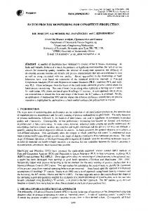
The particular nature of the problem then depends on which of these components is known and which is to be identiÞed. Each type of problem is associated with a name which changes from discipline to discipline. The choice of the names listed below was motivated by the relative spread of the respective term in the communities. The following principle problems are deÞned (Figure 2.1):

Figure 2.1: The three base problems. • Simulation: Given model, given input data and given parameters Þnd the output of the process. • IdentiÞcation: Given model structure, some times several structures, given process input and output data, and a given criterion, Þnd the best structure and the parameters for the parameterised model, where “best” is measured with the criterion. • Optimal Control: Given a plant model, a criterion associated with process input and process output, and the process characteristics, Þnd the best input subject to the criterion. The deÞnition of simulation is straightforward. The task of identiÞcation though is not, in that it includes Þnding structure as well as parameters of a model. This in turn implies that many tasks match this description, such as process design and synthesis, controller design and synthesis, parameter identiÞcation, system identiÞcation, controller tuning and others Þt this definition. The deÞnition of the optimal control task is also wider than one usually would project. Namely process scheduling and planning are part of this deÞnition as well as the design of a shut-down sequence in a sequential control problem, to mention a few non-traditional members of this class. In all three classes a model is involved. In this discussion parameterised input/output mapping are used because they are usually the type of model capturing the behaviour of a given system in the most condensed form. Though in each case it is solved for a different set of its components. In the case of the simulation, the outputs are being computed, in the case of the identiÞcation task, the best parameters are found and in the case of optimal control, the best input record is being determined.

2.2 The Modelling Process

17

In order to solve a problem, the model must be supplemented with a set of deÞnitions, which, in combination with the model, deÞne a mathematical problem that can be solved by a particular mathematical method. These deÞnitions are instantiations of variables that assign known quantities to variables or functions of know quantities, where the functions may be arbitrarily nested. On this highest level, process engineering problem solving has four principle components : 1. Formulation of a model; 2. Problem speciÞcation; 3. Problem solution method; 4. Problem analysis. The following sections discuss the problem of the model formulation in more details.

2.2

The Modelling Process

Models take a central position in all process engineering tasks as they replace the process for the analysis. They represent an abstraction of the process, though not a complete reproduction. Models make it possible to study the behaviour of a process within the domain of common characteristics of the model and the modelled process without affecting the original process. It is thus the common part, the homomorphism or the analogy between the process and model and sometimes also the homomorphism between the different relations (== theories) mapping the process into different models that are of interest. The mapping of the process into a model does not only depend on the chosen theory, but also on the conditions under which the process is being viewed. The mapped characteristics vary thus not only with the applied theory but also with the conditions. Different tasks focus on different characteristics and require different levels of information about these characteristics. For example control would usually be achievable with very simple dynamic models, whilst the design of a reactor often requires very detailed information about this particular part of the process (Aris 1978). The result is not a single, all-encompassing model but a whole family of models. In fact, there is no such thing as a unique and complete model, certainly not from the philosophical point of view nor from a practical, as it simply reßects the unavoidable inability to accumulate complete knowledge about the complex behaviour of a real-world system. More practically and pragmatically a process is viewed as the representation of the

18

Introduction to Modelling

essential aspects of a system, namely as an object, which represents the process in a form useable for the deÞned task. Caution is advised, though, as the term essential is subjective and may vary a great deal with people and application. The term multi-faceted modelling has been coined reßecting the fact that one deals in general with a whole family of models rather than with a single model (Zeigler 1984). Whilst certainly the above motivation is mainly responsible for the multi-faceted approach, solution methods also have use for a family of models as they can beneÞt from increasing the level of details in the model as the solution converges. An integrated environment must support multi-faceted modelling, that is mapping of the process into various process models, each reßecting different characteristics or the same characteristics though with different degree of sophistication and consequent information contents. In order to identify components of the suggested environment, the process of deriving process models is the subject of the next section.

2.3

Formulation of the Model

Establishing a model, as it is used in a particular application, involves a number of operations, which can be broken down into a number of principle steps. Analysing the operations on each individual step then reveals the communalities and differences. The object being mapped is referred to as the plant which is here used as a synonym for physical-chemical-biological system, an entity which transforms matter by the means of a chemical or biological process in a physical environment. Alternative models can be generated in one of two ways. The Þrst approach is to use different theories to map the plant into a mathematical object thus obtain different mathematical models using different theories. The second possibility is to manipulate one of the models deriving new models. Again, an integrated environment should allow for both mechanisms. Any manipulation will in general reduce, or at the best maintain, the information contents of the model with respect to structural complexity. The manipulation can only result in transformed models or simpliÞed models.

2.3.1

Primary Modelling Operation

The very Þrst step in the process of obtaining a model is the mapping of the real-world prototype, the plant, into a mathematical object, here called the primary model. This process is non-trivial because it involves structuring of the process into components and the application of a mapping theory for each component. Since the theories are context dependent, the structuring is tightly

2.3 Formulation of the Model

19

coupled to the theory chosen. The process of breaking the plant down to basic thermodynamic systems determines largely the level of details included in the model. It is consequently also one of the main factors for determining the accuracy of the description the model provides. Chapter 3 gives an idea on how a process can be broken down into smaller parts using only two basic building blocks, namely systems and connections. The resulting interconnected network of capacities is called the physical topology. In chapter 4 the so-called species topology is introduced. This species topology is superimposed on the physical topology and deÞnes which species and what reactions are present in each part of the physical topology. Structuring is one factor determining the complexity of the model. Another factor comes to play when choosing descriptions for the various mechanisms such as extensive quantity transfer and conversion. For example in a distributed system, mass exchange with an adjacent phase may be modelled using a boundary layer theory or alternatively a surface renewal theory, to mention just two of many alternatives. The person modelling the process thus will have to make a choice. Since different theories result in different models, this implies making a choice between different models for the particular component. Structuring and use of theories will always imply intrinsic simplifying assumptions. For example modelling a heat transfer stream between the contents of the jacket and the contents of a stirred tank may be modelled using an overall heat transfer model, that is a pseudo-steady state assumption about the separating wall and the thermal transfer resistant of the ßuids is made. Though, if one is interested in the dynamics of the wall, a simple lumping of the wall improves the description or if this is still not sufficient one may choose to describe the heat transfer using a series of distributed coupled system or a series of coupled lumped systems. Assuming for the moment that the structuring is not causing any problems and assuming that a theory or theories are available for each of the components, the mapping into a mathematical object associated with a chosen view and an associated theory is formal. The presumption is made that no other intrinsic assumptions are being made at this point, that is, the theory is applied in its purest form. SpeciÞcally, the conservation principles, which describe the basic behaviour of plants, are applied in their most basic form. Particularly the energy balance is formulated in terms of total energy and not in any derived state functions. Chapter 5 discusses the mathematical description of process models (the equation topology) and deals with the last three steps of the modelling method (outlined in the Þrst chapter of this thesis), since all of these steps involve equations. This chapter is devoted to ”proper model building”, so assumptions that implicate modelling difficulties are kept clear of.

20

2.3.2

Introduction to Modelling

Assumptions about the Nature of the Process

Once a mathematical model for the process components has been established, usually the next operation is to implement a set of assumptions which eliminate complete terms or parts thereof in the equations of the primary model. These are assumptions about the principle nature of the process such as no reaction, no net kinetic or potential energy gain or loss, no accumulation of kinetic or potential energy. Whilst not complete, this is a very typical set of assumptions applied on this level in the modelling process. The assumptions are of the form of deÞnitions, that is variables, representing the terms to be simpliÞed are instantiated. For example, the production term in the component mass balances might be set to zero. Additional assumptions that simplify the process model may be introduced at any point in time. A very common simpliÞcation is the introduction of a pseudo-steady state assumption for a part of the process which essentially zeroes out accumulation terms and transmutes a differential equation into algebraic relation between variables. These can then be used to simplify the model by substitution and algebraic manipulation. The Þnal chapter of this part, chapter 6, discusses which alterations have to be made to the equation topology when certain assumptions are being made.

Chapter 3

Hierarchical Organisation: The Physical Topology In order to get a mathematical description of a process, a modeller usually has to break the process down into smaller parts for convenience reasons. A process is thus assumed to consist of a set of subprocesses. These subprocesses may in turn be divided into smaller processes, and so on, until the process consists of a number of subprocesses, which each are small enough to be handled individually. In the modelling method that we employ this means that a process is divided into a network of interconnected volume elements. Each volume element of such a network consists of a single phase that is uniformly distributed and hence displays uniform properties over its volume. The network of volume elements describes, so-to-speak, the physical structure of the process and shall be referred to as the physical topology of that process. The physical topology contains, once established, the maximum of information about the dynamic phenomena captured in the model. Any modiÞcation on the topology changes the dynamic information contents.

3.1

Building Blocks

The physical topology is built from only two principle components, namely systems and connections. The systems (volume elements) represent capacitive elements able to store extensive quantities (such as mass, energy and momentum) and are therefore associated with mass. The connections describe the exchange of extensive quantities between two such capacities. Hence, systems and connections appear in an alternating sequence in a process representation. As mentioned before, a process can be decomposed into a set of interactive thermodynamic systems based on classical axiomatic thermodynamics. 21

22

Hierarchical Organisation: The Physical Topology

A thermodynamic system is deÞned (Tisza 1961) as a Þnite region in space speciÞed by a set of physically quantiÞable variables. Such a system consists of a phase. The systems concept, though, does not require uniform conditions within this phase. So, in order to deÞne a consistent and generic primitive modelling component - for the sake of basic and fundamental modelling - we have to slightly adjust this deÞnition. One can distinguish between two ”types” of systems. The Þrst are lumped systems, which have a homogeneous or uniform phase and consequently have uniform intensive properties (such as concentration, temperature and density). The others are distributed systems, which do not exhibit uniform conditions across their phase: the intensive properties are gradually changing with the deÞned spatial coordinates. These two types can be mapped into one by deÞning only one primitive simple system that may be of Þnite or differentially small volume. This results in the following deÞnition: Definition 3.1.1 A simple system (Σ) is a body of Þnite or differentially small volume consisting of a single phase or a pseudo-phase This deÞnition implies that a capacity of any nature is present in the system and that the state of the system is uniform within the spatial domain it occupies. In the deÞnition the system is called a simple system because it relates to a single uniform phase or a pseudo-phase within the system. The phase concept is hereby extended by allowing for a pseudo-phase. This is done in order to support the granularity concept. A pseudo-phase is a spatial domain with spatially averaged properties and is associated with the granularity of the model. On a Þner scale, the phase concept applies usually well, but as one increases the granularity, i.e. larger spatial domains are represented as systems, the systems spatial domain may not exhibit uniform physical properties any more. However, for the purpose of the model, one may still want to view this domain as a uniform system. For this reason the pseudo-phase concept is introduced. A system represents a capacity and is separated from its neigbouring systems by means of an imaginary wall of no mass and therefore of no capacity. This boundary, which encapsulates the total mass of the system, is a theoretical artifact. Although these boundaries often replace physical walls in a model, they are certainly not the same. Mapping a physical wall into a boundary of a thermodynamic system implies that the capacity effect of the wall is neglected and that it is mapped into an abstract thermodynamic wall. If one wishes to model a wall as a capacitive component, this wall should be represented as a system, and thus be associated with a capacity. Systems are interacting through their common boundaries. Classical ther-

3.1 Building Blocks

23

modynamics deÞnes three classes of systems based on the nature of these interactions, namely isolated, closed and open systems. A thermodynamically isolated system has no interaction with its environment. The interaction of a closed system with its environment is limited to the transfer of heat only, without any exchange of matter. A thermodynamically open system can interact with its environment through its boundary transferring both energy and mass. The interactions between systems are represented by the second type of building block used to construct the physical topology, namely the connections. A connection represents an interaction between two capacitive elements c.q. systems. It describes the exchange of extensive quantities across the boundary separating two adjacent systems. Therefore, a connection cannot exist in isolation. In other words, a connection cannot be established prior to the deÞnition of two distinct systems as origin and target of the connection. The implication of this paradigm is that all plant models are closed. No open ends exist. Any source of material, energy, or any extensive quantity for that matter must be modelled and the same applies for any sink. A connection represents a common boundary segment of the connected systems. An arbitrary number of connections may exist between two systems through any of the common boundary elements. The connections, at this stage, do not specify yet the speciÞc details on how and how much is being communicated through them, only the nature of the connections is deÞned. They can either be mass, heat or work connections. Definition 3.1.2 A connection is a directed communication path for the exchange of a speciÞc extensive quantity between two systems through a boundary element, separating the two systems The deÞnition given above implies that connections are directed. This means that the ßow of the extensive quantity through the connection is measured relative to a reference co-ordinate system. This co-ordinate system is deÞned by the origin and the target of the connection (this is graphically depicted as an arrow with a head and a tail). The actual ßow is caused by a difference in the states of the two systems, such as heat ßow by a difference in the temperature and convective ßow by a difference in the pressure. By convention, the sign of the ßow is considered to be positive when the transferred quantity ßows from the origin to the target. Example 3.1: A General Process. Figure 3.1a represents a general open process, embedded in its environment. The process divided into 3 parts, each of which can

24

Hierarchical Organisation: The Physical Topology

Figure 3.1: a. A general open process and its interaction with its environment, b. Possible physical topology of this process. be modelled as simple thermodynamic systems. Each arrow in this drawing represents the transfer of a speciÞc extensive quantity across the boundary of two adjacent systems. The process can be modelled as a closed process if the environment is considered as a simple system. The interactions between the systems and the environment can then be modelled in the same way as the interactions between the individual systems. Figure 3.1b shows a physical topology of the process. As you can see, the physical topology is built from (lumped) capacities, shown as circles, and directed connections, shown as arrows. Each connection has an origin and a target system. The origin and the target deÞne the reference co-ordinate system for the direction of the ßow of extensive quantity between them. So, if the transferred quantity ßows from the target to the origin, this will correspond to a negative ßow from the origin to the target. ¤ Example 3.2 shows a possible division of a process into smaller parts, which results in a possible physical topology of that process. The physical topology consists only of systems and connections between those systems. Example 3.2: A Possible Physical Topology Figure 3.2a shows a schematic representation of a reactor that could be part of a larger plant. The reactor is divided in four parts by three partitions and the contents of the reactor is heated via the surface of the reactor. The actual contents of the reactor and the reaction(s) taking place in it are of no concern at this Þrst stage

3.1 Building Blocks

25

Figure 3.2: a. Schematic representation of an example reactor, b. Possible physical topology for this reactor. of the model construction. Presently, only a physical topology for this reactor shall be constructed. This topology will form the basis for the rest of the modelling process. A possible division of the reactor into simple systems is shown in Þgure 3.2b. The circles and the square represent capacitive volume elements (simple lumped systems), the arrows represent paths for the exchange of extensive quantities (connections). The reactants are fed into the reactor at the top end, represented by the Þrst lump. A source element was introduced here in order to model the inßow. It is important to realise that if the reactor would be modelled within a larger network, the source might be replaced by another physical element. The source system has to be introduced here, because we have to construct closed process models with our modelling methodology. This means that mass must come from somewhere; it cannot just appear. Then the ßuid passes from one lump to another, until it leaves the reactor at the tail end. The products are collected in a sink system, again because mass cannot just disappear. The heat that is added to each lump is represented by a connection from an energy source, which describes the energy transfer. Obviously this physical topology would result in a relatively simple model of the reactor. The model maps the four parts of the reactor into four individual lumped systems or volume elements. It is implied that within one such volume element the physical conditions are spatially uniform. Of course, this is but an approximation of the physical reality. Also, the representation of the heating surface of the reactor as a simple uniform capacity is an approximation. With the equations that describe the transfer of mass and energy

26

Hierarchical Organisation: The Physical Topology and with the mass and energy balances of each system, we can describe the dynamic and/or static behaviour of the process, provided that enough additional information is added. ¤

The two examples illustrate how a physical topology of a process can be constructed with just two building blocks, systems and connections.

3.2

Domains

Connections can be either mass, heat or work connections and therefore a process model can consist of several domains. In this work a domain has the following deÞnition: Definition 3.2.1 A domain is an interconnected network of capacities (i.e. primitive systems), in which all connections are of the same type . As a rule, single systems, i.e. systems without connections, do not belong to any speciÞc domain. An exception to this rule is a system, which has a capacity to store certain species (see chapter 4). Such a system is a (single) mass domain. We distinguish 4 types of domains, namely: mass, heat, work and energy domains. In energy domains all types of connections are considered. A mass domain can hold several species domains, depending on the presence of those species in the systems and connections of the mass domain. Example 3.3: Domains Within a Physical Topology

Figure 3.3: Physical topology of a process consisting of 8 systems, 6 mass connections and 2 heat connections. Consider the physical topology shown in Þgure 3.3. This physical topology consists of 7 systems, 5 mass connections and 2 heat

3.3 Fundamental Time Scale Assumptions

27

connections. There are 2 species present: species A is present in systems 1, 2, 3, 4, 5 and 6 and ßows through all mass connections. Species B is present in the systems 1, 2, 3, 4, 5, 6 and 7 and ßows through the mass connections m1, m3, m4 and m5. We can identify the following domains: • 2 Mass domains: (1, 2, 3, 4, 5, 6, m1, m2, m3, m4, m5) and (7). • 2 Heat domains: (2, 3, h1) and (5, 7, h2).

• 1 Energy domain: (1, 2, 3, 4, 5, 6, 7, m1, m2, m3, m4, m5, h1, h2). • 1 Species domain for species A: (1, 2, 3, 4, 5, 6, m1, m2, m3, m4, m5). • 3 Species domains for species B: (1, 2, m1), (3, 4, 5, 6, m3, m4, m5) and (7). ¤

3.3

Fundamental Time Scale Assumptions

Physical topologies are the abstract representation of the containment of the process in the physical sense. They visualise the principle dynamic contents of the process model and therefore the construction of a physical topology is the most fundamental part of the modelling process. Any changes in the physical topology will substantially affect the structure and contents of the Þnal model. The structuring of the process implements the Þrst set of assumptions in the modelling process. The resulting decomposition is, in general, not unique. However, the resulting model depends strongly on the choice of the decomposition. As a rule: the Þner the decomposition, the more complex will the resulting model be. The decision of deÞning subsystems is largely based on the phase argument, where the phase boundary separates two systems. The second decision criterion utilises the relative size of the capacities and the third argument is based on the relative velocity with which subsystems exchange extensive quantities. Another argument is the location of activities such as reactions. The relative size of the model components, measured in ratios of transfer resistance and capacities, termed time constants, is referred to as ”granularity”. A large granularity describes a system cruder, which implies more simply, than a model with a Þner granular structure. It seems apparent that one usually aims at a relative uniform granularity, as these systems are best balanced and thus

28

Hierarchical Organisation: The Physical Topology

more conveniently solved by numerical methods. Models of different granularity help in analysing the behaviour of the process in different time scales. The Þner the granularity, the more the dynamic details and thus the more of the faster effects are captured in the process description. Since each model is constructed for a speciÞc goal, a process model should reßect the physical reality as accurately as needed. The accuracy of a model intended for numerical simulation, for example, should (in most cases) be higher than the accuracy of a model intended for control design. To illustrate the concepts mentioned above, consider the following example concerning a stirred tank reactor: Example 3.4: Stirred Tank Reactor Figure 3.4a shows a stirred tank reactor, which consists of an inlet and outlet ßow, a mixing element, a heating element and liquid contents. If the model of this tank is to be used for a rough approximation of the concentration of a speciÞc component in the outlet ßow or for the liquid-level control of the tank, a simple model suffices. The easiest way to model this tank is to view it as an ideally stirred tank reactor (ISTR) as shown in Þgure 3.4b. This implies that a number of assumptions have been made regarding the behaviour and properties of the tank. The most important assumption is the assumption that the contents of the tank is ideally mixed and hence displays uniform conditions over its volume. Another assumption can be that heat losses to the environment are negligible.

Figure 3.4: a. Stirred tank reactor; b. Ideally Stirred Tank Reactor (ISTR).

3.3 Fundamental Time Scale Assumptions

29

After making these and maybe some more assumptions, the modeller can write the total mass balance, component mass balances and the energy balance of the reactor. With these equations and some additional information (e.g. kinetics of reaction, physical properties of the contents, geometrical relations, state variable transformations, etc.) the modeller can describe the dynamic and/or static behaviour of the reactor.

Figure 3.5: a. Graphical representation of a possible mixing in a tank; b. Possible decomposition of this process into volume elements for the construction of a mathematical model. If the tank has to be described on a much smaller time-scale and/or the behaviour of the tank has to be described in more detail, then the ISTR model will not suffice. A more accurate description often asks for a more detailed model. In order to get a more detailed description the modeller could, for example, choose to try to describe the mixing process in the tank (see Þgure 3.5a). Figure 3.5b shows a possible division of the contents of the tank into smaller parts. In this drawing a circle represents a volume element which consists of a phase with uniform conditions. Each volume element can thus be viewed as an ISTR. The arrows represent the mass ßows from one volume to another. In order to describe the behaviour of the whole tank, the balances of the fundamental extensive quantities (component mass, energy and work usually suffice) must be established for each volume element. The set of these equations, supplemented with information on the extensive quantity transfer between the volumes and other additional information, will constitute the

30

Hierarchical Organisation: The Physical Topology mathematical description of the dynamic and/or static behaviour of the reactor. The model of the mixing process could, of course, be further extended to get a more accurate description1 . The number of volume elements could for example be increased or one could consider back mixing or ”cross” mixing of the liquid between the various volume elements. The conduction of heat to each volume could also be modelled. One could model a heat ßow from a heating element to each volume, or only to those volume elements which are presumed to be the nearest to the heating element, etc. As one may imagine there are many ways to describe the same process. Each way usually results in a unique mathematical representation of the behaviour of the process, depending on the designers view on and knowledge of the process, on the amount of detail he wishes to employ in the description of the process and, of course, on the application of the model. ¤

When employing the term time scale, we use it in the context of splitting the relative dynamics of a process or a signal (the result of a process) into three parts, namely a central interval where the process or signal shows a dynamic behaviour. This dynamic window is on one side guarded by the part of the process that is too slow to be considered in the dynamic description, thus is assumed constant. On the other side the dynamic window is attaching to the sub-processes that occur so fast that they are abstracted as event - they just occur in an instant. Any process we consider requires these assumptions and it is the choice of the dynamic window that determines largely the Þdelity of the model in terms of imaging the process dynamics.

Figure 3.6: The dynamic window in the time scale. One may argue that one should then simply make the dynamic window as large as probably possible to avoid any problems, which implies an increase 1

In principle, if one increases the complexity of this description, one approaches the type of models that result from approximating distributed models using computational ßuid dynamic packages.

3.3 Fundamental Time Scale Assumptions

31

in complexity. Philosophically all parts of the universe are coupled, but the ultimate model is not achievable. When modelling, a person must thus make choices and place focal points, both in space as well as in time. The purpose for which the model is being generated is thus always controlling the generation of the model (Aris 1978)(Apostel 1960) and the modeller, being the person establishing the model, is well advised to formulate the purpose for which the model is generated as explicit as possible. A window in the time scales must thus be picked with the limits being zero and inÞnity. On the small time scale one will ultimately enter the zone where the granularity of matter and energy comes to bear, which limits the applicability of macroscopic system theory and at the large end, things get quite quickly infeasible as well, if one extends the scales by order of magnitudes. Whilst this may be discouraging, having to make a choice is usually not really imposing any serious constraints, at least not on the large scale. Modelling the movement of tectonic plates or the material exchange in rocks asks certainly for a different time scale than modelling an explosion, for example. There are cases, where one touches the limits of the lower scale, that is, when the particulate nature of matter becomes apparent. In most cases, however, a model is used for a range of applications that usually also deÞne the relevant time-scale window. The dynamics of the process is excited either by external effects, which in general are constraint to a particular time-scale window or by internal dynamics resulting from an initial imbalance or internal transposition of extensive quantity. Again, these dynamics are usually also constraint to a time-scale window. The maximum dynamic window is thus the extremes of the two kinds of windows, that is, the external dynamics and the internal dynamics. A ”good” or ”balanced” model is in balance with its own time scales and the time-scale within which its environment operates. In a balanced model, the scales are adjusted to match the dynamics of the individual parts of the process model. Balancing starts with analysing the dynamics of the excitations acting on the process and the decision on what aspects of the process dynamics are of relevance for the conceived application of the model. What has been deÞned as a system (capacity) before may be converted into a connection later and vice versa as part of the balancing process. This makes it difficult, not to say impossible, to deÞne systems and connections totally hard. The situation clearly calls for a compromise, which, in turn, opens the door for suggesting alternative compromises. There is not a single correct choice and there is certainly room for arguments but also for confusion. Nevertheless a decision must be taken. Initially one is tempted to classify systems based on their unique property of representing capacitive behaviour of volumes, usu-

32

Hierarchical Organisation: The Physical Topology

ally also implying mass. In a second step one may allow for an abstraction of volumes to surfaces, because in some applications it is convenient to also abstract the length scale describing accumulation to occur inside, so-to-speak, or on each side of the surface. For the sake of modelling, some of the deÞned systems within a physical topology can be deÞned as ”non-dynamical systems”, because the dynamics of these systems is either outside the dynamic window, or is not of interest for the model (for example, the source and sink system in example 3.1). The systems can be divided into six ”sub-classes”: • Lumped • Distributed • Source • Sink • Steady State • Composite In this work we primarily use the lumped systems to describe the dynamics of a process. Distributed systems are systems that do not display strictly uniform intensive properties (such as temperature, pressure, composition, density, etc.) within their boundaries. They are a common phenomenon within the modelling community, but, because of their inÞnite order, one often does not like to have them in the model. One way to remedy this is to let the distributed system undergo a model reduction, thereby mapping them from an inÞnite-order into a Þnite-order system. With this it is accepted that the higher frequency properties of the process are not appropriately reßected in the model. The results are models that apply to the intermediate time scale. Source and sink systems represent resource systems, the dynamics of which are not of interest for the model. These systems are usually inÞnitely large and only the intensive properties are deÞned, since the dynamics (which involve the extensive quantities) of these systems are ignored. Another property of source and sink systems is that the values of the deÞned intensive properties can be altered inÞnitely fast. When the dynamics of a system are very fast as compared to the dynamics of its surrounding systems, a pseudo steady-state assumption is made for this system. This means that the dynamics of a steady-state system are ignored (this will be further explained in section 6.4).

3.4 Hierarchical Organisation

33

Composite systems are introduced to address groups of systems, such that large and complex processes can be handled easier. The next section discusses the hierarchical organisation of physical topologies.

3.4

Hierarchical Organisation

A processing plant has a physical structure and this structure is represented by the physical topology of the plants symbolic model. The physical topology is the basic frame of the model. It represents the modellers view of the plants physical structure: It describes the containment of and the interactions between the different internal structural elements. Once constructed it determines the model order and with it an important portion of the dynamics. The physical topology of a processing plant is the foundation for the process information, which is added in the next two stages of the modelling process. The physical topology is constructed by deÞning the components of the processing plant in the form of simple thermodynamic systems, which will eventually describe the physical behavior of a spatial domain, occupied by the plant. At this Þrst stage of the model deÞnition process, though, these physical primitive systems can be seen as container-like items that have not yet been Þlled nor further speciÞed. In the previous examples, the number of primitive components (simple systems) of the physical topology was very small. These processes could easily be represented as a network of primitive systems and connections. For larger and/or more complex process models, this ßat topology would obviously not be very suitable. The number of systems does not need to grow very large before it becomes rather difficult to maintain an overview over the deÞned model of the process. The design, documentation and manipulation of these models would become very hard. Therefore, an abstraction has to be introduced in the form of a hierarchical deÞnition of the model. This additional structure is laid over the ßat topology in such a way that it allows to address groups of components c.q. composite systems. The result is a tree of systems, with the modelled process as the root node. There exist basically two techniques for developing a physical topology of a process, namely the top-down and the bottom-up approach. A modeller, who uses the top-down approach, starts with a simple initial model, which is based on a crude design. This crude model is then reÞned by adding details in several stages. In each stage the resolution of the model is increased by reÞning an element. In the bottom-up approach, combinations of the simple systems deÞne the next level of systems in the hierarchy (namely composite systems) and so forth

34

Hierarchical Organisation: The Physical Topology

until Þnally on the top level the global system is deÞned, which of course represents the model of the process (the model of the process is a thermodynamic universe). This grouping of individual components is arbitrary, but obviously follows a logical scheme associated with physical location and functionality as well as a degree of interaction between the components. When using the bottom-up approach, a modeller focuses on the reuse of existing model parts that have been already designed for other models. Clearly, all parts of a model may not have been deÞned previously. Thus, both methods are often used in the model building process. A good example to illustrate the hierarchical decomposition of a process is a distillation column. Example 3.5: Hierarchical Decomposition of a Distillation Process A distillation column is a multi-staged column where components are separated due to differences in their vapor pressure. A typical distillation column consists of a column with a central feed, a reboiler to supply the necessary energy, and a condenser for removing most of the energy at the top (see Þgure 3.7b). The overhead vapor stream is cooled and completely condensed, and then it ßows into the reßux drum. The liquid from the reßux drum is partly pumped back into the column (to the top tray) and the rest is removed as the distillate product. At the base of the distillation column, the liquid product stream is split into two streams. The bottom product is drawn from the column, whilst the rest is recycled into the heater for evaporation and is returned to the base of the column. The distillation column itself is considered to be composed of a feed tray and two sections, which here consist of three trays each. Figure 3.7 shows a possible way to decompose the distillation process. This will Þnally lead to a ßat topology of the process (Þgure 3.7e), which consists only of thermodynamic simple systems (circles and squares) and connections (arrows). For the construction of the physical topology as represented in Þg 3.7e, the following assumptions have been made: • Each tray is assumed to consist of two homogeneous phases (a liquid phase L and a vapor phase V) and a ’boundary phase’ B, separating the two homogeneous phases. • The condenser and the reboiler can both be decomposed into three lumped systems and a steady-state (boundary) system.

3.4 Hierarchical Organisation

35

Figure 3.7: Possible decomposition of a distillation process, in Þve steps.

36

Hierarchical Organisation: The Physical Topology One lump as a heating/cooling medium and the other two as homogeneous process phases (liquid and vapor phase). • Heat losses from the column to the surroundings are assumed negligible. • The momentum balances for each tray are neglected. The reference co-ordinate systems of the connections are chosen based on the normal ßow direction of the streams. The mass streams connecting the liquid and the vapor phases on each stage are selected in such a way that the lighter components ßows in the positive direction, and the heavier components in the negative direction.

Figure 3.8: Tree structure representation of a typical distillation column It appears natural to group the different systems and form a hierarchical tree for the representation of the column. Figure 3.8 shows such a hierarchical tree for the distillation process. For simplicity, the connections between the simple systems are left out in this Þgure, because only the tree representation of the physical topology shall be illustrated with this example. Also, the feed stream source and the product sinks, as well as the energy source and sink, are left out in this representation. The tree is composed of Þve hierarchical levels. The root of the tree represents the highest hierarchical level, which of course is the

3.4 Hierarchical Organisation

37

complete distillation column. The column is composed of the distillation tower, the reboiler and the condenser. These three components form the next hierarchical level. The distillation tower is again composed of three components, namely a feed tray, and a bottom and top section, which both consist of three trays. The two heat exchangers, the reboiler and the condenser, are considered to consist of one ”tray”. Each tray is assumed to be composed of two simple systems (a liquid phase and a vapor phase) and a steadystate system (representing the phase boundary). The leaves of the tree are simple systems, the other nodes are composite or composed systems. In this analysis a top down point of view was taken. When constructing the tree from bottom up, one could start the description as follows: The liquid and vapor phase, which are both simple systems, are grouped to form a composite system, namely a tray. Trays in turn are grouped to form the bottom and top section of the distillation tower, etc. Either way, the hierarchical structuring of a process will result in a tree of systems, the leaves of which are the thermodynamic simple systems which thus deÞne the physical topology of the process. ¤ Hierarchical grouping of the simple systems will always result in a hierarchical tree of systems with the modelled plant as the root node. The representation of the physical topology of a processing plant in the form of a tree is merely a matter of convenience. The handling of complex systems is supported by hierarchical arrangement of the model components. The hierarchical tree which is superimposed on the basic network, the physical topology, serves as a means to increase the level of abstraction. It increases the efficiency of handling the components and it facilitates the grasping of the essence of the whole process or parts of it (this will be illustrated in chapter 8). The system, however, is completely deÞned on the lowest level, the leaves of the strictly hierarchical multi-way tree, which represent the simple thermodynamic systems. The reÞnement ”multi-way” relates to the fact that each subsystem may divide into an arbitrary number of subsystems. The tree is limited to a ”strictly hierarchical” decomposition, because the conservation principles must hold for any part of the system. This means that none of the elements can be part of two subsystems at the same time; cross links between branches of the tree are thus prohibited. Why the employed tree structure has to be strictly hierarchical can be proved with the following simple proof:

38

Hierarchical Organisation: The Physical Topology

Proof. Proof for strictly hierarchical decomposition (Preisig, 1991c) Let the overall system Σ, which represents the thermodynamic universe, be composed of the two subsystems Σ1 and Σ2 . The system Σ1 in turn consists of the subsystems Σ11 , Σ12 and Σ13 . System Σ2 is composed of Σ13 and Σ21 . Figure 3.9 represents this tree structure. The leaves of the tree, i.e. the systems on the lowest level, which don’t have any subsystems, represent the simple thermodynamic systems. The other nodes represent the composite systems. As illustrated, this tree is not strictly hierarchical because of the cross links between Σ1 and Σ2 to Σ13 .

Figure 3.9: A non-hierarchical tree. Denoting the mass balance of the overall system Σ as MΣ , the following relation exists: MΣ = MΣ1 + MΣ2

(3.1)

correspondingly, the mass balances for Σ1 and Σ2 are as follows: MΣ1 = MΣ11 + MΣ12 + MΣ13

(3.2)

MΣ2 = MΣ13 + MΣ21

(3.3)

substitution of the equations 3.2 and 3.3 in the overall mass balance equation 3.1 results in: MΣ = (MΣ11 + MΣ12 + MΣ13 ) + (MΣ13 + MΣ21 ) = MΣ11 + MΣ12 + 2MΣ13 + MΣ21

(3.4) (3.5)

Thus, the subsystem Σ13 is counted twice, which contradicts the conservation principles.

Chapter 4

Chemical Distribution: The Species Topology Processing plants comprise of various physical, chemical and/or biological processes in which their behaviour depends on the properties and the amounts of the involved mass components. Mass is a carrier of capacity and it forms the body or volume of the systems in the physical structure of the plant. Hence it is essential in the formulation of process models. Knowledge about the involved species and reactions is often required for the behavioural description of a processing plant, because the behaviour of the plant is often species dependent. For example, the dynamics of reactions and the transfer of extensive quantities are characterised by kinetic laws and transfer laws, respectively. These laws, which are usually part of the fundamental models of processing plants, are deÞned as variables and constants, whose values (at least partially) depend on the physical properties of the involved species and the reactions between these species.

4.1

Chemical Distribution

The idea of the construction of the species topology is to facilitate the deÞnition and identiÞcation of species and reactions occurring in various parts of the processing plant. The species topology deÞnes which species are present in which part of the process and thus deÞnes the basics of the chemistry/biology of a processing plant model. This enables the generation of the relevant balances of extensive quantities for the systems. The species topology is superimposed on the physical topology. Its construction efficiently aids the model designer in the deÞnition of the chemistry/biology of the processing plant because it generates knowledge about which species are present in every system in a physical topology and about 39

40

Chemical Distribution: The Species Topology

which reactions occur in every reactive system. It should be noted that at this stage of the model deÞnition process the quantities of the species in the systems are of no relevance. The association of a certain species with a certain system only implies that this system has a capacity for this particular species. If, for example, a system Σ is associated with only one species, S, then this implies that species S is the only species that can be present in system Σ. It does not imply that S has to be present in Σ. At certain moments or maybe all the time during an evolution/simulation of the process, species S may even be absent. At these particular moments the system has no mass, but of course still has a capacity to store the species S. The existence of certain species and reactions in one part of the system does not imply that they are the same in all parts of the system. In principle, however, every chemical or biological species could be present in any part of the system, so one could decide not to construct the species topology and only generate a global set of species. This would mean that one deÞnes only one set of species, which comprises all species that appear in the whole plant. Every primitive system of the physical topology would then consist of all these species. For each species in each system the species mass balances could then be generated, which would of course result in a ßood of equations. In most cases, many of these equations would be obsolete, because species are usually constrained to a group of systems and therefore do not appear in every system. The species of the ßuids in the two parts of a shell and tube heat exchanger, for example, are usually not the same. To aid in the deÞnition of the species topology, species and reaction databases are used and three concepts are introduced, ”permeability”, ”uni-directionality” and ”reactions”, which support the idea of locality of chemical or biological species. These three concepts will facilitate the deÞnition of the species topology and will be illustrated in the next sections. The permeability and uni-directionality concepts are associated with connections and therefore with the common boundary element which the two connected systems have in common.

4.2

Permeability of Mass Connections

The permeability is deÞned as a property of a mass connection, which constrains the mass exchange between systems by making the species transfer selective. The mass connection is then deÞned as a semi-permeable thermodynamic wall. An example of a process where the permeability concept could come in handy is a simple diffusion process. The application of the selective

4.2 Permeability of Mass Connections

41

constraint on the transportation of species can also assist in the representation of separation processes, such as ultra-Þltration or reverse osmosis. Example 4.1: Diffusion of a Component from one Phase to Another

Figure 4.1: a. A tank with two immiscible phases, b. Possible ßat topology of diffusion process. Consider a tank which contains two immiscible phases A and B (Þgure 4.1a.) Phase A consists of species P and Q. Phase B consists of species P and R. The simplest way to describe the diffusion of species P from phase A to phase B (or the other way around) is shown in Þgure 4.1b, which represents a ßat topology of the diffusion process. The two phases are each modelled as a simple lumped system and between the systems exists a mass connection which describes the transfer of all species between those systems. Remember that the direction of the connection is only a convention, deÞning a reference direction for the actual stream. The actual direction of the ßow depends on the driving force, which in this case would be the difference in chemical potentials of P in each phase. To prevent the species Q and R from being transferred through the connection, the permeability concept is introduced: The connection between the two systems is deÞned as a semi-permeable thermodynamic wall, which is only permeable for species P . This means that only the species P will be transferred through the connection and that, consequently, the transfer terms of the other species (Q and R) will not appear in the (component) mass balances of the systems because they are not transferred. ¤

42

Chemical Distribution: The Species Topology

Note that in principle the permeability concept does not have to be limited to mass c.q. species. The concept can be readily extended to any extensive quantity. In practice, though, this is not necessary as one normally distinguishes between mass, heat, momentum and work transfer, which are all handled individually (Preisig et al. 1990), (Preisig et al. 1989).

4.3

Uni-directionality of Mass Connections

The concept of uni-directionality is also a property that is related with mass connections. The species topology, as it was described so far, allows for bidirectional ßow in any mass connection. Since the ßow is (normally) dependent on the state of the two connected systems, nothing can be said a priori about the direction of the actual ßow. In fact, in many situations the ßow would change in the course of the time interval over which the process is being observed. Species that are not inhibited by a deÞned permeability may thus appear on both sides of the connection, when computing the species topology. In many applications, though, one-directional ßows are assumed and thus species propagate in a constraint ßow pattern across the network. This desired behaviour calls for deÞning two classes of mass connections, namely uni-directional and bi-directional, where the latter should be the normal case as it leaves the system unconstraint. Inversion of the ßow for a uni-directional ßow would have to be handled as an exception as it contradicts the validity range of the model.

4.4

Reactions

The reaction concept more or less speaks for itself. A chemical or biological reaction is a mechanism that transforms a set of species, the reactants, into a set of different species, the products. At this stage of deÞning the species topology it is only necessary to know which species are transformed and which species are generated in every (reactive) thermodynamic system. The properties of reactions (kinetic laws, heat of reaction, etc.) and the conditions under which the reaction may take place are introduced at a later stage.

Chapter 5

Mathematical Description: The Equation Topology Having completed the Þrst two stages of the modelling process, it is already possible to generate the dynamic part of the process model, namely the (component) mass and energy balances for all the elementary systems, using the conservation principles (Westerweele 1999). The resulting (differential) equations consist of ßow rates and productions rates, which are not further speciÞed at this point. In order to fully describe the behaviour of the process, all the necessary remaining information (i.e. the mechanistic details) has to be added to the symbolic model of the process. So, in addition to the balance equations, other relationships (i.e. algebraic equations) are needed to express transport rates for mass, heat and momentum, reaction rates, thermodynamic equilibria, deÞnition of intensive variables, and so on. The resulting set of differential and algebraic equations (DAEs) is called the equation topology. From a certain point of view the modelling process can thus be regarded as a succession of equation-picking and equation-manipulation operations. The modeller has, virtually at least, a knowledge base containing parameterised equations that may be chosen at certain stages in the modelling process, appropriately actualised and included in the model. The knowledge base is, in most cases, simply the physical knowledge of the modeller, or might be a reßection of some of his beliefs about the behaviour of the physical process. In this chapter a classiÞcation of the variables and equations that are occurring when modelling physical/chemical systems is made. Next, a concise, abstract canonical form is presented, which can represent the dynamics of any physical-chemical-biological process. After that, the algebraic equations, that are necessary to complete the mathematical model of the process, are classiÞed. The proposed classiÞcations make modelling into an almost trivial activity. A link to linear system and control theory is given by transforming the model 43

44

Mathematical Description: The Equation Topology

representation such that is resembles a linear state space description. At the end of the chapter substitutions and variable transformations are criticised and control is brießy discussed.

5.1

Variable ClassiÞcation

The conservation of extensive quantities forms the foundation for describing the dynamic behaviour of systems. Therefore, the set of conserved quantities are called fundamental extensive quantities or the primary state. In section 5.3 it will be shown that the dynamic part (i.e. the differential equations) of physical-chemical-biological processes can be represented in a concise, abstract canonical form, which can be isolated from the static part (i.e. the algebraic equations). This canonical form, which is the smallest representation possible, incorporates very visibly the structure of the process model as it was deÞned by the person who modelled the process (Westerweele and Preisig 2000): The system decomposition (physical topology) and the species distribution (species topology) are very visible in the model deÞnition. The transport and production rates always appear linearly in the balance equations, when presented in this form: x= ú Az + Br in which x :: z :: r ::

(5.1)

Fundamental state vector Flow of extensive quantities Kinetics of extensive quantity conversion

The purpose of the following classiÞcation is to provide a more effective link between thermodynamics and system theory. The classiÞcation of variables that is presented here is, in the Þrst place, based on the structural elements of the modelling approach (namely systems and connections). The subclassiÞcation has its origins in thermodynamics. The variables that appear in the mathematical model of a process are divided into three main groups, namely system variables, connection variables and reaction variables.

5.1.1

System Variables

System variables are variables that are deÞned within the boundary of a system (or sometimes a group of systems). They can be subdivided into two main groups: • The basic type of variables are the fundamental extensive variables or fundamental state variables (x) representing the quantities for which

5.1 Variable ClassiÞcation

45

conservation laws are valid and for which we write balance equations (See section 5.2). In most chemical processes, these are component masses (total mass is the sum of the component masses), energy, and momentum. • The second group of variables is called application variables or secondary state variables (y), which is a gathering of two categories, intensive and geometrical variables, as well as other variables not covered by the previous classiÞcation. The secondary state variables are quantities that are derived from the primary state (x). The secondary state must be the result of a mapping of the primary state (y=f (x)). Thus in any model, this link must exist. Intensive variables are those that provide a local characterisation of the process. We distinguish among them potentials that are driving forces for ßows such as temperature, pressure, chemical potential, and physical properties characterising the “quality” of the material such as density, or concentration. Geometrical variables are those that characterise the dimension conÞguration of the process, independent of the presence of the physical process. They may describe the extent of the process such as volume, area, etc. or give localised characteristics such as porosity, tortuosity, etc. The choice of the intensive and geometric variables that characterise the process is very much application dependent in the sense that it is determined by the Þnal goal of the model. A common property of the intensive and geometric variables is that, in general, these are the variables for which direct information through measurements is available.

5.1.2

Connection Variables

Connection variables are associated with physical connections and can be divided into two groups: • Flow rates of fundamental extensive quantities represent the rates by which the respective quantities are exchanged between two interconnected elementary systems. An important aspect that we retain for our analysis is that some transfers may induce ßows of several fundamental extensive quantities. For example, a mass transfer will induce ßows of component masses for each substance present in the transferred material, but also ßows of momentum and energy. Similarly, a momentum transfer induces also an energy transfer in the form of mechanical work. In general, each physical connection has assigned a unique fundamental ßow and, possibly, several (or no) induced ßows.

46

Mathematical Description: The Equation Topology We distinguish in our model between fundamental or primary ßow variables (z) and secondary ßow variables. The primary ßow variables are the variables that appear directly in the balance equations. Secondary ßow variables are related to the primary ßow variables via an algebraic expression and do not appear in the balance equations (when, of course, no substitutions have been made). For example, the mass ßow rate (primary ßow variable) of a mass stream of incompressible ßuid can be easily expressed as a function of the corresponding volumetric ßow (secondary ßow variable). The ßow rates are usually deÞned as a function of the secondary state variables of the two interconnected systems (z=h(yor , ytar )). The variables that represent ßow rates will be marked by a hat “ˆ”. For example, m ˆ will typically denote a mass ßow. • Application variables are a gathering of physical properties, geometrical variables and other variables that are related to the connection (i.e. the common boundary of the two interconnected systems).

5.1.3

Reaction Variables

The last group, the reaction variables, will also be split up into two subgroups: • Production rates (r) of fundamental extensive quantities represent the rates by which the respective quantities are produced inside an elementary system. The typical example are the chemical reaction kinetic rates. These variables are associated with those phenomena in which transformations of fundamental extensive quantities occur inside an elementary system. Such is the case for chemical reactions in which component masses are being transformed into one another. As in the case of ßow rates, we can speak of fundamental production rates and induced production rates. In the case of chemical reactions, it is common practice (see (Aris 1969)) to use the extent rate of a reaction to describe the evolution of the reaction. The consumption rates of reactants and the production rates of the reaction products are expressed in terms of the extent rate of the reaction and thus become induced production rates. The production rates are usually deÞned as a function the secondary state variables of a system (r=g(y)). The variables that represent production rates will be marked by a tilde “˜”. • Application variables are a gathering of variables that are related to the reaction (for example, the pre-exponential kinetic constant or the activation energy of a reaction).

5.2 Fundamental State Variables and Equations

5.2

47

Fundamental State Variables and Equations

The behaviour of a system is characterised by the evolution of its state with time. The choice of the elementary system is driven by the choice of the timescale in which the dynamics of the system is to be resolved. This choice is fundamental to the analysis. In order to characterise the behaviour of a system, information is needed about the natural state of this system (at a given time) and about the change of this state with time. The natural state of a system can be described by the values of a set of fundamental extensive quantities, while the change of state is given by the balance equations of those fundamental variables. The fundamental extensive variables represent the ”extent” of the system c.q. the quantities being conserved in the system. In other words: they represent quantities for which the conservation principle and consequently also the superposition principle applies. So, for these variables, the balance equations are valid. In most chemical processes, the fundamental variables are: component mass, total energy and momentum. But other extensive quantities (charge, for example) might be necessary sometimes and will obviously have to be present in a generic modelling tool. The dynamic behaviour of a system can be modelled by applying the conservation principles to the fundamental extensive quantities of the system. The principle of conservation of any extensive quantity x of a system s states that what gets transferred into the system must either leave again or is transformed into another extensive quantity or must accumulate in the system (In other words: no extensive quantity is lost). Symbolically we can write a balance equation for the fundamental extensive variable xf that characterises the elementary system s as: X d f X xs = αc x ˆc + x ˜p (5.2) dt c p where the Þrst sum is taken over all the physical connections c which contribute to the exchange of xfs and the second sum is taken over all production/consumption processes p. Further, x ˆc represents the corresponding ßow rate of extensive quantity x through connection c and x ˜p corresponds to the production rate (which is assumed to be of negative sign if it corresponds to a consumption process). The direction of the ßow through a connection is deÞned relative to the reference co-ordinate system, which, in essence, is introduced for the consistency of the models. This means that a ßow is positive if it moves in the reference direction and negative when it moves in the opposite direction. Adding the predicate of direction to every ßow allows for dynamic changes of the directionality without affecting the structure of the involved equations. Further,

48

Mathematical Description: The Equation Topology

the transfer is deÞned only once and is then incorporated in the two sets of balance equations describing the behaviour of the two connected systems. The coefficients αc ∈ {−1, 1} indicate the conventional direction of the ßow rate x ˆc .

5.3

Balance Equations

This section focuses on the representation of the dynamic part of process models with the aim to generate a minimal representation, which, though, still shows clearly the structural elements for further use. This allows us to separate the consecutive operations, such as model reduction and implementing various assumptions, clearly from the development of the primary model. Another important application of identifying structures in the modelling process, is to use the extra available information to perform efficient model manipulations in order to achieve, for example, superior numerical performance. Ideas to use model structure for DAE index reduction, for example, can be found in (Marquardt 1995), (Moe 1995) and (Westerweele and Preisig 2000). Whilst we consider this approach elementary, the suggested approach is clearly new. We present a new concise, abstract canonical form, which is able to represent a very wide range of dynamic equations of Þrst-principle process models, including physical, chemical and biological processes (Westerweele 2001). We call it canonical because it is minimal whilst, at the same time, showing all the structural elements of the process models clearly: the physical topology and the species topology, both of which were deÞned in the preceding chapters.

5.3.1

Mass Balances

Mass is one of the prime extensive quantities when modelling physical-chemical processes. The generic balance equation (5.2) applies to any of the species present in the system, whereby the number of independent balances is equal to the number of species, that is, if no constraining assumptions are being made. The total mass balance is always the sum of the component balances, thus it is linearly dependent on the component masses. In most applications it is convenient to use the component mass balances as the basic set of equations. The accumulation of the component masses in a system (Σ) is balanced by the transfer across the system boundary and the internal conversion through reactions: X αm n ˆm + n ˜Σ (5.3) nú Σ = ∀m

5.3 Balance Equations where nΣ n ˆi αi n ˜Σ

:: :: :: ::

49

Vector of species, in moles Molar massßow of mass connection i Unit direction of reference co-ordinate ∈ {−1, 1} Production rate for all species

This equation represents the component mass balances of any dynamic system, which is deÞned in a model of a physical-chemical process. We are interested in Þnding a concise, abstract general form which represents the complete model of any physical-chemical process. In the following subsections the balance equations (5.3) will be rewritten with the aim of Þnding a general form for the representation of an interconnected network of systems. Matrix Notation for Production Term The production term n ˜, which appears in the component mass balance for a particular species Aj of an elementary system Σ, includes the information about the rate of consumption or production of this species. This production term is therefore deÞned as the sum of the rate expressions of each elementary reaction, which involves the species Aj . Kinetic rate equations or ”reaction laws” are empirical relations, which describe the rate of conversion of one species (Aj ) in an elementary reaction as a function of the concentration of all the species in the system. The empirical relations are very often power laws, with the exponents reßecting the number of molecules of that particular species involved in the reaction. Chemical reactions are deÞned as stoichiometric equations that relate a number of reactant molecules with a number of product molecules: |ν 1 |A1 + |ν 2 |A2 + ...... À ......... + |ν n−1 |An−1 + |ν n |An With νi Ai

:: ::

Stoichiometric coefficient ith species

(5.4)

(>0 for products, l) ”unknown” quantities can be computed with the remaining equations. The unknown quantities of the steady-state system are now effectively calculated via the imposed constraints. Note 2: In this case, the same results would have been obtained when the systems 1 and 3 would have been connected via a single connection (with system 2 not being present). If a fast ßow assumption would be made (e.g. cA,1 = kcA,3 ), mathematically the same model would result. The former case is, however, more general and can be easily extended to multiple connections. ¤

6.5

Events and Discontinuities

In this work, the dynamic behaviour of a process is abstracted to the point at which it can be represented by the smooth, continuous change of a series of state variables. This allows such a process to be represented mathematically as a set of DAEs. The majority of processes, however, cannot be considered entirely continuous, but also experience signiÞcant discrete changes or discontinuities superimposed on their predominantly continuous behaviour (Barton 1992). Such discrete changes, often referred to as events, can either be planned changes, called time events (for example, planned operational changes, such as start-up and shut-down, feed stock and/or product changes, process maintenance, switching a valve) or non-planned changes, called state events (overßow of a tank, (dis)appearance of a phase, inversion of a ßow). The exact time of occurrence of time events is either known a priori or it can be computed from the occurrence of a previous event. The time of occurrence of state events is not known in advance because it depends on the system fulÞlling certain state conditions. In addition to the two types of events we can classify events in an other way, namely in events that do not change the (dynamic) model structure and events that change the (dynamic) model structure. With events that do not change the model structure, the balance equations are not altered, but some algebraic equations are changed. This usually results in a non-smooth continuation of the primary state variables.

6.5 Events and Discontinuities

95

Example 6.7: Tank with Fast and Equilibrium Reaction Consider a tank with an inlet (consisting of two components A and B) and an outlet. The contents of the tank consist of four components (A, B, C and D) among which two fast reactions occur, namely: A+B → C

A À D

(6.56) (6.57)

The Þrst reaction (6.56) is a very fast, one way reaction. This means that there is no measurable inverse reaction and one of the two components A or B will always be completely consumed (i.e.: nA = 0 or nB = 0). The other reaction (6.57) is an equilibrium reaction, which means that there will always be a certain ratio between components A and D (cA = k ∗ cD ). Because both reactions are fast in the context of the viewed time scale, the reaction terms that appear in the balance equations can be removed be using the Simple Index Reduction Algorithm.

Figure 6.3: Simulation of a tank in which a fast and an equilibrium reaction take place. Figure 6.3 shows the result of a simulation of the tank. In this Þgure we can see three events taking place. At the start of the

96

Assumptions: Problems and Solutions simulation there is an excess of A in the tank, which means that there will be no B, since all B that is available directly reacts with A to form C. The inlet ßow contains more B than A and this results in diminishing quantities of A (and, consequently, D) in the tank until the amount of A (and D) in the tank reaches zero. At this point we encounter the Þrst event, for now there will be an excess of B available in the tank and A (and D) will be non-existent. At a certain point in time the input is changed such that the inlet ßow will contain more A than B. A second event is the result. The amount of B will decrease until is reaches zero. This will initiate the third event, such that A (and D) will be present again. Obviously, the Þrst and last event were state events, while the second event was a time event. ¤

With events that change the (dynamic) structure of the model, not only algebraic equations are altered, but also (parts of) the dynamic balance equations, because the events trigger certain index problems. This means that the number of differential variables will increase or decrease after the event has occurred. Examples of these events are a tank that suddenly overßows (when the overßow is modelled with a constraint (constant volume of the contents), the number of differential variables will have to decrease, due to the introduced index problem), a suddenly starting (or stopping) equilibrium reaction or a system that runs empty. This type of events can cause jumps in the primary state variables, although it usually does not. Example 6.8: Tank of Small Diameter This example shows what kind of problems may arise when a system is discretised into a set of interconnected subsystems.The physical topology of a tank with a small diameter is considered to consist of four interconnected systems, each with a maximum volume of Vmax . The volumetric outlet ßow (Vˆ5 ) is a function of the height (c.q. the pressure) of the liquid in the tank. The height is a ”composite” quantity because it is derived from the sum of volumes of the four systems. If the tank is almost full (i.e. VII = VIII = VIV = Vmax ), the ßow rate through connection 2 can be calculated by making the ”assumption”: VII = Vmax , and subsequently applying the Full Index Reduction Method. Similarly the ßows of connections 3 and 4 can be calculated. (The result will, of course, be that all these ßows are equal to the outlet ßow if constant density is assumed).

6.5 Events and Discontinuities

97

Figure 6.4: A tank with small diameter and a possible physical topology. A problem arises when system I becomes completely empty. The assumption that VII = Vmax is no longer valid, because VII < Vmax and VI = 0. The liquid no longer accumulates in system I and the states of system I become obsolete. The ßow through connection 2 will now be calculated by making a steady-state assumption over system I. (The result will be that the ßow through connection 2 equals the ßow through connection 1). This event will remove the states of system one and also the Full Index Reduction on system II will have to be ”undone”, because connection 2 no longer constrains this system. The mathematical description for connection 2 will be as follows:  VI > 0 : VII = Vmax    (calcutate n ˆ2 via Full Index Reduction) n ˆ2 : = 0 : n ú = 0 V  I   I (calculate n ˆ 2 via Steady-State Assumption) Clearly, the dynamic structure of the model changes when the event occurs. The handling of events that change the dynamic structure of the model by (numeric) solvers is far from trivial and goes beyond the scope of this thesis.

¤ Whatever type of event, there will always be some kind of discontinuity or ”non-smoothness” in the DAE. To solve DAEs with discontinuities successfully, the time integration has to be stopped at the discontinuity and restarted

98

Assumptions: Problems and Solutions

with new consistent initial conditions (Majer and Gilles 1995). These consistent initial conditions can usually be quite easily found from the conditions of the process just before the event occurred. In many cases (especially when the dynamic model structure is not altered) the ”new” initial conditions are actually the same as the conditions just before the event and it will often not be necessary to stop and restart the time integration.

6.6

Variables and Algebraic Equations for Composite Systems

Sometimes it is convienient, or even necessary, to introduce variables and algebraic equations for composite systems. In the last example of the previous section a ”composite” quantity was, for example, introduced to describe the height of the liquid in the tank. In this case this height was used to calculate the magnitude of the outlet ßow. Composite variables are deÞned via algebraic relations as a function of the variables of the subsystems. In the case of extensive quantities, the composite variable will, obviously, be the sum of these quantities of the subsystems, since the physical topology is deÞned as a strictly hierarchical multiway tree. When the composite variables are just deÞned and used, no mathematical problems will arise, since the new variables are deÞned using already deÞned variables. When, however, a composite variable is constraint (for example: the assumption that the volume of a composite system is constant), mathematical problems could arise. Two cases can be distinguished: • All used variables of the subsystems are directly or indirectly related to their primary state variables and the composite variable holds a constraint. In this case an index problem arises, which will have to be dealt with using either the Simple or the Full Index Reduction Method. As with other high-index cases, there has to be an unmodelled ßow (or reaction) which makes the application of the index reduction method possible. • The composite variable is used to calculate a variable of one of the subsystems. When the composite variable is constraint and all but one of the used variables is properly deÞned in the subsystems, then the composite equation can be used to calculate the remaining variable. Consider, for example, a tank in which a liquid and a gas phase are present and which has an inlet and an outlet ßow. The volume V of the tank is Þxed. The volume of the liquid VL can be calculated from the liquid mass. The remainder part of the tank that is not occupied with liquid is the volume that is occupied by the gas phase (VG = V − VL ). In these special

6.7 Summary and Conclusions

99

cases, a variable of a subsystem is calculated using state information of other subsystems. This solution will not result in an index problem, but the computational causality (this subject is discussed in more detail in section 10.3) of the involved variables and equations should be carefully considered in these cases. Note: Strictly speaking we are not talking about a simulation problem in these cases, since the calculated variable (VG in our example) of the subsystem is not directly related to the primary state variables (the mass of the gas phase). The deÞnition mG = ρG VG could, in this case be used to ”identify” the density ρG (parameter identiÞcation).

6.7

Summary and Conclusions

This chapter showed that assumptions that ”simplify” the process description very often lead to computational difficulties. Luckily, since the assumptions are usually introduced locally, the imposed problems stay local and can also be solved locally. The following list summarises the assumptions a model designer can make during the development of a process model: • Unmodelled ßow ⇒ High index process model. Solutions: — Introduce a constraint that directly or indirectly inßuences primary state variables and apply the Simple Index Reduction Method. Result: The unmodelled ßow is removed from the model description by making linear combinations of the balance equations. The index and dimension of the model will decrease. — Introduce a constraint equation and apply the Full Index Reduction Method. Result: The index and dimension of the model have decreased because some states have been removed and the ßow is calculated from ”new” equations, which are generated from combining some balance equations with differentiated algebraic equations. — Apply a steady-state assumption to one of the connected systems. Result: The dimension of the model is reduced because the states of the steady state system have been removed and the ßow is calculated via the balance equations of the steady state system.

100

Assumptions: Problems and Solutions

• Unmodelled reaction ⇒ High index process model. Solutions:

— Introduce a constraint that directly or indirectly inßuences primary state variables and apply the Simple Index Reduction Method. Result: The unmodelled reaction is removed from the model description by making linear combinations of the balance equations. The index and dimension of the model will decrease. — Introduce a constraint equation and apply the Full Index Reduction Method. Result: The index and dimension of the model have decreased because some states have been removed and the reaction is calculated from ”new” equations, which are generated from combining some balance equations with differentiated algebraic equations. (-) Apply a steady-state assumption to the system in which the reaction is taking place. Result: The dimension of the model is reduced because the states of the steady state system have been removed and the reaction is calculated via the balance equations of the steady state system. Note: This is in general not possible, because usually the number of removed states is larger than the number of unmodelled reactions that have to be calculated. The assumption must therefore be partially used to calculate some other unmodelled quantities and this is most of the time not trivial. • Steady-state assumption ⇒ Reduces the dimension of the model.

A number of unmodelled quantities (either ßows, reactions or secondary state variables) equal to the number of removed states have to be calculated from the steady-state balance equations.

A major advantage of this classiÞcation of assumptions is that it is very easy to do the book keeping. An automatic documentation of all assumptions that are made during the model development is the result. All assumptions become very easily retractable and changeable. In all cases, the introduction of a ”simpliÞcation” leads to a reduction of the dimension of the original model and therefore to a model reduction. Many simpliÞcations are solved by an index reduction which leads to a model reduction. Index reduction and model reduction are, however, not the same thing. The purpose of an index reduction is to transform the model such that a model results that can be solved by problem solving software. The goal of

6.7 Summary and Conclusions

101

model reduction is to simplify the model description such that a (much) faster and simpler code is formed that still represents the actual process behaviour with acceptable accuracy. So, although index reduction is a model reduction method, model reduction is certainly more than just index reduction. This work was not concerned with model reduction, but with the construction of consistent dynamic process models.

102

Assumptions: Problems and Solutions

Part II

Implementation

103

Chapter 7

Introduction to Implementation Solving process engineering without the help of computer-based tools is for almost any problem an unthinkable proposition. Process simulation, process design, controller design, controller testing, data acquisition and model identiÞcation, parameter Þtting, valve and pump selection, column sizing are just a few examples taken from a very large catalogue of chemical plant related operations that are almost exclusively done with computer-based tools. Considering the fact that multiple solutions to individual problems are available from different sources such as software houses or supplier companies, the catalogue of tools is rather large. A process engineer, who is more and more involved in the integrated design of processing plants, is thus faced with a multitude of different software tools, which he uses more or less frequently depending on his allocation. Since each of these packages has been developed in isolation, each has a different interface and applies to different problems though the tools may be used to solve problems associated with the same plant. Often the software is very complex and needs a specialist to deÞne and run problems. Data transfer between tools is not standardised and requires special arrangements or add-on’s. All features which do not enhance team work and productivity. The key to improving efficiency is an increased use of common process information and effictive exchange of data, models and information between the applications. During my research period I have developed a computer tool, called the Modeller, based on the ideas and concepts which are described in the previous chapters. The Modeller is a computer-aided modelling tool to interactively deÞne and modify process models. It aims to effectively assist in the develop105

106

Introduction to Implementation

ment of these process models and facilitate hierarchical modelling of process plants through a user friendly interface. The Modeller constructs the process models from primitive building blocks, being simple thermodynamic systems and connections, as discussed in section 3.1. It does not, in distinction to existing ßow sheeting packages, build on unit models. The Modeller generates symbolic models in the form of differentialalgebraic equations consisting of component mass and energy balances, augmented with transfer laws, physical and geometrical property relations and kinetic laws. In this part the implementation of the modelling method in the computer-aided modelling tool the Modeller is discussed. This part starts with describing the construction and manipulation of physical topologies (chapter 8) for PCB processes with the aid of the Modeller. A special graphical user interface has been developed (and implemented) to handle physical topologies of arbitrary complexity. With the modelling tool, the physical topology of a process can be built using two main operations, namely reÞning an existing system (the top-down approach) or grouping systems (the bottom-up approach). The next chapter discusses how one can construct and manipulate the species topology of a physical topology, using the Modeller. The deÞnition of the species topology is initialised by assigning sets of species and reactions to some elementary systems. To aid in this deÞnition, species and reaction databases are used. The user may also specify the permeability (i.e. selective transfer of species) of individual mass transfer connections. The distribution of the species over all systems is automated and uses the facts that assigned species can propagate through permeable mass connections and species may generate ”new” species (via reactions), which in turn may propagate and initiate further reactions. Finally, the implementation and handling of variables and equations, which constitute the generated models, is discussed. With the information on the physical and species topology Modeller can automatically generate balances of fundamental extensive quantities (component mass, energy and momentum) of every elementary system. In order to fully describe the behaviour of the process, the ßow rates and production rates involved in the balance equations need to be speciÞed. So, in addition to the balance equations other relationships are needed to express thermodynamic equilibria, reaction rates, transport rates for heat, mass, momentum, and so on. A model designer can select a particular relationship from a set of alternatives and connect the selected relationship to a balance equation or to another deÞned relationship. In this way, each term in a balance equation can be expanded by deÞning it as a function of some quantities, which in turn may be expanded again and again. The resulting set of equations (the output of the modelling tool) forms

7.1 Implementation Details

107

a mathematical representation for the behaviour of the process in a speciÞc form, which could serve as an input for problem solving tools.

7.1

Implementation Details

This part, Implementation, mainly describes how the implementation works and not how it was implemented. Although the actual implementation required a lot of work and was far from trivial, I do not consider the implementation details to be an important contribution to this thesis. Elaborating on these details would certainly not aid in the overall understanding of the modelling methodology and its implementation for most of the readers. I do wish to mention something on the actual implementation and especially on some of the low-level modules I have written, since these form the basis for the entire program. The software tool, the Modeller, was implemented using the BlackBox Component Builder 1.4 (http://www.oberon.ch). The BlackBox Component Builder is an integrated development environment optimised for componentbased software development. It consists of development tools, a library of reusable components, a framework that simpliÞes the development of robust custom components and applications, and a run-time environment for components. In BlackBox, the development of applications and their components is done in Component Pascal. This language is a descendant of Pascal, Modula-2, and Oberon (PÞster and Szyperski 1994). It provides modern features such as objects, full type safety, components (in the form of modules), dynamic linking of components, and garbage collection. The entire BlackBox Component Builder is written in Component Pascal: all library components, all development tools including the Component Pascal compiler, and even the low-level run-time system with its garbage collector. In spite of its power, Component Pascal is a small language that is easy to learn and easy to teach. When building or manipulating process models, the construction and manipulation of an earlier step has great inßuence on the construction and composition of the later steps. Manipulating later steps will have no inßuence on the composition of earlier steps and will therefore not alter the entered information of these steps. In implementation terms this means that an earlier step should not know about later steps. So, a tool which constructs only a physical topology should have no knowledge of species, variables or equations. A tool which implements the construction of a species topology must have knowledge about the physical topology but not of variables and equations.

108

Introduction to Implementation

When the different steps are implemented in different components, actions taken on one speciÞc step can be clearly separated from actions taken on another step. A clear separation of the different modelling steps can make operations such as error detection and implementation of new procedures in speciÞc steps a lot less time consuming. The program, the Modeller, is build from several modules, which all handle certain aspects of the implementation The main modules of the program are very applicably called CamPhysTops, CamSpecTops and CamEqTops. On top of these modules other modules are implemented, which handle the graphical user interface (GUI), graphical representation, man-machine interaction, etc. To form a Þrm basis on which the entire program could be build, a few general purpose, low-level modules were written. The two most important of these general purpose modules were named CamTools and CamLists. The module CamTools forms the foundation for undoable and redoable operations. This module uses the implementation of the original BlackBox undo/redo mechanism in such a way that more than one operation can be undone or redone within one call. Appendix A gives the interface deÞnition of the module CamTools and explains how the undo/redo mechanism works. The module CamLists deÞnes the data types List and ListReader, which can be used to handle all kinds of operations that involve lists. Any storable object can be added to a list. All manipulations to a list (adding and removing objects) which alter the contents of the list are implemented as operations. This means that all manipulation actions are undoable (and redoable). Module CamPhysTops deÞnes all the basic tools and operations that are needed to construct physical topologies. The module deÞnes the types System and Connection, which are the two primitive building blocks for the construction of physical topologies. Type PhysTop represents physical topologies, consisting of systems and connections. It provides all the operations and procedures needed to construct physical topologies. A physical topology can be extended by laying, for example, a species topology or a variable topology on top of this physical topology. Also, different graphical representations of the same physical topology could be implemented. Type Extension implements the procedure HandleModification which handles all the modiÞcations made to the physical topology. An extension of the physical topology may implement this procedure to react to changes made in the physical topology. For example, a graphical representation (or a species topology) has to update its data when a system is added or removed. An extension can associate an attribute with every system and every connection of the physical topology. In this way, information of an extension that belongs to a speciÞc system (or connection) is carried by this system (or connection).

7.1 Implementation Details

109

An attribute carries speciÞc information of a speciÞc system or connection. This information should, of course, be related to the extension to which the attribute belongs. A graphical attribute (related to a graphical extension) of a system, for example, could contain information on the location of this system on the screen. Every system and every connection can only contain one attribute of a speciÞc extension. This means that every extension can deÞne two attributes: one for systems and one for connections. The graphical user-interface of the Modeller only contains two main elements. These are the model windows in which the physical topologies of the different models can be constructed and a properties toolbox, which displays the properties and information of the selected object(s) or of the entire model (when no selection is made). The properties toolbox is fully context dependent, which means that if the selection is changed, the properties toolbox will immediately addapt and show the properties of the new selection. In this way it is always clear on which object(s) certain actions are performed.

110

Introduction to Implementation

Chapter 8

Construction of the Physical Topology The construction and manipulation of the physical topology in an easy and fast manner, without compromising on the consistency of the process models, is one of the primary objectives of the computer-aided modelling tool Modeller. The tool should therefore allow for any structural change in any order. In this section the basic operations one can perform on a physical topology are discussed.

8.1

Handling Complexity

Elementary systems and connections are the primitive building blocks for constructing a mathematical model for a process. A (correctly deÞned) connection is always deÞned between two elementary systems. Thus, a network consisting of elementary systems and connections has a ßat structure from a topological point of view. To aid in the handling of large and complex processes, the physical topology is organised in a strictly hierarchical multi-way tree. This means that the systems can be hierarchically grouped in composite systems, such that groups of components can be addressed. So, an additional tree structure is introduced, which is laid over the ”ßat” physical topology. The visualisation of larger processes can still get rather complicated. The overall model of a large process could easily outgrow the screen and one could easily lose grasp of the whole process, especially if one would only show the ßat topology. This implies that we have to Þnd a representation of the tree that only shows one speciÞc part of the tree with detail. The rest of the model should be shown with very little detail. We should keep in mind, though, 111

112

Construction of the Physical Topology

Figure 8.1: Example of a ’ßat’ physical topology. that we always want to show the complete thermodynamic universe, i.e. the complete process.

Figure 8.2: Tree structure representation of a process, without showing the connections A generic approach to this problem is to associate the view with the nodes of the tree. In this approach we limit the graphical display of a process to two successive hierarchical layers. One (composite or primitive) system is chosen as the ’displayed’ system, here called the focus system (Westerweele 1999). This splits the overall model into two parts; the focus system and its environment. The focus system shows its subsystems (if it has any) in a frame. The environment systems of the focus system are displayed outside this frame. The following example illustrates what this means in terms of graphical representation:

8.2 Unique System IdentiÞers

113

Example 8.1: Visualisation of a Process

Figure 8.3: Graphical representation of the tree with system 1 as the focus system. The connections between the systems are not shown. Consider a process that can be hierarchically decomposed in a tree of systems as represented in Þgure 8.2. The complete process, which is modelled as a thermodynamic universe, is represented by the root node. The root node is composed of three subsystems, ’1’, ’2’ and ’3’. These three systems together also represent the complete process. So, if we chose system ’1’ as the focus system, we can graphically represent the whole thermodynamic universe c.q. the complete process by showing only the three subsystems. Figure 8.3 shows that graphical representation. The systems ’1.1’, ’1.2’ and ’1.3’ build up the focus system ’1’ and are therefore located inside the window frame which constitutes the focus system. In order to represent the complete process, the systems ’2’ and ’3’ have to be shown as environment systems of system ’1’. These systems are drawn outside the focus system window, because they are not part of the focus system. In this way the whole process is graphically represented by showing one system (the focus system) in detail, and the rest of the process (the environment systems of the focus system) with little detail. ¤ The example shows that in this hierarchical representation of systems, information about the structure of the lower levels is hidden.

8.2

Unique System IdentiÞers

It is possible to give each system (either composite or primitive) a name, such that a model designer can keep an overview. To help the model designer

114

Construction of the Physical Topology

with the handling of complex processes, a unique label c.q. identiÞer for each system is introduced. An example of these unique identiÞers is already shown in the Þgures 8.2 and 8.3. The deÞnition of a hierarchical tree of identiÞers facilitates a notation for the representation of an arbitrary hierarchical system. The described tree structure does not impose any limitations on the depth of the tree nor on the number of branches from each node. Every node is uniquely labelled by an identiÞer. Each identiÞer consists of a sequence of numbers, which are the branch numbers that must be chosen to arrive in the node being identiÞed, starting at the root node of the tree. So, a node identiÞer uniquely describes the location of the node in the tree. In the Modeller, the root node of a process is always indicated with ’0’ or ’Top Level’, because this node represents the thermodynamic universe. The Þrst subsystem of the root is always identiÞed by ’1’, the second by ’2’, etc. The Þrst system of the third subsystem of the root will be labelled ’3.1’. The Þrst subsystem of the latter will have ’3.1.1’ as identiÞer, etc., etc. The node identiÞers are thus algebraically constructed by concatenating the consecutively chosen branch numbers. The ’deeper down’ a node is located in the tree, the ’larger’ its identiÞer will be (or the more numbers its identiÞer will comprise). Whenever the (tree structure of the) physical topology of a process is altered, the Modeller will update all identiÞers of the systems that were inßuenced. In this way the identiÞers of the systems (nodes) won’t loose their meaning and the systems identiÞer still describes the location of the system in the tree.

8.3

Basic Tree Operations

A physical topology is organised as a strictly hierarchical tree. This tree can be built using two main operations, namely by either reÞning an existing system (the top-down approach) or by grouping systems (the bottom-up approach). The operations that are used for the reÞning and grouping, and some other operations that are necessary for the manipulation of the physical topology will be discussed with the aid of simple examples. The examples will illustrate the inßuence of the operations on the tree structure and on the graphical representation of the tree. • Adding an Elementary System. When constructing a physical topology for a process, one of the most important operations is of course the adding of new systems. A new elementary system is always inserted as an elementary system with a

8.3 Basic Tree Operations

115

user deÞned name. The new system will be inserted as a subsystem of the focus system. As a rule a new system is always added to the right of the existing subsystems (if any) of the focus system. If the focus system does not have any subsystems yet, it is still a simple or primitive system. The insertion of a new system will turn the focus system into a composite system with one subsystem.

Figure 8.4: Adding a new system • Selecting Systems For a number of operations, such as deleting, moving, grouping, dragging and copying, it is necessary to have the facility of selecting systems. When grouping or copying, only subsystems of the focus system (i.e. internal systems) can be selected for reasons of keeping the (tree) representation consistent. • Removing Selected Systems Any system, composite or elementary, can be removed from a tree. After the selected systems have been removed, the system identiÞers will be automatically updated. Care should of course be taken when one removes one (or more) composite systems, because all the subsystems of that composite system will also be removed and the information of this part of the tree will be lost.

116

Construction of the Physical Topology

Figure 8.5: Removing systems. • Grouping Selected Systems

Figure 8.6: Grouping systems As the number of subsystems in a system increases, the management

8.3 Basic Tree Operations

117

of the subsystems is likely to become easier by grouping a set of those subsystems and introducing an intermediate system to represent them. This operation is called grouping. The grouping operation can be deÞned by a series of previously discussed operations. First we select the subsystems of the focus system that we want to group. Then the selected systems are removed and a new system is inserted to the right of the remaining subsystems (if any). The removed systems are Þnally reinserted, but now with the new system as their parent system. Grouping systems does not alter the (ßat) physical topology of the process. It is merely a matter of convenience and management of the hierarchy. • Degrouping a System

Figure 8.7: Degrouping a system. The degrouping operation is the inverse of the grouping operation. In this case an intermediate system, i.e. the system that is going to be degrouped, is removed after the subsystems of that intermediate system have become subsystems of the intermediate systems parent. Elementary systems can, of course, not be degrouped, because they do not have any subsystems. • Copying or Saving Selected Systems

The selected systems can be copied. This operation makes an exact copy of the selected elementary and/or composite systems, and stores

118

Construction of the Physical Topology them in a buffer. For reasons of compatibility and consistency, only a set of systems that are subsystems of the focus system can be copied (or selected for copying). The saving of the selected systems is basically the same operation as the copying, with the difference that the systems are now stored on a disk, so that they can be used any time for the construction of any physical topology.

Figure 8.8: Copying/exporting systems • Pasting Copied or Imported Systems

Figure 8.9: Pasting/Importing Systems The pasting of copied or (from disk) imported systems is an operation that is very similar to the insertion of a new system. The paste operation

8.4 Representation of Connections

119

adds the systems which are stored in the buffer or on disk as subsystems of the focus system. Again the rule applies that ”new” systems are always added to the right of the existing subsystems. • Moving a System

Figure 8.10: Moving a system within the tree structure. Sometimes it is necessary to move a system within the tree structure. The new parent of the system can be any system of the tree that is not a subsystem of the system that is moved. After each operation the identiÞers of all the systems that were inßuenced by the operation, are updated.

8.4

Representation of Connections

The graphical representation we employ to represent a hierarchical tree does not show every part of the model in detail. Most parts of the model are shown with very little detail, hiding the structure of their lower levels. Consequently, not every connection will be visible in this representation. Only connections which have an origin and/or target that is a subsystem of the focus system, will be displayed. Connections between two environment systems are not shown for reasons of surveyability. With this approach, we can distinguish between two ”classes” of graphical connections, namely internal and external connections.

120

Construction of the Physical Topology

An internal connection is a connection between two systems that are both subsystems of the focus system. An external connection has one system as origin or target which is not a subsystem of the focus system. Connections are deÞned between two elementary thermodynamic systems, but in our representation it is not always possible to show both of these systems at the same time. Therefore, it is necessary to introduce ”(graphical) connections” between composite systems. What this means will become clear in the following sections.

8.4.1

Making a New Connection

A correctly deÞned connection is always deÞned between two elementary systems. If a model designer wishes to generate a new connection, he must Þrst deÞne the type of connection he wishes to generate. In other words, the modeller must deÞne what kind of extensive quantity will be transferred through the new connection. For now the choices are limited to: a mass, heat or work connection (and information connections for the ’transfer’ of information). Then he must select a system that will serve as the origin of the connection and, subsequently, he must select a target system. For ease of establishing a connection, the modelling tool automatically invokes a zoom-in operation upon the selection of a composite system as either origin or target system. This means that the selected composite system will be set as focus system and the model designer can select a subsystem of this system. This is done because a connection always has to be deÞned between elementary systems.

8.4.2

Graphical Representation of Connections

The graphical representation of connections is best explained with the aid of a simple example.

Example 8.2: Graphical Representation of Connections Consider a process for which the tree structure representation is deÞned as in Þgure 8.2. Let the following connections be given between the elementary systems (see Þgure 8.11a; see Þgure 8.1 for a ßat topology of this example process):

8.4 Representation of Connections Connection number 1 2 3 4 5 6 7

Origin System 1.1 1.1 1.2.1 2 1.2.2 3.2 1.3

121 Target System 1.3 1.2.1 1.2.2 1.3 3.1 2 3.2

If we take system 1 as the focus system these connections will be graphically represented as shown in Þgure 8.11b.

Figure 8.11: a. Tree structure with connections between elementary systems. b. Graphical representation with system 1 as the focus system. The following remarks can be made concerning these connections and their representation if system 1 is the focus system: • Connections ’1’ and ’2’ are both internal connections of system 1 (and are both external connections of system 1.1). Connection ’1’ is shown as a connection between two elementary systems. For connection ’2’ this is not possible, because the target of the connection (the elementary system 1.2.1) is not displayed on the screen. The connection is therefore displayed as a connection between the elementary system 1.1 and composite system 1.2, for system 1.2.1 is a subsystem of system 1.2. • Connection ’3’ is an internal connection of the system 1.2 and is not displayed on the screen because both the origin and the target of this connection are subsystems of system 1.2. If one wants to show this connection on the screen, one must zoom

122

Construction of the Physical Topology in on system 1.2 (and set this system as the focus system). So, only internal connections of the focus system are shown on the screen. Internal connections of any other system are always hidden. • Connections ’4’, ’5’ and ’7’ are external connections of the focus system 1, because these connections cross the boundary of system 1. • Connection ’6’ is not shown in this representation, for this connection is established between environment systems of the focus system 1.

Figure 8.12 shows the graphical representation of the process with the tree root as the focus system.

Figure 8.12: Graphical representation with the tree root as the focus system. Remarks: • As you can see, a problem arises here, for connection ’5’ and ’7’ are both deÞned between the (composite) systems 1 and 3. In the graphical representation it is displayed as only one connection ’X’, while it in fact is a ”composite” or ”multiple” connection, consisting of the connections ’5’ and ’7’. In this way an arbitrary number of connections between two (elementary or composite) systems can be deÞned and represented. If every single connection would have to be displayed in the graphical representation, the screen could become very crowded and one would lose a certain amount of surveyability. Imagine, for example, the display of ten connections between a pair of systems.

8.5 Consequences of Manipulations on the Physical Topology

123

• Information about the connections contained in a ”composite” connection can be easily accessed with the modelling tool. • ”Single” connections show the user-deÞned directionality of the connection graphically and composite connections do not (and can not). The directionality of the connections of a composite connection can be easily accessed with the modelling tool. Remember, however, that the origin and target of a connection only deÞne a reference co-ordinate system for the actual ßow (of extensive quantities). The actual direction of the ßow depends on a difference in potential between the systems. • All deÞned systems are subsystems of the tree root and consequently there are no external systems and no external connections. ¤

8.5

Consequences of Manipulations on the Physical Topology

Manipulation of the physical topology can give rise to two kind of problems with the already deÞned connections. The Þrst arises when one wishes to reÞne an elementary system which is connected to other systems. The second problem occurs when one deletes, copies or saves a (composite or elementary) system which has one or more external connections. Both of these actions will cause the involved connection to be, at least temporary, not properly deÞned or ”undeÞned”. The two problems give rise to two different kinds of ”undeÞned” connections, namely ”loose connections” and ”open connections”. The following will discuss how these two types are handled in the modelling tool.

8.5.1

Loose Connections

Loose connections show up when one wants to reÞne an elementary system that has connections. This means that one zooms in on an elementary system, which is already connected to other systems, in order to add subsystems to this system and thus change it into a composite system. As soon as one or more subsystems are inserted to an elementary system with connections, all these connections will loose their meaning/relevance because they are now no longer deÞned between two elementary systems. A solution to this problem is to introduce (temporary) loose connections. A loose connection is deÞned as a connection of which one or two ends are

124

Construction of the Physical Topology

connected to a composite system. A loose connection thus has no physical meaning, it is just a temporary state of a connection to help the model designer in fast and easy modelling. The ”loose ends” of a loose connection have to be reconnected to a subsystem of the system the connection was originally connected to, in order to form a properly deÞned connection again. Example 8.3: Loose Connections

Figure 8.13: Appearance of loose connections, when zooming in on a connected elementary system. Consider a system (system 1 in Þgure 8.13) which is connected to two other systems (systems 1.2.1.1 and 1.2.2). If we now zoom in on system 1.1 (as shown in Þgure 8.13), the connections that are connected to the system 1.1.are shown as loose connections, but they are, in fact, still correctly deÞned connections, because system 1.1 is still an elementary system. If we would add a new system to system 1.1, the connections would loose their meaning, because system 1.1 would then turn into a composite system and connections must always be deÞned between two elementary systems. The ”1.1” in the temporary endpoints of the loose connections denote that the loose connections have to be reconnected to a subsystem of system 1.1. The reconnection of the loose connections (if necessary) can be done at any point during the model deÞnition. ¤

8.5 Consequences of Manipulations on the Physical Topology

8.5.2

125

Open Connections

An open connection is deÞned as a connection that is only connected to one system. The other system of the connection (either the target or the origin) is not yet deÞned. Connections that are not connected to any system are no connections and therefor do not exist. So, if the result of a manipulation on the physical topology is an open connection with no connected systems, then this connection is deleted. Just like a loose connection, an open connection has no physical meaning and is just a temporary state to help the model designer. Open connections can appear by one of the following actions:

• Deleting a system that is connected to systems that are not deleted. • Copying or exporting a set of systems that are connected to systems that are not being copied or exported. The copied systems will contain connections that are open because these connections are only connected at one side.

• Deliberately making a new connection that is only connected to one system (either the origin or the target of the connection). This can be of help, for example, in the construction of not Þnished, but reusable model parts, such as heat exchangers. In the overall model, a shell and tube heat exchanger must be connected to a source and sink for both the contents of the shell and tube. The heat exchanger as a stand alone model is not (yet) connected. If a model designer imports the model of the heat exchanger into another model, he will not forget to properly connect the heat exchanger to the existing model, because the open connections of the heat exchanger have to be reconnected.

Open connections may be reconnected at any time to any elementary system of the physical topology. They can, of course, also be deleted. A special feature of Modeller that only applies to open connections is that they can be hidden in order to increase the surveyability when the model designer is not focussing on the open connections.

126

Construction of the Physical Topology

Example 8.4: Open Connections Figure 8.14 shows that by deleting system 1.1 three open connections will form. Standard, only those open connections are shown for which the connected endpoint is visible on the screen. In this example this means that only connections 2 and 3 are visible and connection 1 is hidden, because system 1.1.1.1 is not visible on the screen. It is possible, though, to show all the open connections on the screen.

Figure 8.14: Appearence of open connections, when deleting a connected elementary system. In contrast to loose connections, the temporary endpoints of the open connections do not contain a number. This means that an open connection can be reconnected to any elementary system of the physical topology. ¤

8.5.3

Possible States of Connections

As mentioned, connections can have different (temporary) states to help the model designer with the construction of process models. The Þnal model can, of course, not contain any ”undeÞned” connections, so these have to be dealt with before the model designer generates the end result. Figure 8.15

8.6 Repetitive Structures

127

summarises the possible temporary states of connections, during the model construction phase:

Figure 8.15: Possible states of connections. Remarks: • The loose end of connection C2 (i.e. system 2) can only be reconnected to (elementary) subsystems of this composite end (i.e. system 2.1 or 2.2). The same accounts for the loose ends of connections C3 and C5 • The open ends of connections C4 and C5 can be reconnected to any elementary system (except the (elementary) system it is already connected to (system 2.2 in case of reconnecting connection C4)).

8.6

Repetitive Structures

An additional advantage of the temporary states of the connections is that these can be used for the deÞnition of so-called repetitive structures. These repetitive structures can be used to approximate the behaviour of distributed systems or to build large, interconnected physical topologies in a very quick manner. The implementation of repetitive structures in Modeller is limited (for now) to one-dimensional repetitions. Expansion to two and three-dimensional repetitions should, in principle, be trivial. The following example illustrates the implementation of repetitive structures. In principle, the repeated structure can be a tree of any size and depth with any kind of interconnection, but to keep things simple we use a ’ßat topology’ as repetitive structure.

128

Construction of the Physical Topology

Example 8.5: Repetitive Structures

Figure 8.16: Repeating a repetitive structure. a-b) repetitive structure. c-d) repeated repetitive stucture. Consider the physical topology shown in Þgures 8.16a and 8.16b. The physical topology consists of 6 systems (1, 2.1, 2.2, 2.3, 3 and 4), 4 mass connections, 2 heat connections and 1 work connection. The system 2 is the one that is to be ’repeated’ (three times, in this example). In this example, the heat connections are used for the interconnection of the repeated structures. The ’repetitive system’ of heat connection 1 is system 2.1, which means that the connection will be connected to the system 2.1 of the next copy when the structure is repeated. The repetitive system of heat connection 2 is system 2.3. The (encircled) work connection is set to be ’connected to all repeated structures’. Mass connections 2 and 3 are

8.6 Repetitive Structures

129

internal to the structure and will be copied and be internal to each copy of the repeated structure. Mass connection 1 has its target in the repeated structure and will only be connected to the Þrst of the repeated structures. Mass connection 2 has its origin in the structure that is to be repeated and will only be connected to the last copy, when the structure is repeated. Figure 8.16c shows the result when system 2 is repeated three times. Figure 8.16d shows the result of the repetition when the composite systems (2, 5, 6 and 7) shown in Þgure 8.16c are degrouped. ¤ The repetive structure building function can seriously speed up the construction of larger models, because, when the repetitive stucture is properly initialised, the resulting structure will also be properly initialised.

130

Construction of the Physical Topology

Chapter 9

Construction of the Species Topology The deÞnition of the species topology of a process is initialised by assigning sets of species (and/or reactions) to some systems. Species, as well as reactions should be selected from corresponding databases. So, before the species topology can be deÞned, a species and a compatible reactions database must be deÞned. Such a database contains a list of species and a list of possible reactions between those species. A species and reactions database should, of course, be editable by the user in order to satisfy the speciÞc needs of the user. In the following, the complete process the model designer wishes to develop is referred to as the plant.

9.1

DeÞning Plant Species and Reactions

Processing plants involve different types of processes, such as mineral, petrochemical, pharmaceutical, polymeric, or biological with various species and reactions. The deÞnition of the species in various parts of a processing plant requires data about these species. This data can be found in species and reactions databases. In general, a processing plant does not involve all the species and reactions that are listed in a database. Therefore, a model designer has to select a subset from this list, which comprises all the species and reactions that appear in the (model of the) plant and which thus serves as the ”database” for that particular plant. This plant database is then a collection of all species and reactions that may exist in the plant. The selected subset of species will be called the plant species. The selected reactions will be called the plant reactions. These subsets have to be formed to improve the surveyability and to prevent unnecessary computations involving species and reactions that are not present in the plant. 131

132

Construction of the Species Topology

For the construction of the species topology, the species name, its formula or more speciÞcally its index in a database is sufficient, but the database can and must, of course, contain other information, such as speciÞc physical properties. Similarly for reactions, only information about which reactants and which products are involved in a reaction, is sufficient for the construction of the species topology. However, stoichiometric coefficients and other reaction data are most likely to be connected with the database. With Modeller, species and reactions can be selected from one or more user speciÞed databases to form the plant species and reaction sets. To aid a model designer in deÞning a plant species and reaction set for his process, the following actions can be performed: • Adding species to the plant species set. The user speciÞed species will be copied from the database and added to the plant species set. • Adding reactions to the plant reaction set. Whenever a new reaction is added to the plant reactions set, the plant species set will automatically be extended with all involved species(i.e. the reactants and products of the reaction),which were not yet listed in this set. • Removing reactions from the plant reaction set. The user speciÞed reactions will be removed from the plant reaction set and will consequently also be removed from all the systems in which they were injected. • Removing species form the plant species set. Whenever a species is removed from the plant species set, all reactions of the plant reactions set, which contain this species (either as a reactant or a product), will be removed from the plant reactions. The species and reactions that were removed from the plant sets will, of course, also be removed from all the systems they were used in.

9.2

Injecting Species and Reactions

The deÞnition of the species topology is initialised by ”injecting” species and/or reactions into elementary systems. This means that the model designer has to assign a set of species and/or reactions to some elementary systems. These species can only be selected form the deÞned plant species and reactions, since these sets represent all species and reactions that may exist within the plant. After the assignment of the injected species and injected reactions to a speciÞc system, the modelling tool will (re)calculate (parts of) the species distribution. This means that the species will propagate into other systems

9.2 Injecting Species and Reactions

133

through mass connections. Within the systems, the species may undergo reactions and generate ”new” species, which in turn may propagate further and initiate further reactions. This eventually results in a speciÞc species distribution over the elementary systems, which is referred to as the species topology of the processing plant. The distribution process will be clariÞed in section 9.4. The foregoing made clear that the species that are actually associated with a system can have either one of the following sources: • Initialised species: injected to a system by a model designer • Transferred species: arrived through one of the mass connections • Product species: result of a reaction. The reactions that are associated with a system can only be the result of a manual injection by a model designer.

Figure 9.1: Injecting of species and/or reactions at composite systems. Species and reactions may also be injected at composite systems. The injected species and/or reactions will then actually be injected in all the elementary systems that are subsystems of the composite system (see Þgure 9.1). The same accounts for the removal of injected species or reactions: If a species or reaction is to be removed from a composite system, then this species or reaction will actually be removed from the injected species or injected reactions sets (only if the speciÞc species or reaction is listed, of course) of all the elementary systems that are subsystems of the composite system (see Þgure 9.2).

134

Construction of the Species Topology

Figure 9.2: Removing of injected species and/or reactions from a composite system.

The injection of a reaction into an elementary system does not automatically imply that this reaction can ”happen” in this system and thus that the products of this reaction can be formed. If not all reactants of a reaction are available in a system, then this reaction cannot take place in this system. In such a case, the system will have an injected reaction but this reaction will not be active (it is disactivated). So, the reaction will not take place in the system in this case. When the species distribution is changed and the reaction can take place again, it will automatically be ”re-activated”. It should be noted that the presence of an ”activated” reaction in a system does not imply that this reaction has to happen in this system. It implies that this reaction may happen in this system.

9.3

Permeability and Uni-Directionality of Mass Connections

In the physical topology of a plant, mass connections establish the communication paths between pairs of systems, without specifying which species may or may not be transferred. As mentioned, permeability and uni-directionality are introduced as properties of mass connections. They constrain the mass exchange between systems by making the species transfer respectively selective or uni-directional. The permeability of a mass connection can be deÞned in two complementary forms: • Permeable Species Set: This set includes all species that may pass through the mass connection. All other species of the plant species set can not be transferred via this mass connection.

9.4 Propagation of Species

135

• Non-Permeable Species Set: This set is formed by selecting all species that are not be transferable through the mass connection. Both complementary approaches are enabled with the modelling tool since not having one or the other approach may force a model designer to (repetitively) deÞne large sets of species. Often, most connections in a model of a process represent convective ßows, which by deÞnition communicate all species. Therefore, the default permeability of a mass connection is deÞned by an empty non-permeable species set and thus as permeable for all species. Which species are actually transferred through a connection depends on the species sets of the two connected systems. In reality, it also depends on the actual transfer direction, which depends on the states of the two connected systems. Since the latter information is not available during the construction of the physical and species topology, mass connections are assumed to transfer potentially in both directions (by default). Species may therefore exist on both sides of a connections, that is, if a species appears on one side of a connection and it is not inhibited by a deÞned permeability, it may also appear on the other side. This policy is very suitable for safety and hazard studies, as the resulting species topology is a maximum solution, showing where the different species may occur (and showing which reactions are potentially possible) in different parts of the process’ model. This approach, though, will generate more equations than necessary for the description of common processes. That is why the concept of uni-directional mass transfer is introduced. This can reduce the number of equations, because species are only allowed to propagate in one direction when the species distribution is (re)calculated and this can reduce the number of species in an involved system. The resulting species topology, based on this policy, could reßect more closely the actual situation in the process.

9.4

Propagation of Species

Whenever an operation is executed which modiÞes the current species distribution, a mechanism has to be activated which updates the species distribution over all elementary systems of the affected mass domains. To facilitate in the deÞnition of such a mechanism, every elementary system contains: • a list of injected species (here called: Injected-Species). • a list of ’actual’ species (Species-List). • a list of injected reactions (Injected-Reactions).

136

Construction of the Species Topology

• a list of ’actual’or ’active’ reactions (Reaction-List).

The update mechanism employed in the Modeller makes use of the following algorithm:

PROCEDURE UpdateSpeciesTopology (Mass-Domain) FOR ALL elementary systems OF Mass-Domain DO CLEAR Species-List CLEAR Reaction-List END FOR ALL elementary systems OF Mass-Domain DO FOR ALL injected-species OF system DO IF injected-species IS NOT IN Species-List OF system THEN PropagateSpecies (injected-species, system) END END END END UpdateSpeciesTopology;

This procedure Þrst clears all the information about the current species distribution of the affected mass domain (Mass-Domain), by removing all species and reactions from the actual species and reaction lists of all involved elementary systems. Then the procedure injects all the species which are listed in the lists of injected species of the primitive systems. Remember that all injected species of a speciÞc system were assigned manually by a model designer and stored in the injected species list of the corresponding system. The injection of the species is done by making use of the procedure PropagateSpecies. This procedure takes care of the propagation of species and the initiation of set reactions. The procedure has a speciÞc system and a speciÞc species as argument. The algorithm for this procedure can be described as follows:

9.4 Propagation of Species

137

PROCEDURE PropagateSpecies (Species, System) ADD Species TO Species-List OF System FOR ALL injected-reactions OF System DO IF reaction NOT IN Reaction-List OF System THEN IF ReactionIsPossible(reaction, System) THEN ADD reaction TO Reaction-List OF System FOR ALL products OF reaction NOT YET IN Species-List OF System DO PropagateSpecies(not-listed-product, System) END END END END FOR ALL connected-mass-connection OF System DO IF SpeciesMayPassThrough(connection, Species, System) THEN IF Species NOT YET IN Species-List OF other-connected-system THEN PropagateSpecies(Species, other-connected-system) END END END END PropagateSpecies

The PropagateSpecies procedure is a more complicated procedure then the UpdateSpeciesTopology procedure. This is partly due to the fact that the procedure is a recursive procedure (the procedure calls itself). The procedure has the argument ”(Species, System)”. This means that this procedure uses the species and system given in the argument for some speciÞc operations, which have to be performed with this species and system. The procedure starts with adding the species ”Species” to the species list (Species-List) of the elementary system ”System”. After that, the procedure checks for every injected reaction of the system ”System” wether it is already listed in the reaction list (Reaction-List) of the system. Whenever an injected reaction (reaction) is not yet listed in Reaction-List, the procedure ReactionIsPossible checks if the system System contains all the reactants of that not yet activated reaction. If all reactants of the reaction are available in the system, then this means that this reaction may happen in the system and the reaction will be ”re-activated” by adding it to the Reaction-List of the system. As the reaction is possible now, it may produce species that are not yet listed in the Species-List of the system. Any species that is not yet listed in the list, will be added to the system System by calling the procedure

138

Construction of the Species Topology

PropagateSpecies. This means that the procedure will call itself, but with different arguments. The ”Þrst” PropagateSpecies will continue after the ”second” has Þnished. Within the ”second”, of course, a ”third”, ”fourth”, etc. can be called. When all injected reactions of the system ”System” have been checked, the procedure continues with checking all mass connections of the system. The procedure SpeciesMayPassThrough examines wether the species Species may pass through the current mass connection. The species can be prohibited to pass through the connection in two ways: it can be inhibited by a deÞned permeability or the connection in uni-directional and the ßow of species is in the other direction. If the mass connection permits the species Species to pass through to the system that is connected to the system System via this connection, the procedure will check if this species is already listed in the species list of the other system of the connection. When this is not the case, PropagateSpecies will be invoked with the species and this other system as argument. In this way the species ”Species” will propagate to all the connected systems and will be properly distributed. The following example will illustrate the working of the update procedure. Example 9.1: Automatic Species Distribution

Figure 9.3: a). Flat topology of the process, b). Distribution of species P from its injection point to other connected systems. Figure 9.3a shows the ßat topology of a process. The plant species set of this process model consists of the species P , Q and R, and the list of possible reactions contains only the reaction: P + Q → R. Between the systems (ΣA through ΣH ) some mass connections

9.4 Propagation of Species (’1’ through ’8’) are deÞned, some of which are uni-directional or impermeable for some species: Connection ’3’ is uni-directional, connection ’6’ is impermeable for species P and R, and connection ’8’ for species P . The species P is injected in system A. When the species topology is updated, the update procedure executes the following major steps: 1. All species and reaction lists of all elementary systems are cleared. 2. System ΣA is the only system of the mass domain with an injected species, namely the species P . This species is added to the species list of system ΣA by calling the procedure PropagateSpecies(P , ΣA ). 3. There are no injected reactions deÞned yet, so all operations involving reactions are skipped. 4. The procedure checks all mass connections of ΣA , which are permeable for species P . Connection ’1’ is permeable for P and has system ΣB as other connected system. System ΣB does not yet have species P in its species list, so PropagateSpecies(P , ΣB ) will be invoked. 5. The procedure PropagateSpecies(P , ΣB ) checks all mass connections of ΣB . The Þrst one is connection ’1’, which has ΣA as other connected system. ΣA already has species P in its species list, so nothing happens. 6. The next connection of system ΣB is checked. Connection ’2’ has system ΣC as other connected system, so PropagateSpecies(P , ΣC ) is called. 7. This procedure will again check all the connections of the speciÞed system, here ΣC . ΣC only contains one connection. This connection is connected to the system ΣB , which already has the species P listed in its species list. This means that the procedure PropagateSpecies(P , ΣC ) ends and the procedure PropagateSpecies(P , ΣB ) will continue. 8. The procedure continues by checking the next connection, connection ’3’ and thus by invoking PropagateSpecies(P , ΣD ). Etc. The update mechanism will continue in this way, until the complete species topology is updated. The resulting species distribution is represented in Þgure 9.3b.

139

140

Construction of the Species Topology Then species Q is injected in system ΣD . If the update mechanism is activated again, then the updating procedure starts again with system ΣA , were it Þnds the injected species P . This means that the species P will distribute itself again as described above. After the distribution of species P , the UpdateSpeciesTopology procedure will check for other injected species in system ΣA and check for injected species in other systems. When the procedure gets to system ΣD it will Þnd species Q as injected species. This means that the procedure PropagateSpecies(Q, ΣD ) will be invoked, and that the species Q will distribute itself in the same way as species P . The resulting species topology is represented in Þgure 9.4a.

Figure 9.4: a. Distribution of species P and Q, Distribution of species P , Q and R. As one can see in this representation, there are three systems, ΣD , ΣE and ΣF , which contain both species P and Q. In those systems the reaction P + Q → R could be set active. If the reaction is injected in system ΣE , then the update procedure will be invoked. The procedure starts with clearing all the species and reaction lists. Then the procedure continues with the distribution of species P from system ΣA . When the update mechanism gets to system ΣE , it will check if the reaction of this system is possible. The reaction is not possible yet, because only species P is listed in the species list of ΣE at this time, which means that not yet all reactants are available. As a consequence the reaction will remain disactivated (i.e. not added to the reaction list) and the propagation of P continues.

9.5 Consequences of Manipulations

141

After P is distributed, Q will be distributed again from system ΣD . When the update mechanism gets to system ΣE again, it will check if the reaction is possible. Both reactants are available in the system, which means that the reaction will be activated (i.e. added to the reaction list) and that the procedure PropagateSpecies(R, ΣE ) will be invoked. Consequently the species R will be distributed before the distribution of species Q continues. (The resulting species topology is displayed in Þgure 9.4b). When the update mechanism gets to system ΣE again, it skips the reaction, because it is already activated. In this way no unnecessary computations are made. When one would remove the injected species P from system ΣA or remove one of the connections ’1’, ’3’ or ’4’, the species P would be removed from the species list of system ΣE . This would mean that the reaction P + Q → R cannot take place anymore in system ΣE because not all the reactants are available. As a consequence the reaction would be disactivated and species R would not be generated and thus not be distributed. This means that the species R would vanish from the species topology. Re-introducing the species P to the system ΣE would reactivate the reaction, and species R would again be generated and distributed. ¤

9.5

Consequences of Manipulations

The application of some modiÞcation to the physical structure of a model, such as deletion of a system or the removal of a (mass) connection, will invalidate (parts of) the constructed species topology. The species distributions of all affected mass domains and the mass domains themselves are therefore reconstructed by the modelling tool after any signiÞcant change of the physical topology. Also, modiÞcations to the species topology itself will inßuence the species distribution. For example, the removal of an injected species, the ”removing” of a reaction or the changing of the permeability of a connection will have an effect on (parts of) the species topology. Every action that affects the species distribution of a particular mass domain will invoke an update mechanism which will recalculate the species distribution of that domain.

142

Construction of the Species Topology

Chapter 10

Construction of the Equation Topology The equation topology forms a very important part of the modelling process, for with the information of this topology the complete model of the process is generated. The objective of the equation topology is the generation of a mathematically consistent representation of the process under the view of the model designer (who mainly judges the relative dynamics of the various parts, thus Þxes intrinsically the dynamic window to which the model applies). In order to efficiently produce dynamic process models, the Modeller must, of course, appropriately deal with variables and equations. This chapter deals with the implementation of the variables and equations that arise in the modelling of physical, chemical and/or biological processes when the structured modelling methodology, which was covered in part I of this thesis, is used. The chapter will not cover all implementation details of the equation topology. Only the most relevant topics (with respect to the modelling methodolgy) will be dealt with.

10.1

Balance Equations

In section 5.3 it was shown that the balance equations can be automatically generated when the Þrst two steps of the modelling approach, namely the construction of the physical and species topology, have been completed. The matrix notation of the balance equations makes use of the so-called stream or interconnection matrices and stoichiometric matrices. Since we have deÞned three basic connections to describe the ßow of the extensive quantities, three stream matrices can be derived from the physical topology: A mass stream matrix, a heat stream matrix and a work stream matrix. Only the extensive quantities of lumped systems (distributed systems are not considered) are bal143

144

Construction of the Equation Topology

anced, since for source, sink and steady state systems they are not deÞned. For steady state systems the balance equations are also required, but the accumulation terms are set to zero (see section 6.4), so only for lumped and steady state systems the stream matrices are needed. For the ease of representation and, consequently, the manipulations, all (elementary) systems are therefore sorted (i.e. numbered) in a list, in which Þrst all lumped systems are listed. Consecutively the steady state, source and sink systems are listed. The list of all elementary systems of the process represents the complete process. The deÞnition of composite sytems serves the ease of organising the process model and therefore composite systems are not listed. Next, all correctly deÞned mass, heat and work connections are listed successively, excluding the open and loose connections as they are considered as non-existent. Each connection contains a ”direction” vector, which denotes to which two systems the connection is connected. With this ordered information, the stream matrices (A) of each type of connection can now easily be computed. For each type of connection the following function is called: FUNCTION [A] = StreamMatrix (numLump, numStSt, connections) numCon = LENGTH(connections) IF numCon > 0 THEN A = EmptySparseMatrix(numLump + numStSt, numCon) FOR i = 1 TO numCon DO FOR j = 1 TO 2 DO

(* 1 = origin, 2 = target *)

IF connections(i, j) 1 on the diagonal of the incidence matrix. These blocks correspond to equations that have to be solved simultaneously.

10.3 Computational Order

151

Figure 10.2: BLT form In Þgure 10.2 (taken from (Thevenon and Flaus 2000)) the incidence matrix of a set of equations, which are transformed to BLT form, is shown. White areas indicate that the variables do not appear in the corresponding equation, grey areas that they may or may not appear, and black areas represent the variables still unknown in the block and which can be computed from the corresponding equations. So, a block of this matrix indicates which set of variables can be computed if the previous ones are known. An observation I made during my research was that blocks are not very likely to occur when no constraining assumptions have been made (i.e. when all connections and reactions are deÞned via rate expressions) during the model devellopment. The reason for this becomes apparent when viewing the information ßow as it is shown in Þgure10.3:

Figure 10.3: Information ßow for a simulation. When a DAE-1 model is formulated and proper initial conditions have been deÞned, then the information ßow of a simulation can be depicted as in Þgure

152

Construction of the Equation Topology

10.3. Starting from the initial conditions x0 , the secondary state variables y of all the systems can be calculated. Subsequently, the ßow rates z of all the deÞned connections and the reaction rates r of all the deÞned reactions can be calculated. These rates are the inputs of the balance equations, so now the integrator can compute values for the primary state variables x on the next time step. With these variables, the secondary state y can be calculated again and the loop continues until the deÞned end time is reached. For now, we are only concerned with the algebraic equations (the right hand side of Þgure 10.3), which means that we can consider the primary state variables x of each system as known. Systems are only interacting with each other through connections and therefore the calculation of the secondary variables of each system can be done completely independent of other systems. The system equations map the primary state into a secondary state for each individual elementary system and each new equation has to deÞne a new (secondary) variable. In some cases two or more equations may introduce two or more new variables, such that these equations have to be solved simultaneously in order to get a value for the variables. This does, however, not occur very frequently. As a matter of fact, I only know of one case in which this occurs, namely the introduction of temperature (I will elaborate on this a bit further down). A conclusion that can be drawn from this, is that system equations can, in many cases, be permuted in a strictly lower triangular form. For connection and reaction equations a similar conclusion can be drawn. For these equations the secondary variables of the systems (y) can be considered as known (see Þgure 10.3). Blocks with a dimension > 1 on the diagonal of the incidence matrix are, in general, a result of making assumptions. Example 10.3:

Tank with Equilibrium Reaction

Consider a simple isotherm batch reactor in which a reaction A À B takes place. The component mass balances are: nú A = −˜ξ nú B = ˜ξ

(10.10) (10.11)

We assume constant volume V (note: this is not a constraining assumption, since the volume is, in this case, not related to the primary state variables) and deÞne the concentration: cA = cB =

nA V nB V

(10.12) (10.13)

10.3 Computational Order

153

If the reaction rate ˜ξ is deÞned as a function of the concentrations, there will be no problem in solving this model. When, however, a steady-state assumption is made for the reaction1 (e.g. cA = kcB ), the index increases and, consequently, an index reduction has to be performed: nú ∗ = nú A + nú B = 0

(10.14)

The algebraic relations and their incidence matrix for the reduced problem are: n∗

= nA + nB cA = nVA cB = nVB cA = kcB

nA nB 1 1 M=   1 0  0 1 0 0

cA 0 1 0 1

cB  0 0   1  1

(10.15)

n∗ has become the new primary state variable, which can be computed from the integration and is thus available for the computation of the algebraic part of the model. The incidence matrix of the algebraic part cannot be permuted into a strictly lower triagonal form. The minimal block size in the BLT form is four. The only approach that leads to a strictly lower triangular form is to perform symbolic substitutions, such that all the unknown variables can be written as a function of n∗ : ∗

kn nA = k+1 n∗ nB = k+1 kn∗ cA = V (k+1) n∗ cB = V (k+1)

(10.16)

This solution is, however, only practical for small and/or linear systems of equations. The complexity of symbolic solutions grows rapidly with the number of equations (and consequently also variables). In the case of nonlinear relations, particularly when the popular polynomial models are involved, multiple solution branches (only one of which is correct) are obtained, which makes the task for the numerical solver near impossible. Another method that can be applied is called tearing and is a simple technique, introduced by (Kron 1962), to reduce large systems 1

This is, of course, a rather silly assumption to make in this small model, since this eliminates the dynamics from the model. The example is only used for demonstrating the effects assumptions have on the algebraic equations.

154

Construction of the Equation Topology of algebraic equations to smaller systems of equations. Tearing means breaking algebraic loops in the dependency structure of equations and variables. A subset of the variables is chosen ase tearing variables and a subset of the equations is chosen as residual equations. The choices are made in such a way that the remainder of the variables can be calculated in sequence utilising the remainder equations, under the assumptions that the tearing variables are known (Elmqvist and Cellier 1995). Another possibility is to use a DAE-1 solver to solve the imposed problem. In that case we do not introduce the new state variables n∗ , but let the solver deal with the algebraic constraint: ¶ µ ¶ µ ¶µ 0 nú A + nú B = 0 1 1 nú A = ⇔ nú B 0 = kcB − cA kcB − cA 0 0 (10.17) Each time step values for nA and nB will result, which means that the system equations do not have to be transformed and the secondary state variables (cA and cB in this case) can be easily calculated. The algebraic constraint just ”replaces” one of the differential equations. The Modeller uses this solution whenever the Simple Index Reduction method is applied. In many cases it may be possible that a ”faster” code can be generated, but it was not an objective of this work to build the most efficient code possible. The main goal is to be able to generate consistent process models, which can (optionally) be postprocessed to obtain computational more efÞcient code.

¤ There is one case in which the formation of blocks on the diagonal of the incidence matrix seems unavoidable (even when no constraining assumptions have been made), namely the introduction of temperature. The problems that arise are due to the link between the energy balance and the component mass balances (see equation 10.19). To keep things simple we will now consider the enthalpy balance for one system with constant pressure and negligible mixing enthalpies: ˆ +A q ú = A H ˆ + Ak w ˆk H m m q

(10.18)

H = hT n

(10.19)

0

h = h + cp (T − Tref ) where

(10.20)

10.3 Computational Order

155

h :: Vector of partial molar enthalpies h0 :: Vector of partial molar enthalpies at reference temperature :: Vector of heat capacities cp Tref :: Reference temperature From equations 10.19 and 10.20 the variables h and T need to be solved (all other variables are assumed to be known at this point).  h1 1  M1 =  1  0 0

h2 1 0 1 0

h3 1 0 0 1

T 0 1 1 1

   

· h T ¸ 1 0 M2 = 1 1

The incidence matrix M1 shows the occurrence of h and T in the equations 10.19 and 10.20 when written out for three components. Clearly this block cannot be decomposed into smaller blocks, so the equations will either have to be solved simultaneously or have to be transformed by doing substitutions and rearrangements. Usually this problem is solved by substituting equation 10.20 in 10.19 (and thereby removing all partial molar enthalpies h) and then solving the resulting equation for the temperature T . This solution can, however, get very cumbersome. Especially when the heat capacities are also given as a function of the temperature this can become far from trivial. Incidence matrix M2 shows the occurrence of the variables h and T in the vector case. Although this incidence matrix is lower triangular, it does not mean that the problem can be solved directly, because h is a vector and can, of course, not be solved by the scalar equation 10.19. Similarly, the scalar T can not be solved be the vector equation 10.20. A way to work around this problem is to use the capabilities of the DAE-solver and solve equations 10.18 and 10.19 numerically for the enthalpy H and the temperature T respectively: ! ¶ à µ ¶µ ˆm + A q ú Am H ˆ + A w ˆ H 1 0 k q k = (10.21) ú 0 0 T hT n − H Subsequently, the remaining enthalpies h can easily be computed explicitly from 10.20. An obvious advantage of this method is that no transformations or substitutions have to be made. The ”problems” that arise by making assumptions locally, can be dealt with locally. This is different from what is being done by current modelling languages (such as Modelica, ABBACUS II, ASCEND): they all gather all information from a modelling-session, then throw it all on one big stack and then the symbolic analysis is done.

156

10.4

Construction of the Equation Topology

Output of Modeller

After completion of all the modelling steps, the Modeller is ready to generate consistent model equations. Since the output consists of mathematical equations, an interface to any problem solving package could, in principle, be written. Due to time limitations, though, I have limited the interfaced solving packages to one. I have choosen for a link to Matlab, since Matlab is a widely used matrix oriented mathematical tool, in which a lot of the initial calculations (such as null space and stream matrix calculations) can easily be performed. The generated output (which, at the moment, is oriented on simulation) consists of 2 Þles: A documentation Þle and a code Þle, which can be directly plugged into the problem solving package. An example of these two Þles is listed in Appendix B.

10.4.1

Documentation File

The generated documentation Þle contains information on all assumptions made by the model designer. It starts by listing the basic time-scale assumptions the model designer has made by giving the built tree structure and all the (correctly) deÞned connections between the elementary systems of the physical topology. Open and/or loose connections are not listed in the documentation and are also not used in the code Þle, since these connections are not properly deÞned. Next, all species and reactions that are used in the model (which per deÞnition are subsets of the deÞned species and reactions) are listed and all used equations and the variables used in these equations are given. The number of different equations used in a model is very often not a function of the complexity (i.e. the number of systems and connections) of the model, but tends to stay rather low, indifferent of the size of the model. After this general information on the model structure, more detailed information is printed for each system, reaction, connection and species, such that a person, who is interested in the model, can read which assumptions have been made on the lowest level.

10.4.2

Code File

The generated code Þle is coded such that it can be directly plugged into the problem solving package the model designer wants to use. For now, it is only possible to generate a Matlab m-Þle, for use with the Matlab software. The code Þle is written as a ’self-executing’-Þle, which means that only the name of the code Þle (standard saved as ”modcode.m”) has to be entered in the Matlab command window and the deÞned simulation problem will be solved. The results of the simulation can be viewed by a specially designed outputviewer, which is convieniently structured and can plot all the calculated data.

10.4 Output of Modeller

157

The generated m-Þle is subdivided into a number of subfunctions and is organised as follows: • Initialisation information. In this part of the output all stream matrices, null spaces and other initialisation information parts are calculated and all global parameters are initialised. • Call solver and build output. The solver is called with the initialisation information. After solving the deÞned constants of all modelling objects as well as other information (such as names or present species) is mapped to the output variables. During solving the dynamic variables are mapped to the output variable via the function OutputBuild. • Main code. This part is called at least every time step during calculation and is subdivided as follows: — For each system the secondary state variables are calculated form the primary state variables. — For each connection all connection variables are calculated from all previously calculated variables. — For each reaction all reaction variables are calculated from all previously calculated variables. — All differential equations are set up for computing the next time step via the DAE solver. Also all equations (such as constraint equations or steady state balance equations) from which variables have to be calculated numerically via the DAE solver, are set up. • Additional code. In this last part functions, such as a stream matrix calculation function, or a selection matrix construction code, are listed that are called on by the previous code. The generated output Þle can be executed by simple entering the name of the Þle in the Matlab command window.

158

Construction of the Equation Topology

Part III

Examples and Conclusions

159

Chapter 11

Examples In this chapter the modelling method is illustrated with some examples. These examples try to show that modelling does not have to be a difficult and time consuming task when adhering to the Þve step modelling method. Using a computer program, which builds on a structured modelling approach, such as the Modeller, can seriously speed up the construction of dynamic physicalchemical-biological process models. The examples are structured as follows: 1. Problem Description. Process models are always established for a certain purpose, which the person, who establishes the model, has in mind as he works on it. Thus, for each example, a short motivation and objective of the model is given. 2. Step 1: Physical Topology. For each example a simple model structure is mapped out. It is one of the inÞnite many possible, but also one of the most obvious choices for the posed problem. 3. Step 2: Species Topology. The deÞnition of the species topology requires the deÞnition of the species sets, the reactions and the permeabilities and directionalities of all mass connections. With the species topology being deÞned, the component mass balances are established. 4. Step 3: Balance Equations. Although the balance equations are generated automatically with the information of the Þrst two steps, it is, in some cases, interesting to have a closer look at them. 5. Step 4a: Connection and Reaction Equations. The transfer laws and kinetic laws that express the ßow and production rates are chosen. In the case of unmodelled ßows or reactions the appropriate constraining assumptions are deÞned. 161

162

Examples

6. Step 4b: System Equations and Control. For each system within the physical topology the secondary state variables, which are used to describe ßows and reactions, are linked to the primary state variables (component mass and energy) through a set of deÞnitions. 7. Discussion. The outcome of the modelling session is discussed and analysed with respect to the given objective of the model. Also, if necessary, the dynamic behaviour of the information processing units, such as controllers (Step 5) is added and discussed When constructing process models these steps do not necessarily have to be done is this exact sequence. Sometimes it can even be handy to (partially) interchange some of the steps in the sequence. Especially steps 4a and 4b can easily be interchanged. It should be noted, though, that, in general, changes in earlier steps will inßuence the later steps and that changing later steps will, in general, have no effect on the deÞnition of earlier steps.

11.1

Tank With Level Measurement

11.1.1

Problem Description

Figure 11.1: Tank with level glass

11.1.2

(This example is taken from (Preisig 1996)). It is often desired to control, or at least measure the liquid level in a continuously stirred tank reactor. For this purpose one could attach a vertical, see-trough tube to the tank which is connected to a terminal at the bottom of the tank. Often, the connecting pipe is of small diameter or has a safety valve built in. It is of interest to explore what the level measurement shows as the tank is operating in a dynamic mode, as the level may change relatively rapidly in the tank due to ßuid that is fed or removed from the tank.

Step 1: Physical Topology

The physical topology is easily constructed when the contents of both the tank and the level glass are considered to be ideally mixed. A source and sink system are introduced, since connections can only exist between two systems (this prevents connections from ”dangling”).

11.1 Tank With Level Measurement

163

Figure 11.2: Physical topology for the levelglass problem.

11.1.3

Step 2: Species Topology

Since we are only interested in the level measurement, we require only total mass or one component, which is present in all systems and all connections of the physical topology.

11.1.4

Step 3: Balance Equations

The energy balance is not relevant for this problem. Thus, only the mass balances of the tank and the level glass are required:   ¶ µ µ ¶ n ˆ 1 −1 −1  1  nú 1 n ˆ2 (11.1) = nú 2 0 0 1 n ˆ3 Note: throughout the entire thesis, we have always used the molar mass balances. The step to mass (in kg) is easily made by multiplying the molar mass n [mol] of a component with its speciÞc molar mass M [kg/mol].

11.1.5

Step 4a: Connection and Reaction Equations

We choose to express the mass ßow rates in terms of volumetric ßow rates. For an arbitrary mass stream n ˆ , the mass ßow rate is expressed in terms of the volumetric ßow and the density: n ˆ mi = ρmi Vˆmi

(11.2)

where ρmi is the density (in mol/m3 ) of the mass stream i, and Vˆmi is the respective volumetric ßow rate (in m3 ). Assuming that the mass stream ßows between the elementary systems 1 and 2, the density of the mass stream will be the density of the substance in

164

Examples

the system from which the stream originates: ½ ρ1 if Vˆ3 > 0 ρm3 = ρ2 if Vˆ3 < 0 Using the ”sign”-function, this can also be written as ³ ´ ´ ´ 1 ³³ ρm3 = 1 + sign Vˆ3 ρ1 + 1 − sign Vˆ3 ρ2 2

For x 6= 0 this sign-function can be interpreted as x sign (x) = √ x2

(11.3)

(11.4)

(11.5)

In this case, however, we shall assume that the density of the liquid is constant in all parts of the process. That is, for each density we have: ρ1 = ρ2 = ρ

(11.6)

and consequently n ˆ mi = ρVˆmi

(11.7)

The volumetric ßow rate from the tube to the level glass is driven by the difference in static pressures p at the bottom of the two vessels. The following relation is a good candidate for expressing this rate: s |p1 − p2 | sign(p1 − p2 ) (11.8) Vˆ3 = c ρ where c represents the valve constant including the resistance effects of the pipe.

11.1.6

Step 4b: System Equations

It this step we need to deÞne all the needed secondary state variables. The deÞnitions account for both systems (Σ = 1, 2) in this case. As we are interested in a model that accounts for the levels, it is useful to use the expression: pΣ = ρghΣ

(11.9)

which links the hydrostatic pressure pΣ (introduced in equation 11.8 describing the ßow between the two systems) as a function of the liquid height hΣ of the system Σ. g is the gravity constant. In the case of cylindrical tanks we get: hΣ =

VΣ AΣ

(11.10)

11.1 Tank With Level Measurement

165

in which AΣ is the cross-section area of the tank and the dynamically changing volume VΣ is deÞned as VΣ =

nΣ ρ

(11.11)

All secondary state variables (pΣ , hΣ and VΣ ) are now linked to the primary state variable (nΣ ).

11.1.7

Discussion

Figure 11.3: Height of liquid in the tank and in the levelglass as a function of time Figure 11.3 shows a possible response of the liquid height in the tank and level glass if the inßow is stopped and at a certain time started again. As one can see, the level glass lags behind the ”real” height of liquid in the tank, which can be ascribed to the small diameter of the interconnecting pipe (reßected in the value of the valve constant c). The phase lag of the level glass can be reduced by increasing the value of the valve constant c (for example, by opening the valve and thereby creating a larger diameter for the interconnection), such that the ßow through the interconnecting pipe increases. A controller that controls the liquid height in the tank via the inßow with measurements of the height in the level glass will, of course, be more difficult to implement and tune than a controller that gets its input directly from the tank itself. The measurements that are needed for control should always be taken as close as possible to the system(s) that actually needs to be controlled.

166

Examples

11.2

Extraction Process

11.2.1

Problem Description

Figure 11.4: Co-current extraction process. The process consists of two tanks (a reaction and a product tank) that are separated via a semi-permeable membrane. The reaction tank is fed with two feed streams, one containing the reactant A dissolved in inert solvent D, the other feeds reactant B dissolved in D. In the tank, a reaction that forms the wanted product C takes place: 2A + 3B À 8C. The reactions is exothermic and the generated heat is removed by a cooling device, which is Þlled with a coolant Q. The membrane separating the two tanks is only permeable for the product C. The product C enters the product tank, which is fed with solvent E, via diffusion through the membrane. The diffusion rate is driven by the difference in chemical potential (approximated with concentration in this case) of the two phases. Both tanks have an outlet ßow. A model of this process could give better insight in how the concentration of the product C in the solvent E can be increased.

11.2.2

Step 1: Physical Topology

A simple model structure is mapped out in Þgure 11.5. Clearly, there are two mass domains in this physical topology. One is the reactor/extractor and a second is the cooling medium. The heat connection between the cooler and the reaction phase connects the two domains to form an interconnected network. If this connection would not be there, we would have two sperate models that do not inßuence each other.

11.2 Extraction Process

167

Figure 11.5: Physical topology of the extracting reactor.

11.2.3

Step 2: Species Topology

The deÞnition of the species topology requires the deÞnition of the species set, the reactions in all systems and the permeabilities and directionality for all mass streams. Often one deÞnes the complement of the permeabilities because the default is a mass transfer of all species, thus with a permeability that includes all species. In this case, all mass streams are uni-directional and are transferring all species, with exception of the mass transfer between the two phases. This interface is assumed bi-directional and permeable only for species C.

Figure 11.6: Species topology of extraction process.

168

Examples The plant species set S and reaction set R are deÞned as follows: S = {A, B, C, D, E, Q}

R = {2A + 3B À 8C}

In this case, the species topology is initiated by deÞning which species are present in the source systems, deÞning where the reaction takes place and by deÞning the directionalities and permeabilities of the mass connections. The resulting species topology is visualised in Þgure 11.6.

11.2.4

Step 3: Balance Equations

Both mass and energy balances are required for this problem. The component mass balances of the systems 8.1, 8.2 and 8.3 can be abstracted by: ˆ + ΓΣ STΣ ξ nú = ΓΣ Ak ΓTm n

(11.12)

where the different matrices are easily calculated from the physical topology and species topology. If we assume constant pressure or negligible pressure differences, the enthalpy balance reads: ˆ +A q ú =A H H ˆ m m q

(11.13)

The interconnection matrices Am and Aq are deÞned as:

Am

Aq



 −1 1 0 0 0 0 0 0 =  0 0 1 1 0 −1 0 −1  0 0 0 0 1 0 −1 1   −1 =  1  0

(11.14)

(11.15)

The structure of the matrices ΓΣ , Γm and SΣ is given in Þgure 11.7 and shows very nicely which species are present in each system, connection or reaction.

11.2 Extraction Process

169

Figure 11.7: Structure of the matrices ΓΣ , Γm and SΣ .

11.2.5

Step 4a: Connection and Reaction Equations

For all (unidirectional) mass ßows except mass ßow m8 the following relations are given: n ˆ mi = cor Vˆmi ˆ mi = hTor n H ˆ mi in which cor :: hor ::

(11.16) (11.17)

Concentration in the origin system of mass connection i Vector of molar enthalpies in the origin system

Mass connection 8 is bi-directional, so the involved equations are a bit more difficult to read: n ˆ mi = k(cor − ctar ) ˆ mi = 1 ((I + diag (sign(ˆ n)))hor H 2 + (I − diag (sign(ˆ ˆ n)))htar )T n

(11.18)

(11.19)

170

Examples

where I diag(x)

:: ::

ctar htar

::

Unity matrix Operator which makes a diagonal matrix with vector x on its diagonal Concentration in the target system of mass connection i Vector of molar enthalpies in the target system

The deÞned semi-permeability of the connection (i.e. the fact that not all species deÞned in the origin and target of the connection ßow through the connection) is dealt with by the computer implementation. The heat ßux through the heat connection is simply modelled by: q = U A(Tor − Tor )

(11.20)

The reaction in system 8.2 is modelled as a kinetic rate expression: r = kf cA cB − kb cC

11.2.6

(11.21)

Step 4b: System Equations

For each system the secondary state variables c, T and h need to be deÞned. In the source and sink systems they can be given as input parameters, but in the dynamic systems they need to be deÞned as a function of the primary state variables (n and H): n V h = h0 + cp (T − Tref ) c =

T

T

0

H = n h = n (h + cp (T − Tref ))

(11.22) (11.23) (11.24)

The temperature T can be calculated from equation 11.24.

11.2.7

Discussion

A possible response of the concentrations in the reaction and extraction phase to a step change in the inlet concentrations is plotted in Þgure 11.81 . Figure 11.9 shows the response of the temperatures in the cooler and the reaction and extraction phase. It is assumed that there are no heat losses to the environment and the reaction and extraction phase are isolated from each other, such that the extraction phase only heats up by diffusion of product C through the membrane. 1 The values of the parameters are purely academic and choosen such that the dynamics of the involved processes (i.e. reaction and diffusion) are both visible.

11.2 Extraction Process

171

Figure 11.8: Concentration of reactants and products in the reaction and extraction phase.

Figure 11.9: Response of the temperatures off all lumps. This model was build within an hour (with the most time spent on Þnding ’nice’ parameters) and yet shows clearly all assumptions that have been made (i.e. time scale assumptions (physical topology), species distribution (species topology), reaction kinetics, heat ßows, etc.). An example of the documentation Þle and code Þle that can be generated for this model by the Modeller is given in Appendix B. The code Þle is chosen to give all deÞned parameters and variables as output. A small Matlab program was written to very easily

172

Examples

access and plot the output information. The assumptions made for this model can be very easily changed. For example, a very fast (equilibrium) reaction, very fast diffusion (unmodelled ßow rate) or very fast heat conduction could be considered. Also, the number of lumps could be changed (for example, by applying the repetitive structure functionality) in order to more accurately describe the mixing processes taking place in both phases. No matter what changes are made, it will be clear (also to persons who did not model this model themselves) which assumptions have been made. A similar model structure could have been used for a process consisting of one tank with immiscable phases. If the reaction is considered to take place at the phase boundary, things become a little bit different. An example of such a process is given in the next paragraph.

11.3

Dynamic Flash

11.3.1

Problem Description

Figure 11.10: Flash unit In this example, a two-phase ßash unit is considered. A liquid feed stream enters the ßash unit. The liquid is heated and is assumed to be in thermodynamic equilibrium with its gas phase. The goal of the ßash unit is to (at least partially) separate the components that entered the unit. The dynamic modelling of processes involving phase equilibrium has had considerable attention over the years and a lot of approaches to solving the problem have been proposed. Most proposals are (mostly not-trivial) work arounds in order to get to a solvable model, because no systematic modelling methodology is

11.3 Dynamic Flash

173

around and people are not familiar with steady-state assumptions, fast ßows and equilibrium reactions. When our structural modelling method is adhered, the modelling becomes easy and, additionally, it becomes very clear (also to people that did not develop the model themselves) where and what assumptions have been made in order to get to the end result.

11.3.2

Step 1: Physical Topology

Figure 11.11: Physical topology of the ßash unit The ßash unit is divided into two phases (a liquid and a gas phase) that are separated from each other via a phase boundary. At the phase boundary the two phases co-exist and this is also the place where the equilibrium reactions (liquid À gas) take place. The liquid phase is heated via a heat transfer from an energy source.

11.3.3

Step 2: Species Topology

In this example we will look at only 2 components that need to be separated. With our method a phase transition is a reaction and the liquid and gas components are different species (because these species have (very) different properties). The plant species and reaction sets therefore become: S = {A, a, B, b}

R = {A À a, B À b} Figure 11.12 shows the species topology, which is laid on top of the physical

174

Examples

Figure 11.12: Species topology for the ßash problem. topology. The connection from the liquid phase to the boundary is only permeable for the liquid components (A and B) the connection from the boundary to the gas phase only for the gaseous components (a and b). The diffusion of components to and from the phase boundary are considered to very fast. The mass connections 2 and 3 are therefore fast (or unmodelled) connections. The two reactions are taking place at the phase boundary, at which the liquid and gas phase co-exist.

11.3.4

Step 3: Balance Equations

Since there are unmodelled connections and reactions deÞned, there is an index problem that needs to be resolved. The rates of the unmodelled objects are of no interest and therefore the index problem can be resolved by applying the Simple Index Reduction method. In the following I will completely write out the component mass balance equations in order to show the effect of the index reduction and the steady-state assumption. The computer program Modeller uses a matrix notation to resolve the problems. The following balance equations can be substracted from the information of the physical and species topology: ˆ A,m1 − n ˆ A,m2 − n ˆ A,m5 nú A,1 = n

(11.25)

nú B,1 = n ˆ B,m1 − n ˆ B,m2 − n ˆ B,m5

(11.26)

nú A,2 = n ˆ A,m2 − rA

(11.27)

11.3 Dynamic Flash

175

nú B,2 = n ˆ B,m2 − rB

(11.28)

na,m3 + rA nú a,2 = −ˆ

(11.29)

nb,m3 + rB nú b,2 = −ˆ

(11.30)

nú a,3 = n ˆ a,m3 − n ˆ a,m4

(11.31)

ˆ b,m3 − n nú b,3 = n ˆ b,m4

(11.32)

Applying the Simple Index Reduction Algorithm to remove the unmodelled quantities n ˆ A,m2 , n ˆ B,m2 , n ˆ a,m3 , n ˆ b,m3 , rA and rB gives: nú A,1 + nú A,2 + nú a,2 + nú a,3 = n ˆ A,m1 − n ˆ a,m4 − n ˆ A,m5

(11.33)

ˆ B,m1 − n nú B,1 + nú B,2 + nú b,2 + nú b,3 = n ˆ b,m4 − n ˆ B,m5

(11.34)

and with the steady-state assumption of the phase boundary this becomes: nú A,1 + nú a,3 = n ˆ A,m1 − n ˆ a,m4 − n ˆ A,m5

(11.35)

ˆ B,m1 − n nú B,1 + nú b,3 = n ˆ b,m4 − n ˆ B,m5

(11.36)

In the case we would not have made the equilibrium reaction assumption, the balances obviously would have become: ˆ A,m1 − n nú A,1 = n ˆ A,m5 − rA

(11.37)

ˆ B,m1 − n nú B,1 = n ˆ B,m5 − rB

(11.38)

nú a,3 = −ˆ na,m4 + rA

(11.39)

nb,m4 + rB nú b,3 = −ˆ

(11.40)

In any case, these equations, together with the equilibrium relations for the unmodelled objects, form an index-one DAE, which can be solved by standard integrators. If the heat transfer is also considered to be fast (to and from the phase boundary), the enthalpy balance results in: ˆ m1 − H ˆ m4 − H ˆ m5 + q1 Hú 1 + Hú 3 = H

(11.41)

in which the time derivative of the pressure is considered to be negligible.

176

Examples

11.3.5

Step 4a: Connection and Reaction Equations

The mass ßows through the mass connections m1, m4 and m5 are considered to be uni-directional and are given by: n ˆ mi = cor Vˆmi

(11.42)

For connection m1 the volumetric is given. For m5 it is modelled as a function of the height of ßuid of the liquid phase (i.e. the origin system of the connection): Vˆm5 = αhor

(11.43)

The volumetric ßow rate of connection m4 is modelled as a function of the difference in pressure between the gas phase and the gas sink: Vˆm4 = β(por − ptar )

(11.44)

The ßows to and from the phase boundary is considered to be ’fast’ and therefore the mass ßows of the involved connections remain unmodelled. The equilibrium relations of the semi-permeable mass connections m2 and m3 are given respectively by: xor = xtar

(11.45)

pi,or = pi,tar

(11.46)

and

where xor and xtar represent the fractions of liquid phase components and pi,or and pi,tar represent the partial pressures of the gas phase components. The equilibrium ’reactions’ between the gas phase and liquid phase are modelled with Raoults law: pa = xA psat a

(11.47)

pb = xB psat b

(11.48)

and

is the saturation pressure of the pure gas component i. in which psat i The temperature dependence of the saturation pressure can be modelled by the Antoine relation: = exp(Ai − psat i

Bi ) Ci + Tsys

(11.49)

11.3 Dynamic Flash

177

where Ai , Bi and Ci are the Antoine constants of component i and Tsys is the temperature in the system.. The equations of the unmodelled objects clearly link the secondary state variables (and therefore, indirectly, also the primary state variables) of the involved systems to each other. This is necessary to make sure that the index problem, introduced by these unmodelled objects, can be properly dealt with, such that an index-1 process model results.

11.3.6

Step 4b: System Equations

The connections connected to the liquid phase system dictate that the secondary variables x, c, h and T should be deÞned. If the (molar) density of the liquid phase ρl and the cross section area A are assumed to be constant, the following deÞnitions could result (presented in block-lower-triangular form): X ni ) (11.50) nt = eT n (= ∀i

Vl = c = x = h = H =

nt ρl n Vl n nt Vl A nT h = nT (h0 + cp (T − Tref ))

(11.51) (11.52) (11.53) (11.54) (11.55)

For the gas phase system the variables c, pi , p and T need to be deÞned. The total volume Vt of the ßash unit is constant and therefore the volume of the gas phase is considered to be Vg = Vt − Vl

(11.56)

The partial pressures of the gas components are calculated via the ideal gas law: pi =

nRT Vg

p = eT pi n c = Vg H = nT h = nT (h0 + cp (T − Tref ))

(11.57) (11.58) (11.59) (11.60)

178

11.3.7

Examples

Discussion

The phase equilibrium reactions are considered to be very fast, which means that the liquid phase and gas phase are always in equilibrium. A slight change in the input concentrations and/or ßow rate will therefore directly affect the output concentrations and/or ßow rates of the components in both phases. If the value of β in equation 11.44 is very large, this means that the pressure of the gas phase above the liquid phase will constantly have almost the same value (high gain control). A Þxed value of this pressure means that the composition of the gas phase and, consequently, also of the liquid phase is Þxed. A change in input conditions will therefore only reßect in the volumes of the two phases (see Þgure 11.13 a and c). If the value of β is low, a change in the input concentrations will almost not affect the liquid levels of the phases, but the composition of both phases will change (see Þgure 11.13 b and d).

Figure 11.13: Simulation of ßash example with high (a and c) and low (b and d) value for β. Figure 11.13 shows a simulation run for both a large and a small value for β. The input conditions for both simulations are as follows: At Þrst the liquid input ßow rate and input concentrations are such that the pressure of the vapor is exactly equal to the environment pressure. There will be no gas ßow at this point. At point (1), the fraction of the more volatile component A is increased linearly, such that the saturation pressure above

11.4 Distillation Column

179

the liquid will increase. A gas ßow and/or decrease in liquid volume will be the result. At point (2), the increase is stopped. At point (3), the volumetric ßow rate of the input is doubled And at point (4), the volumetric ßow rate is changed back again. To keep the discussion simple, thermal effects where not taken into consideration.

11.4

Distillation Column

11.4.1

Problem Description

Figure 11.14: Distillation tower and a suggested (simple) physical topology. A description of a distillation column has already been given in example 3.4. In this example, though, we will consider a slightly different physical topology for the trays. In order not to make things too complex we consider the column to consist of Þve trays, a reboiler and a condenser (as shown in Þgure 11.14).

11.4.2

Step 1: Physical Topology

The left picture in Þgure 11.15 schematically shows a small part of the distillation column (namely two trays). Each tray consists of two phases, a liquid phase and a vapor phase, which are assumed to be ideally mixed. The vapor phase is considered to be in (or at least very close to) equilibrium with the

180

Examples

liquid phase it is just above. The vapor phase comes in contact with the liquid phase just above it and condenses over there. So, these two phases are considered to have (almost) the same composition. If not all vapor is considered to condense in the tray above, a gas ßow could be considered from the vapor phase to the vapor phase in the next tray. A connection should then be deÞned between these two phases, the ßow through which could be driven by a pressure difference. The liquid on a tray can ßow to a lower tray if the tray is ßooded (which it usually is).

Figure 11.15: Physical representation of a tray and a physical topology of it. A physical topology of a tray of the distillation column is presented in the right picture of Þgure 11.15. Using a tray as a repetitive cell (explained in section 8.6), a distillation column of any number of trays can be easily build. After generating the repeated structure the parts that should be slightly different, such as the feed tray, the reboiler and the condenser, can be easily modiÞed.

11.4.3

Step 2: Species Topology

The species distribution in each tray is similar to that of the previous example (the dynamic ßash). The liquid phases hold the liquid components (A and B), the gas phases hold the vapor components (a and b) and the phase boundaries hold all components as well as all phase reactions.

11.4 Distillation Column

11.4.4

181

Step 3: Balance Equations

The component mass balances of all the systems in the physical topology can be abstracted by Ω1 nú = Ω1 ΓΣ Ak ΓTm n ˆ + Ω1 ΓΣ STΣ ξ

(11.61)

ˆ Ω2 nú = Ω2 ΓΣ Ak ΓTm n

(11.62)

or by

if all reactions are considered to be equilibrium reactions. The matrices ΓΣ , Ak , ΓTm and STΣ are calculated from the physical topology and species topology. The matrix Ω1 or Ω2 is a non-square matrix, which is computed from the unmodelled objects as explained in paragraph 6.3.1. If we assume negligible pressure differences, the enthalpy balances read: ú =Ω A H ˆ +Ω A q ˆ Ω3 H 3 m m 3 q

11.4.5

(11.63)

Step 4a: Connection and Reaction Equations

The connection and reaction equations are, in principle, very similar to the ones deÞned in the previous example, with the exception of the reaction taking place in the phase boundary above the vapor phase (system 3.3.4). Since the vapor phase is considered to have the same composition as the liquid phase just above it, the following relation can be deÞned: xliq = xvap

(11.64)

in which, xliq is the vector of fractions of the liquid components in the liquid phase and xvap is the vector of fractions of the gas components in the vapor phase. If a reaction rate is modelled, the following relation could be considered: r = k(xliq − xvap )

(11.65)

where a large k would give the same results as deÞning an unmodelled reaction and lower values for k would introduce some more ’dynamics’ between the compositions of the two phases.

11.4.6

Step 4b: System Equations

As with the connection and reaction equations, the system equations are similar to the ones deÞned in the ßash unit example. The only major difference between the two examples is the number of systems and connections that are deÞned.

182

11.4.7

Examples

Discussion

A distillation column may be viewed as a set of integrated, mostly cascaded, ßash tanks. The integration, however, gives rise to a complex and non-intuitive behaviour, and it is difficult to understand the distillation column based on the knowledge about the behaviour of the individual pieces (the ßash tanks) (Skogestad 1997). The purpose of this example was to show how a larger scale model can be easily set up using the modelling methodology and its implementation, presented in this thesis. This example shows that with growing complexity of models, the modelling itself does not and should not become exponentially more time consuming and/or difficult. A thorough discussion of a distillation column would be very lengthy (many textbooks have been written on this topic). For more information about distillation columns I, therefore, refer to the abundance of material written on this subject (e.g. (Rademaker 1975), (Buckley 1985), (Shinskey 1984)).

Chapter 12

Conclusions and Future Work In this chapter the main conclusions are drawn with respect to the developed modelling methodology and its implementation and suggestions are given for further research on both modelling and implementation.

12.1

Conclusions

12.1.1

Systematic Modelling Methodology

In this work a systematic modelling methodology for the construction of dynamic process models was developed and implemented in a computer-aided modelling tool. This tool, called ”the Modeller”, was developed to help model designers with a systematic construction of physical-chemical-biological process models. It supports hierarchical model development based on the fundamental principles through an interactive, graphical user interface. The development of the process models is done in Þve steps. In the Þrst step, the user must establish a physical structure of the process. This structure represents the users view on the physical containment of the process. This means that the process is decomposed into simple thermodynamic systems and physical connections that represent the interactions between these systems. The simple thermodynamic systems, which represent lumped capacities able to store extensive quantities, and the connections, which represent paths for the transfer of these quantities across the common boundaries of the systems, form the physical topology of the process. To aid in the handling of large and complex processes, the physical topology is organised in a strictly hierarchical multi-way tree. A special user interface was implemented in the modelling tool to handle this tree structure and its graphical representation on the screen. In the second stage a species topology is superimposed on the physical topology, describing the distribution of chemical and/or biological species among the deÞned simple systems. The species topology uses the concept 183

184

Conclusions and Future Work

of permeability, which enables the deÞnition of selective transfer of species, and the concept of reaction, which is used to deÞne species reactions within a system. With the information of the Þrst two steps, the balance equations of all the relevant extensive quantities can be automatically generated in the third step. The rigorous implementation of the rule that connections may only be deÞned between two simple thermodynamic systems, combined with the introduction of a reference co-ordinate system for each connection, results in the generation of symbolic balance equations which are consistent within the context of the user-deÞned structure of the model. The fourth step consists of the deÞnition of the mechanistic details, which means that the transfer laws of each transfer are deÞned and that additional relationships, such as kinetics, physical property relations and geometric relations are introduced in the model. Also assumptions (such as steady-state assumptions and order of magnitude assumptions) that constrain the original model can be introduced at this stage. The index-problems that can result from introducing constraints, can be easily resolved by applying either the Simple or Full Index Reduction Method to the affected local domain. In the Þfth step information processing units, such as controllers, can be added to the model deÞnition. After completion of these steps, the Modeller is ready to generate consistent model equations. The resulting dynamic model will always be an index 1 DAE, which can either be used for direct solving of speciÞc problems, or be further modiÞed by applying mathematical manipulations, such as linearisation or model reduction. The software tool is designed to effectively assist a model designer with the construction of consistent process models and to (very) signiÞcantly reduce the needed time effort. With the modelling tool, the process models can be built using two main operations, namely reÞning existing systems (the top-down approach) or grouping systems (the bottom-up approach). These two operations can be used promiscuously and all performed actions can be undone (multiple undo/redo mechanism). The software allows to store, retrieve, import or export models (or parts of models) at any stage of the model deÞnition. This allows for a safe mechanism of model reuse. Reßecting back on the main questions that where posed in chapter 1 of this thesis, the following could be said: 1. The methodolgy that was outlined in this thesis, as well as the many examples that were worked out, show that there is certainly much more structure in the process of modelling than is generally thought. By adhering to the Þve step modelling methodology, modelling automatically

12.1 Conclusions

185

becomes more of a science than an art. It makes modelling straightforward and transparent. 2. Using this structured methodology will speed up the modelling process signiÞcantly. A proof for this can be found in the fact that the examples in chapter 11 were setup and worked out in an amazingly short period of time. The software recently found an industrial application in which it could be compared in terms of efficiency and reliability with the traditional modelling approach of a highly educated chemical engineer. Whilst the Þrst models were established over a period of a PhD, with the software it was a matter of weeks to establish a whole set of new models. Here it should be mentioned that the main effort was not on Þnding and modifying model structures and writing input Þles to solvers, but the main effort was spent on Þnding appropriate physical property data and corresponding descriptions. The software Modeller thus increased efficiency at least one order of magnitude. 3. Models are not only increasingly substituting for experimental work, but are basic ingredients to all aspects of process design, control and operations. Thus there is a great need for process models of different accuracy and with different focus on details. Quick and correct modelling of processes is thus obviously of central interest. The Modeller project had the objective to implement a formal procedure for the construction, maintenance and modiÞcation of process models. The theory is based on basic physical principles, thus is in its core whitebox modelling, but enables the use of black-box components for the description of transfer, properties and kinetics. Thus overall it implements a grey-box modelling approach. Theory was developed and later implemented that allows for the introduction of order-of-magnitude assumptions such as fast ßows, reactions, small capacities, phase equilibria, constant properties and constant volumes, to mention the main ones. The resulting mathematical problems are resolved internally. In some cases these assumptions have no effect on the equation structure, whilst in other cases index problems are generated. The theoretical development focused on resolving these problems for each type of assumption. The software generates always index 1 DAEs, thus structurally solvable equations systems Although the computer can make the modelling task a lot easier for model designers, the main order-of-magnitude assumptions and model details will always depend on the application for which the model is to be used, the amount of accuracy that has to be employed and the view and knowledge the model designer has on the process. This information

186

Conclusions and Future Work cannot be captured in any computer program.

12.1.2

Minimal Representation of Process Models

A new concise, abstract canonical form, which is able to represent a very wide range of dynamic equations of Þrst-principle process models, was presented. It is called canonical, because it is minimal whilst, at the same time, showing all the structural elements of the process models clearly. The deÞnition of two basic structural elements, namely the physical topology and the species topology, was shown to be sufficiently rich to yield this minimal representation of mass and energy transfer networks. The resulting algebraic structures, mostly sparse matrices and vectors, are simple to generate and easy to interpret. Moreover, the canonical form allows us to formalise important model reduction methods, which implement common order of magnitude assumptions, such as extremely fast reactions and unmodelled streams. The achieved formalisation is the basis of our model-generating software tool, the Modeller. Another advantage of the concise canonical form was that a bridge to (linear) state space models could be easily established, such that all the analysis tools, that have been developed for linear models over the years, could be used on models that are developed (and linearised) with our modelling methodology. A disadvantage of many modelling languages (such as Modelica) is that a lot of redundant equations (for example: ”concentration in system equals concentration in mass connection”) are being generated, because so-called ”Ports” or ”Connectors” are being used for the transfer of information from one modelling object to another. Some of the languages actually remove those redundant equations again during the compilation of the model. But since these equations are, in my opinion, obsolete, they should not have been introduced in the Þrst place. Modeller only lists those algebraic equations that were actually deÞned by the model designer. Another disadvantage that is often seen in other model generating products, is that these do not give direct access to the code that is generated. The code generator and the solver are usually directly linked. The code that is generated, after compilation of the model, is directly passed to the integrated solver and is hidden from the end user. It is therefor not clear what kind of actions have been performed on the model and the model designer does not know how the index reductions, substitutions and other (automated) mathematical transformations have affected the model. The Modeller is a ”stand-alone” model generator that is not connected to any speciÞc problem solver. It generates an output Þle, containing the mathematical model, which can be easily modiÞed by the end user. Another advantage of this open structure and the structured output of the Modeller is that the user can build his

12.1 Conclusions

187

own ”translator”, which can translate the output Þle, such that it can serve as an input to his own solver programs.

12.1.3

Automatic Documentation of Assumptions

Process models are always established for a certain purpose, which the person, who establishes the model, has in mind as he works on it. For every natural system, natural in distinction to mathematical, one has a choice from a large variety of possible models. Which one is chosen depends largely on the purpose and the experience of the model designer. The model is thereby of secondary importance. The designer has an ultimate objective in mind for which the model is only one component: a necessary means to achieve the objective. It is thus not too surprising that a model designer does not necessarily document all the decisions taken during the modelling process. Consequently, the open literature is rich on models that are badly documented or not documented at all. The main objective of this work was to introduce a step-by-step approach to modelling. An important advantage of the developed modelling methodology is that all introduced assumptions are automatically ”highlighted”. Whenever an assumption is made, it is very clear where the assumption is made and what the impact will be on the model. This is very important, because if the application of a model shows that the model was not good enough, then it is the assumptions that must be examined Þrst for their viability. Thus models are developed in well-deÞned steps and all elements, including the assumptions are introduced in explicit form. This makes assumptions very easily retractable and changeable.

12.1.4

Local Handling of Assumptions

All assumptions that are made during the modelling process always affect only a local domain (namely the domain for which the assumption is made). For example, a fast ßow assumption only affects the connection for which the assumption is made and the two interconnected systems. The problems that are a result of constraining assumptions are always handled locally, which means that there is no exponential growth of complexity when the model increases in complexity. Most assumptions can be handled via matrix operations, leaving the ”original model” intact. This is, again, a good way of keeping track of all the assumptions that have been made and a good way to see what the effects of the assumptions are on the original model.

188

12.1.5

Conclusions and Future Work

Education

The modelling of chemical-physical-biological processes is one of the most important tasks of a process engineer, for these models are used on a large scale for all kinds of engineering activities, such as process control, optimisation, simulation, process design and fundamental research. The construction of these models is, in general, seen as a difficult and very time consuming task and is preferably handed over to ”modelling experts”. Likewise, most of the undergraduate chemical engineering curricula are model-based. However, the lack of formalisation and systematisation associated with model development leads most students and engineers to view modelling as an art, not as a science. In many cases, the emphasis of courses, which cover model development, shifts to mathematical techniques needed for the solving of differential and algebraic equations for speciÞc cases. The fundamental concepts needed to develop the models is often pushed to the background. Also, in existing chemical engineering courses the emphasis is mostly on steady-state modelling and dynamic modelling is regarded as a difficult special case. Steady-state models are, however, derived from dynamic models, which essentially makes a steady-state model a special case of a dynamic model. In this thesis a systematic approach to model development was presented. Also a number of difficulties (and their solutions) model designers can run into during model development where classiÞed and some, often unnecessary but frequently seen, mathematical manipulations, such as symbolic substitutions, were criticised. By developing a course in which the concepts, presented in this thesis, are applied, students and engineers could learn that formulating (and solving) dynamic process models does not have to be difficult. Also, the emphasis of such a course could be laid on fundamental principles, such that students may develop a better understanding of the basic principles and the impact of imposed assumptions. Unfortunately, due to unforeseen circumstances, we were not able to setup such a course (yet). The Modeller provides the tools for developing relatively complex models in a quick and easy manner. Because the balance equations are generated automatically and the algebraic equations of each modelling object can be picked from an appropriate list of alternatives, the tedious, time consuming and errorprone tasks can be avoided. From this point of view, the Modeller would be a valuable aid in the teaching of chemical process modelling, especially for those students, who are less experienced with computer programming.

12.2

Suggestions for Further Research

Several issues remain to be resolved. For both the modelling and the implementation part I propose some directions that could be followed for further

12.2 Suggestions for Further Research

189

research or development.

12.2.1

Modelling

From a theoretical viewpoint, this work could be extended in several directions, some of which are: • The modelling methodology is currently limited to handling of lumped systems. It should be extended to also cover distributed systems or at least have the possibility to mimic the behaviour of distributed systems (for example with a large number of lumped systems) in an easy and structural way. Since a distributed system is a function of position, a coordination system is used to represent this type of systems. Hence, the main problem in extending to distributed systems is in connecting a lumped system with a distributed system or a distributed system with another distributed system. Another problem that needs to be resolved is the fact that the balance equations of distributed systems almost always balance intensive (c.q. secondary state) variables1 . In our modelling methodology for lumped systems the differentiated variables are always extensive (c.q. primary state) variables. A clear and consistent link between these two cases should be formulated. Note: The distributed parameter description of a system is very often formed by Þrst looking at an inÞnitely small part of the considered system. This small part can be described as a lumped system with in and out ßows. Subsequently, the description is expanded by integrating over the entire volume of the system, resulting in the distributed parameter description. Distributed systems can be solved by numerical solvers by dividing them into a large number of lumps (so-called ”mesh cells”) and then solving the obtained large system of equations2 . Clearly, this makes the step of Þrst making a distributed parameter description redundant. The same result could have been obtained by directly subdividing the original system into small lumps. Doing the latter could mean that the results are less accurate, more equations are needed and the no mathematical relations of a distributed proÞle (such as (T (x), T (r), c(x), etc.) can be easily formed (which is, for that matter, only possible for very simple distributed systems). But it would give the additional advantages 1 One can also write the extensive quantities in distributed form, but people have gotten used to see the formulation in intensive quantities. 2 This three-point Þnite difference approximation is not the only method available for solving distributed systems. Also other approximations, that cannot straightforwardly be interpreted as a series of lumped systems, are available. These other methods would result in more complex structures.

190

Conclusions and Future Work that instationary situations could be handled easily, the initial conditions do not necessarily have to be smooth, no mathematical description of the geometry is needed, no state variable transformations need to be performed and the extensive quantities remain their physical meaning and do not have to be removed from the mathematical description.

• This work was limited to mass and energy. The discussed framework is, though, of a more general nature, such that the now existing modelling methodology and, consequently, also the computer program can readily be extended to accommodate any other fundamental extensive quantity, such as momentum and electrical charge. • Incorporation of more basic thermodynamic concepts, in particular in the area of state variable transformation • A modelling course for students and chemical engineers should be developed in which all the aspects of dynamic modelling are covered and which educates people to quickly construct consistent process models for all kinds of applications.

12.2.2

Implementation

The current version of the program is a third version after the Þrst version of T.Y. Lee (Lee 1990) and the second of A.Z. Mehrabani (Mehrabani Zeinabad 1995). It is a complete redesign and rewrite of the earlier versions with the objective to open it up for further development. This is considerably eased by the facilities offered by the Component Pascal language, as well as the current software architecture of the program, which is strongly modularised and component-oriented. The Þrst two projects were primarily focussed on an implementation of the physical and species topology, from which (scalar) balance equations could be generated. The theoretical background of later steps (i.e. the algebraic equations and assumptions) as well as a formalisation of all steps of the modelling methodology was developed during this research project. There are three main directions in which the research and implementation of Modeller should continue: interfacing with other software, improving the user interface and new capabilities. Concerning the Þrst of these directions, a few of the immediate objectives are: • Interfacing to major ßow-sheeting, general purpose simulators and algebraic manipulators. Currently only an output Þle is generated that is suited for running simulations in Matlab. Interfaces to other problem solving software should be written.

12.2 Suggestions for Further Research

191

• Integration of sophisticated knowledge-based systems for the selection of the applicable physical laws. These systems should provide assistance in selecting an appropriate mechanistic detail from a set of alternatives. A user should be able to choose a proper transfer law, kinetic law or any other relationship from a wide range of alternatives. • Integration of species and (compatible) reactions databases, which contain information about physical properties and other speciÞc quantities of species and reactions. The species and reactions databases are now completely user-deÞned lists. This makes it possible to generate species and reactions which may not exist (which may, of course, be a good thing for educational purposes). A better species editor and a compatible consistent reactions editor have to be written. The following ideas would contribute to the improvement of the user interface of the program: • Construct a better variable and equation editor. The variables used by the equation editor and consequently by the modeller can be deÞned by the user. Such variables have no dimensions at this stage, so a lot of ”nonsense” equations could be generated. The variable editor and the equation editor have to be improved in the future. Great effort should be put in the construction of an equation editor which enforces consistency of equations. The last of the three directions addresses some ideas for new capabilities, which should be introduced to the program: • Handling of distributed systems. Currently the Modeller is limited to lumped systems. The extensions for handling both lumped and distributed systems should be considered. These extensions can, of course, only be implemented when the appropriate underlaying theory has been sufficiently developed. • Multi-dimensional repetitive process structures. When a model designer builds a model which consist of many identical parts, he should be able to build one basic construction block (consisting of systems and connections), which he then could multiply in more than one direction in an easy and structurally consistent way. • Implementation of the Full Index Reduction Method. Due to time limitations it was, unfortunately, not possible to implement the needed symbolic manipulations (such as symbolic differentiation and null-space calculation) for the application of the Full Index Reduction Method.

192

Conclusions and Future Work

• Implementation of model reduction, which Þts the model into a userdeÞned time-scale window.

Bibliography Abbott, Kirk A. (1996). Very Large Scale Modeling. PhD thesis. CarnegieMellon University. Pittsburgh, Pennsylvania. Apostel, L. (1960). Towards the formal study of models in the non-formal sciences from the concept and the role of the model in mathematics an dnatural and social sciences. D. Reidel Publishing Company. Aris, R. (1978). Mathematical modeling techniques. Vol. 24 of Research notes in mathematics. Pitman. Aris, Rutherford (1969). Elementary Chemical Reactor Analysis. Prentice Hall. Englewood Cliffs, N.J. Asbjørnsen, O.A., B. Meyssami and C. Sørlie (1989). Structuring the knowledge for process modeling from Þrst principles. IAKE’89. Bachmann, R., L. Br¨ ull T. Mrziglod and U. Pallaske (1989). A contribution to the numerical treatment of differential algebraic equations arising in chemical engineering. Dechema-Monographs 116, 343—349. Bachmann, R., L. Br¨ ull T. Mrziglod and U. Pallaske (1990). On methods for reducing the index of differential algebraic equations. Computers and Chemical Engineering 14(11), 1271—1273. Barton, Paul I. (1992). The Modelling and Simulation of Combined Discrete/Continuous Processes. PhD thesis. Imperial College of Science, Technology and Medicine. London. Barton, Paul I. (1995). Structural analysis of systems of equations. Department of Chemical Engineering, MIT, Cambridge. http://yoric.mit.edu/abacuss2/doc.html. Barton, Paul I. (2000). The equation oriented strategy for process ßowsheeting. Department of Chemical Engineering, MIT, Cambridge. http://yoric.mit.edu/abacuss2/doc.html. 193

194

Bibliography

Barton, P.I. and C.C. Pantelides (1993). gproms - a combined discrete/continuous modelling environment for chemical processing systems. Simulation Series 25, 25—34. http://www.psenterprise.com. Bieszczad, Jerry (2000). A Framework for the Language and Logic of Computer-Aided Phenomena-Based Process Modeling. PhD thesis. Massachusetts Institute of Technology. Massachusetts, USA. Blachman, Nancy and Michael Mossinghoff (1998). Maple V, Quick Reference. Brooks/Cole. http://www.maplesoft.com. Brenan, K.E., S.L. Campbell and L.R. Petzold (1996). Numerical Solution of Initial-Value Problems in Differential-Algebraic Equations. SIAM. Philadelphia. Buckley, P.S., Luyben W.L. Shunta F.S. (1985). Design of distillation column control systems. Instrument Society of Amerca. Research Triangle Park, USA. Bujakiewics, Pawel (1994). Maximum weighted matching for high index differential algebraic equations. PhD thesis. Technical University Delft. Delft, The Netherlands. Carpanzano, Emanuele (1996). A graph theoretic approach to the tearing problem. Internal Report 1996#158. Department of Electronics and Computer Science, Politecnico di Milano. Italy. Cellier, F.E. and H. Elmqvist (1993). Automated formula manipulation supperts object-oriented continuous-system modeling. IEEE Control System Magazine 13(2), 28—38. Cellier, Fran¸cois E. (1991). Continuous System Modeling. Springer Verlag. New York. Chung, Y. and A.W. Westerberg (1990). A proposed numerical algorithm for solving nonlinear index problems. Ind. Eng. Chem. Res. 29, 1234—1239. Denn, Morton M. (1986). Process Modeling. Longman ScientiÞcal & Technical. Dormoy, Jean-Luc and S. Furic (2000). A transformational approach to code generation for numerical simulation: the simgen system. Submitted to ASE 2000. Duff, I.S., A.M. Erismann and J.K. Reid (1986). Direct methods for sparse matrices. Oxford Science Publications.

Bibliography

195

Egelhoff, C.J., D.M. Blackketter and J.P. Glumbik (1998). Innovative equation management techniques for impementation in kinematics and dynamics courses. In: Frontiers in Education Conference. Tempe, Arizona, USA. Elmqvist, H. and S.E. Mattsson (1997). Modelica - the next generation modeling language: An international design effort. In: 1st World Congress on System Simulation. Singapore. Elmqvist, H., M. Otter and F.E. Cellier (1995). Inline integration: A new mixed symbolic/numeric approach for solving differential— algebraic equation systems. In: ESM’95, SCS European Simulation MultiConference. Prague, Czech Republic. Elmqvist, H.and F.E. Cellier and M. Otter (1993). Object-oriented modeling of hybrid systems. European Simulation Symposium. Delft, The Netherlands. pp. xxxi — xli. Elmqvist, Hilding (1978). A Structured Model Language for Large Continuous Systems. PhD thesis. Lund Institute of Technology. Lund, Sweden. Evans, L.B. (1990). Process modelling: What lies ahead. Chemical Engineering Progress pp. 42—44. F´ abi´an, G (1999). A Language and Simulator for Hybrid Systems. PhD thesis. Eindhoven University of Technology. Eindhoven, The Netherlands. F´ abi´an, G, D.A. van Beek and J.E. Rooda (2001). Index reduction and discontinuity handling using substitute equations. Mathematical and Computer Modelling of Dynamical Systems 7(2), 173—187. Freehery, W. and P.I. Barton (1996). A differentiation-based approach to dynamic simulation and optimization with high-index differentialalgebraic equations. In: SIAM Computational Differentiation (G. Corliss M. Berz, C. Bischof and A. Griewank, Eds.). pp. 239—253. http://yoric.mit.edu/abacuss2/abacuss2.html. Gear, C.W. (1988). Differential-algebraic equation index transformations. SIAM J. Sci. Stat. Comput. 9(7), 39—47. Gear, C.W. (1990). Differential algebraic equations, indices and integral algebraic equations. SIAM J. Numer. Anal. 27(6), 1527—1534. Gear, C.W. and L.R. Petzold (1984). Ode methods for the solution of differential/algebraic systems. SIAM J. Numer. Anal. 21(4), 716—728.

196

Bibliography

Grijseels, Steven (1999). On the subject of single phase simple systems: A thermodynamic modelling concept. Internal Report NR-2159. Technische Universiteit Eindhoven. The Netherlands. Hangos, K.M. and I.T. Cameron (2001). Formal Representation of Assumptions in Process Modelling. in print. Himmelblau, D.M. and K.B. Bischoff (1968). Process Analysis and Simulation. Deterministic Systems. John Wiley & Sons. Hindmarsh, A.C. (1983). Odepack, a systematized collection of ode solvers. In: ScientiÞc Computing (R.S. Stepelman, Ed.). North-Holland, Amsterdam. pp. 55—64. Jensen, Anne Krogh (1998). Generation of Problem SpeciÞc Simulation Models with an Integrated Computer Aided System. PhD thesis. Technical University of Denmark, Department of Chemical Engineering. Kastrup, Denmark. Kailath, Thomas (1980). Linear Systems. Information and System Sciences. Prentice-Hall, Inc.. Englewood Cliffs. Kron, G. (1962). Diakoptics - the piecewise solution of large-scale systems. MacDonald & Co., London, UK. Lee, Tae Yeoung (1990). The development of an object-oriented environment for the modeling of physical, chemical and biological systems. PhD thesis. Texas A&M University. USA. Lohmann, Bernd (1998). Anz¨ atze zur Unterst¨ utzung des Arbeitsablaufes bei der rechnerbasierten Modellierung verfahrenstechnisher Prozesse. PhD thesis. RWTH Aachen, Germany. MacKenzie, S. A., P. J. Gawthrop R. W. Jones and J. W. Ponton (1991). Systematic modelling of chemical processes. IFAC symposium on Advanced Control of Chemical Processes, ADCHEM’91. Majer, C., W. Marquardt and E.D. Gilles (1995). Reinitialization of daes after discontinuities. Computers and Chemical Engineering 19, S507—S512. Marquardt, W. (1991). Dynamic process simulation - recent progress and future challenges. CPC IV. Marquardt, W. (1992). An object-oriented representation of structured process models. European Symposium on Computer Aided Process Engineering-1 pp. S329—S336.

Bibliography

197

Marquardt, W. (1994a). Towards a process modelling methodology. Technical report. Aachen University of Technology. Aachen, Germany. Marquardt, W. (1995). Numerical methods for the simulation of differentialalgebraic process models. In: Methods of model based control (R. Berber, Ed.). Vol. 293 of NATO-ASI Ser. E, Applied Sciences. pp. 42—79. Kluwer Academic Publ. Dordrecht, The Netherlands. Marquardt, Wolfgang (1994b). An advanced framework for computer-aided process modeling. In: ASPENWORLD’94. Vol. 1 of T5. Boston MA, USA. MATLAB user’s guide (1992). http://www.mathworks.com.

MATH

WORKS

Inc.

Mattsson, S.E. and G. S¨oderlind (1993). Index reduction in differentialalgebraic equations using dummy derivatives. SIAM J. Sci. Stat. Comput. 14(3), 677—692. Mattsson, S.E. and M. Andersson (1992). Omola - an object oriented modelling language. In: Recent Advances in Computer-Aided Control Systems Engineering (M. Jamshidi and C.J. Herget, Eds.). Vol. Studies in Automation and Control. Amsterdam: Elsevier Science Publishers. pp. 291—310. Mehrabani Zeinabad, Arjomand (1995). Computer aided modelling of physical-chemical-biological systems. PhD thesis. University of New South Wales. Sydney, Australia. Mod (2000). ModelicaT M - A UniÞed Object-Oriented Language for Physical Systems Modeling - Tutorial. http://www.modelica.org. Moe, Hû avard I., S. Hauan, K.M. Lien and T. Hertzberg (1995). Dynamic model of a system with phase- and reaction equilibrium. Comput.Chem.Eng. 19, S513—S518. Moe, Hû avard I. (1995). Dynamic process simulation: studies on modeling and index reduction. PhD thesis. Norwegian University of Science and Technology. Trondheim, Norway. Ogunnaike, Babatunde A., W. Harmon Ray (1994). Process Dynamics, Modeling, and Control. Oxford University Press. Pantalides, C.C. (1998). Speedup - recent advances in process simulation. Comput. Chem. Eng. 12(7), 745—755. www.aspentech.com.

198

Bibliography

Pantelides, C.C. (1998). Dynamic behaviour of process systems. Technical report. Centre for Process Systems Engineering, Imperial College. London, UK. Petzold, L.R. (1983). A description of dassl: A differential/algebraic system solver. In: ScientiÞc Computing (R.S. Stepleman et al, Ed.). NorthHolland, Amsterdam. pp. 65—68. Petzold, L.R. and P.L¨ otstedt (1986). Numerical solution of nonlinear differential equations with algebraic constraints ii: Practical implications. SIAM J. Sce. Statist. Comput. 7, 720—733. PÞster, C. and C. Szyperski (1994). Framework Tutorial and Reference. 12 ed.. Oberon microsystems, Inc. Solothurnerstr. 45 CH-2043 Basel, Switzerland. Introduction to Oberon/F (object-oriented programming language). Piela, P. (1989). ASCEND - An Object Oriented Environment for the Development of Quantitative Models. PhD thesis. Carnegie Mellon University. Pittsburg, USA. http://www-2.cs.cmu.edu/ ascend/. Piela, P., R.McKelvey and A. Westerberg (1993). An introduction to the ascend modeling system: Its language and interactive environment. Manag. Inf. Syst. 3, 91—121. http://www-2.cs.cmu.edu/ ascend/. Piela, P.C., T.G. Epperly K.M. Westerberg and A.W. Westerberg (1991). An object-oriented computer environment for modeling and analysis: The modeling language. Computers and Chemical Engineering 15, 53—72. Preisig, H.A. (1994a). Components of a computer-based process engineering environment. Technical report. University of New South Wales. Kensington, USA, NSW 2033. Preisig, H.A., Ed.) (1991a). On Computer-Aided Modelling For Design. AIChe Annual Meeting. Los Angeles, USA. 138e. Preisig, H.A., Ed.) (1991b). View On The Architecture Of A Computer-Aided Process Engineering Environment. AIChE Annual Meeting. Los Angeles, USA. 137b. Preisig, H.A., Guo, D.-Z. and Mehrabani, A.Z., Eds.) (1991). Computer-Aided Modelling: A New High-Level Interface to Process Engineering Software. CHEMECA-91. New Castle, Australia. 954-960. Preisig, H.A., Lee, T.Y. and Little, F., Eds.) (1990). A Prototype ComputerAided Modelling Tool for Life-Support System Models. 20th Intersociety Conference on Environmental Systems. SAE Technical Paper Series No 901269. Williamsburgh, USA. 10 pages.

Bibliography

199

Preisig, H.A., Lee, T.Y., Little, F. and Wright, B., Eds.) (1989). On The Representation of Life-Support System Models. 19th Intersociety Conference on Environmental Systems. SAE Technical Paper Series No 891479. San Diego, California, USA. 13 pages. Preisig, Heinz A. (1991c). On computer-aided modelling for design. In: Annual Meeting AIChE. Los Angeles, USA. Preisig, Heinz A. (1994b). Computer aided modeling: species topology. In: Preprints IFAC Symp. ADCHEM’94. Kyoto, Japan. pp. 143—148. Preisig, Heinz A. (1996). Dynamic Systems and Control Technology. Eindhoven University of Technology. 5600 MB Eindhoven, The Netherlands. college material. Rademaker, O.J., Rijnsdorp J.E. Maarleveld A. (1975). Dynamics and control of continuous distillation columns. Elevier. Amsterdam, The Netherlands. Sargent, R.W.H. (1983). Advances in modelling and analysis of chemical process systems. Computers Chem. Engng. 7(4), 219—237. Sargent, R.W.H. (1989). Process design - whats next?. In: Proceedings of the Third International Conference on Foundations of the Computer-Aided Proces Design. Elsevier. pp. 528—553. Shinskey, F.G. (1984). Distillation Control. McGraw-Hill. New York, USA. Skogestad, Sigurd (1997). Dynamics and control of distillation columns; a tutorial introduction. Trans. IChemE. Sontag, Eduardo D. (1990). Mathematical Control Theory: Deterministic Finite Dimensional Systems. Vol. 6 of Texts in Applied Mathematics. Springer-Verlag. New York. Stephanopoulos, George (1984). Chemical Process Control. An Introduction to Theory and Practice. Prentice-Hall, Inc.. Englewood Cliffs, New Jersey 07632. Tarjan, R.E. (1972). Depth-Þrst search and lnear graph algorithms. SIAM Journal of Computing 1(2), 146—160. Telnes, K. (1992). Computer Aided Modeling of Dynamic Processes Based on Elementary Physics. PhD thesis. The Norwegian Institute of Technology. Trondheim.

200

Bibliography

Thevenon, Luc and Jean-Marie Flaus (2000). Modular representation of complex hybrid systems: Application to the simulation of batch processes. Accepted for publication in the Journal of Simulation Practice. Tisza, L. (1961). The thermodynamics of phase equilibrium. Annals of Physics 13(1), 92. V´azquez-Rom´ an, R., J.M.P. King and R. Banares-Alc´ antara (1996). KBMoSS: A process engineering modelling support system. Computers Chem. Engng. 20, S309—S314. Weiss, M., H.A. Preisig (2000). Structural analysis in the dynamical modelling of chemical engineering systems. Mathematical and Computer Modelling of Dynamical Systems 6(4), 325—264. Westerweele, M.R., H.A. Preisig (2001). Minimal representation of Þrst principle process models. ESCAPE. Elseview Science Ltd.. Scanticon Comwell Kolding. pp. S47—S52. Westerweele, M.R., H.A. Preisig M. Weiss (1999). Concept and design of Modeller, a computer-aided modelling tool. Computers and Chemical Engineering pp. S751—S754. Westerweele, M.R., M. Akhssay and H.A. Preisig (2000). Modelling of systems with equilibrium reactions. IMACS Symposium on Mathematical Modelling. Vienna University of Technology, Austria. pp. 697—700. Wolfram, Stephen (1991). Mathematica, a system for doing mathematics by computer. Addison-Wesley Publishing Co.. Redwood City, California. http://www.wolfram.com. Zeigler, Bernard P. (1984). Multifaceted Modeling and Discrete Event Simulation. Academic Press. London, UK.

Appendix A

Module CamTools DEFINITION CamTools; IMPORT Stores, Dialog; CONST clean = 0; invisible = 1; notUndoalble = 2;

VAR stack: RECORD undoList, redoList: Dialog.List; maxShow: INTEGER END; PROCEDURE BeginModiÞcation (type: INTEGER; st: Stores.Store); PROCEDURE BeginScript (st: Stores.Store; IN opName: Stores.OpName; VAR script: Stores.Operation); PROCEDURE ClearUndoRedoListsOf (st: Stores.Store); PROCEDURE Do (st: Stores.Store; IN opName: Stores.OpName; op: Stores.Operation); PROCEDURE EndModiÞcation (type: INTEGER; st: Stores.Store); PROCEDURE EndScript (st: Stores.Store; script: Stores.Operation); PROCEDURE GetUndoRedoListsOf (st: Stores.Store); PROCEDURE MaxShowNotiÞer (op, from, to: INTEGER); PROCEDURE Redo; PROCEDURE RedoGuard (VAR par: Dialog.Par); PROCEDURE RedoListNotiÞer (op, from, to: INTEGER); PROCEDURE Undo; PROCEDURE UndoGuard (VAR par: Dialog.Par); PROCEDURE UndoListNotiÞer (op, from, to: INTEGER);

201

202

Module CamTools END CamTools.

The module CamTools forms the foundation for undoable and redoable operations. This module uses the implementation of the original BlackBox undo/redo mechanism in such a way that more than one operation can be undone or redone within one call. The next few alineas contain some excerpts from the BlackBox documentation and explain how the undo/redo mechanism works. Operations are managed per document. Every document contains two operation stacks; one is the undo stack, the other is the redo stack. Executing an operation for the Þrst time pushes the object on the undo stack and clears the redo stack. When the user performs an undo, the operation on top of the undo stack is undone, removed from the undo stack, and pushed onto the redo stack. When the user performs a redo, the operation on top of the redo stack is redone, removed from the redo stack, and pushed onto the undo stack. A document’s undo and redo stacks are cleared when the document is saved (check point).

Figure A.1: Sequence of operations and resulting modiÞcations of undo and redo stacks. Some operations, such as a moving drag & drop (in contrast to the normal copying drag & drop), modify two documents simultaneously. In these rare cases, two operations are created: one for the source document (e.g., a delete operation) and one for the destination document (e.g., an insert operation). In Figure A.1, a sequence of operations is shown, from 1) to 8). For the last Þve situations, the resulting undo and redo stacks are shown. For example, after operation 5), the undo stack contains the operations Inserting, Set Properties, and Inserting (from top to bottom of stack), while the redo stack contains Deleting.

203 The undo/redo mechanism is only concerned with the persistent state of a document. This is the state which can be saved in a Þle. ModiÞcations of temporary state, such as a view’s scroll position, are not recorded as operations, and thus cannot be undone. The BlackBox Component Framework is unique in that its undo/redo mechanism is component-oriented: it allows to compose undoable operations into compound operations, which are undoable as a whole. Without this capability, nested operations would be recorded as a ßat sequence of atomic operations. Consider what this would mean for the end user. It would mean that the user could execute a menu command, which causes the execution of a hierarchy of operations. So far so good. But when the user wanted to undo this command, he or she would have to execute Edit->Undo individually for every single operation of the command, instead of only once. For this reason, BlackBox provides support for arbitrarily nested operations: the module CamTools exports the procedures BeginScript and EndScript. In this context, ”script” means a sequence or hierarchy of atomic operations which is undoable as a whole. Abstract operations are very light-weight. They only provide one single parameterless procedure, called Do. This procedure must be implemented in a reversible way, so that if it is executed an even number of times, it has no effect. If it is executed an odd number of times, it has the same effect as when it is executed once. A simple and correct way to implement this Do procedure of an operation is as follows: Within the procedure Þrst save the old state, then set the new state and Þnally set the undo state. The following example clariÞes the working of the Do procedure.

Example 1.1: The Undo/Redo Mechanism

Consider an object (obj) which has one parameter (obj.x) and an operation (op) which has a parameter (op.x) and a reference to the object (op.obj). The procedure Do of the operation op whould then look as follows:

204

Module CamTools PROCEDURE (op: Operation) Do; VAR x (*temporary state *) BEGIN (* Save old state *) x := op.obj.x; (*Set new state *) op.obj.x := op.x (*Set undo state *) op.x := x END Do; Say the parameter (x) of the object (obj) is set to obj.x = old state and we want to change the parameter to new state. First a new operation must be deÞned and the operations object must be set to the object which we want to change (op.obj := obj). Next the desired new state of the object is passed to the new operation (op.x := new state). Finally the operations procedure Do is called. The following happens: 1. The old state is saved in a temporary parameter: x := old state 2. The new state is set: op.obj.x := new state 3. The undo state is set: op.x := old state So, after the operation is performed, the operation (op) contains the object (obj) which now has its parameter set to the new state and the parameter of the operation (op.x) is set to the old state. When the operation is undone the Do procedure is called again: 1. The old state is saved in a temporary parameter: x := new state 2. The new state is set: op.obj.x := old state 3. The undo state is set: op.x := new state The operation is now executed two times and as you can see this has the same effect as not executing the operation at all. The procedure is thus implemented in a reversible way, so that if it is executed an even number of times, it has no effect. If it is executed an odd number of times, it has the same effect as when it is executed once.

¤

Appendix B

Example of Modeller Output Files This appendix lists the documentation Þle and code Þle of the extractor example (discussed in paragraph 11.2) as they are generated by the current implementation of the Modeller. The documentation Þle documents all the assumptions made by the model designer and lists all the deÞned equations and variables. The code Þle is a Matlab m-Þle, which can be executed by typing the name of the Þle in the Matlab command window.

Figure B.1: Screenshot of output generation tab.

205

Species Q - Q Species A - A Species D - D Species B - B Species C - C Species E - E

Constants: V = 1.0 Equations:

1) hs = spec.h0 + spec.cp*(T - glob.Tref)

System 2 ( = 8.2 Reaction Phase) Type: Lump Species In System: {2, 3, 4, 5} Initial Conditions: n = [0.5; 20.0; 1.0; 0.0] H = HFromT(n, spec.h0, spec.cp, 300, glob.Tref)

Equations: c = n/V T = (H - n'*spec.h0)/(n'*spec.cp) + glob.Tref hs = spec.h0 + spec.cp*(T - glob.Tref)

Constants: V = 0.1

System 1 ( = 8.1 Cooler) Type: Lump Species In System: {1} Initial Conditions: n = [0.1] H = HFromT(n, spec.h0, spec.cp, 300, glob.Tref)

DETAILS:

Global Variables: Tref = 0.0

1) hs - Specific Enthalpy 2) h0 - Specific Ref Enthalpy 3) cp - Specific Heat 4) T - Temperature 5) Tref - Reference Temperature 6) c - Concentration 7) n - Molar Mass 8) V - Volume 9) H - Enthalpy 10) r - Reaction Rate 11) kb - Constant 12) kf - Constant 13) nhat - Molar Mass Flow 14) Vhat - Volumetric Flow 15) Hhat - Enthalpy Flow 16) k - Constant 17) q - Heat Flow 18) U - Overall Heat Transfer Coef 19) A - Area

USED VARIABLES:

2) c = n/V 3) T = (H - n'*spec.h0)/(n'*spec.cp) + glob.Tref 4) r = kf*sys.c(1)^2*sys.c(2)^3 - kb*sys.c(3)^8 5) nhat = or.c*Vhat 6) Hhat = or.hs'*nhat 7) Hhat = ((diag(1+sign(nhat))*or.hs + diag(1-sign(nhat))*tar.hs)/2)'*nhat 8) nhat = k*(or.c - tar.c) 9) q = U*A*(or.T - tar.T)

USED EQUATIONS:

1) (8.1) Cooler 2) (8.2) Reaction Phase 3) (8.3) Extraction Phase 4) (1) Coolant Source 5) (2) Coolant Sink 6) (3) Feed A, D 7) (4) Feed B, D 8) (5) Feed E 9) (6) Reaction Phase Sink 10) (7) Extraction Phase Sink

MAPPING OF SYSTEMS:

1) 2A + 3B ==> 8C

OCCURING REACTIONS:

1) 2) 3) 4) 5) 6)

PLANT SPECIES:

INDEX TYPE SOURCE --||-- TARGET ----- ---- -------------------------m01 Mass Coolant Source (1) --||-- Cooler (8.1) m02 Mass Cooler (8.1) --||-- Coolant Sink (2) m03 Mass Feed A, D (3) --||-- Reaction Phase (8.2) m04 Mass Feed B, D (4) --||-- Reaction Phase (8.2) m05 Mass Feed E (5) --||-- Extraction Phase (8.3) m06 Mass Reaction Phase (8.2) --||-- Reaction Phase Sink (6) m07 Mass Extraction Phase (8.3) --||-- Extraction Phase Sink (7) m08 Mass Reaction Phase (8.2) --||-- Extraction Phase (8.3) h01 Heat Cooler (8.1) --||-- Reaction Phase (8.2)

CONNECTIONS:

(Top Level) Extraction Process -(1) Coolant Source -(2) Coolant Sink -(3) Feed A, D -(4) Feed B, D -(5) Feed E -(6) Reaction Phase Sink -(7) Extraction Phase Sink -(8) Extractor -(8.1) Cooler -(8.2) Reaction Phase -(8.3) Extraction Phase

HIERARCHICAL STRUCTURE:

MODEL NAME: Extraction Process

MODELLER DOCUMENTATION FILE:

Equations: hs = spec.h0 + spec.cp*(T - glob.Tref)

System 7 ( = 4 Feed B, D) Type: Source Species In System: {3, 4} Constants: c = [10.0; 1.0] T = 300.0

Equations: hs = spec.h0 + spec.cp*(T - glob.Tref)

System 6 ( = 3 Feed A, D) Type: Source Species In System: {2, 3} Constants: c = [0.5; 10.0] T = 300.0

System 5 ( = 2 Coolant Sink) Type: Sink Species In System: {1}

Equations: hs = spec.h0 + spec.cp*(T - glob.Tref)

System 4 ( = 1 Coolant Source) Type: Source Species In System: {1} Constants: c = [1.0] T = 300.0

Equations: c = n/V T = (H - n'*spec.h0)/(n'*spec.cp) + glob.Tref hs = spec.h0 + spec.cp*(T - glob.Tref)

Constants: V = 1.0

System 3 ( = 8.3 Extraction Phase) Type: Lump Species In System: {5, 6} Initial Conditions: n = [0.0; 21.0] H = HFromT(n, spec.h0, spec.cp, 300, glob.Tref)

Reactions In System: 1) 2A + 3B ==> 8C r = kf*sys.c(1)^2*sys.c(2)^3 - kb*sys.c(3)^8 (1) = A (2) = B (3) = C kb = 0.08 kf = 0.11

c = n/V T = (H - n'*spec.h0)/(n'*spec.cp) + glob.Tref hs = spec.h0 + spec.cp*(T - glob.Tref)

Equations: nhat = or.c*Vhat Hhat = or.hs'*nhat

Mass Connection m04 Origin: System 7 ( = 4 Feed B, D) Target: System 2 ( = 8.2 Reaction Phase) Species Through Connection: {3, 4} Connection is Uni-directional Vhat = 0.01

Equations: nhat = or.c*Vhat Hhat = or.hs'*nhat

Mass Connection m03 Origin: System 6 ( = 3 Feed A, D) Target: System 2 ( = 8.2 Reaction Phase) Species Through Connection: {2, 3} Connection is Uni-directional Vhat = 0.01

Equations: nhat = or.c*Vhat Hhat = or.hs'*nhat

Mass Connection m02 Origin: System 1 ( = 8.1 Cooler) Target: System 5 ( = 2 Coolant Sink) Species Through Connection: {1} Connection is Uni-directional Vhat = 1.0

Equations: nhat = or.c*Vhat Hhat = or.hs'*nhat

Mass Connection m01 Origin: System 4 ( = 1 Coolant Source) Target: System 1 ( = 8.1 Cooler) Species Through Connection: {1} Connection is Uni-directional Vhat = 1.0

System 10 ( = 7 Extraction Phase Sink) Type: Sink Species In System: {5, 6}

System 9 ( = 6 Reaction Phase Sink) Type: Sink Species In System: {2, 3, 4, 5}

Equations: hs = spec.h0 + spec.cp*(T - glob.Tref)

System 8 ( = 5 Feed E) Type: Source Species In System: {6} Constants: c = [21.0] T = 300.0

5) Species C - C h0 = -5.0E+6 cp = 1200.0

Mass Connection m06 Origin: System 2 ( = 8.2 Reaction Phase) Target: System 9 ( = 6 Reaction Phase Sink) Species Through Connection: {2, 3, 4, 5} Connection is Uni-directional Vhat = 0.01

2) Species A - A

1) Species Q - Q cp = 1.0E+3 h0 = 5.0E+5

SPECIES DATA:

Equations: q = U*A*(or.T - tar.T)

Heat Connection h01 Origin: System 1 ( = 8.1 Cooler) Target: System 2 ( = 8.2 Reaction Phase) U = 1.0E+3 A = 1.0

Equations: nhat = k*(or.c - tar.c) Hhat = ((diag(1+sign(nhat))*or.hs + diag(1-sign(nhat))*tar.hs)/2)'*nhat

Mass Connection m08 Origin: System 2 ( = 8.2 Reaction Phase) Target: System 3 ( = 8.3 Extraction Phase) Species Through Connection: {5} Connection is Bi-directional k = 0.05

Equations: nhat = or.c*Vhat Hhat = or.hs'*nhat

Mass Connection m07 Origin: System 3 ( = 8.3 Extraction Phase) Target: System 10 ( = 7 Extraction Phase Sink) Species Through Connection: {5, 6} Connection is Uni-directional Vhat = 0.01

Equations: nhat = or.c*Vhat Hhat = or.hs'*nhat

4) Species B - B cp = 800.0 h0 = 6.0E+5

Equations: nhat = or.c*Vhat Hhat = or.hs'*nhat

6) Species E - E cp = 1.0E+3 h0 = 5.0E+5

3) Species D - D cp = 1.0E+3 h0 = 5.0E+5

cp = 1.0E+3 h0 = 5.0E+5

Mass Connection m05 Origin: System 8 ( = 5 Feed E) Target: System 3 ( = 8.3 Extraction Phase) Species Through Connection: {6} Connection is Uni-directional Vhat = 0.01

% Number of Lumps + Steady-State Systems

% Initial Conditions: xx(1:1, 1) = [0.1]; % n_sys01 xx(2:5, 1) = [0.5;20.0;1.0;0.0]; % n_sys02

% Write Global Variables par.Tref = 0.0;

A_n = GammaS*Ak*GammaM'; par.A = A_n; B_n = GammaS*S'; par.B = B_n; par.Am = A_mass; par.Aq = A_heat;

GammaM = []; % Initialise Mass Connection Selection Matrix GammaM GammaM = blkdiag(GammaM, SelectionMatrix(numSpec, [1])); % m01 GammaM = blkdiag(GammaM, SelectionMatrix(numSpec, [1])); % m02 GammaM = blkdiag(GammaM, SelectionMatrix(numSpec, [2, 3])); % m03 GammaM = blkdiag(GammaM, SelectionMatrix(numSpec, [3, 4])); % m04 GammaM = blkdiag(GammaM, SelectionMatrix(numSpec, [6])); % m05 GammaM = blkdiag(GammaM, SelectionMatrix(numSpec, [2, 3, 4, 5])); % m06 GammaM = blkdiag(GammaM, SelectionMatrix(numSpec, [5, 6])); % m07 GammaM = blkdiag(GammaM, SelectionMatrix(numSpec, [5])); % m08

S = []; % Initialise Stoichiometric Matrix S S = blkdiag(S, sparse(0, 1*numSpec)); S = blkdiag(S, sparse([0 -2 0 -3 8 0])); % System 2 S = blkdiag(S, sparse(0, 1*numSpec));

GammaS = []; % Initialise System Selection Matrix GammaS GammaS = blkdiag(GammaS, SelectionMatrix(numSpec, [1])); % System 1 GammaS = blkdiag(GammaS, SelectionMatrix(numSpec, [2, 3, 4, 5])); % System 2 GammaS = blkdiag(GammaS, SelectionMatrix(numSpec, [5, 6])); % System 3

numSpec = 6; % Number of Species I = speye(numSpec); Ak = kron(A_mass, I);

A_mass = StreamMatrix(num, massCons); A_heat = StreamMatrix(num, heatCons);

num = 3;

global WTBAR mod_out mod_int par mod_out = []; mod_int = []; par = []; massCons(1,:) = [4, 1]; % m01 massCons(2,:) = [1, 5]; % m02 massCons(3,:) = [6, 2]; % m03 massCons(4,:) = [7, 2]; % m04 massCons(5,:) = [8, 3]; % m05 massCons(6,:) = [2, 9]; % m06 massCons(7,:) = [3, 10]; % m07 massCons(8,:) = [2, 3]; % m08 par.m08_PermOr = SelectionMatrix(4, [4]); par.m08_PermTar = SelectionMatrix(2, [1]); heatCons(1,:) = [1, 2]; % h01

function mod_out = modcode

% MODELLER Output File.

% Build Extra Output Information species = {'Q'; 'A'; 'D'; 'B'; 'C'; 'E'}; len_t = ones(length(mod_out.t),1); mod_out.sys01.name = 'Cooler'; mod_out.sys01.id = '8.1'; mod_out.sys01.species = species([1]); mod_out.sys01.V = len_t*0.1'; mod_out.sys02.name = 'Reaction Phase'; mod_out.sys02.id = '8.2'; mod_out.sys02.species = species([2, 3, 4, 5]); mod_out.sys02.V = len_t*1.0'; mod_out.sys02.reaction1.formula = '2A + 3B ==> 8C'; mod_int.sys02.reaction1.kb = len_t*0.08'; mod_int.sys02.reaction1.kf = len_t*0.11'; mod_out.sys03.name = 'Extraction Phase'; mod_out.sys03.id = '8.3'; mod_out.sys03.species = species([5, 6]); mod_out.sys03.V = len_t*1.0'; mod_out.sys04.name = 'Coolant Source'; mod_out.sys04.id = '1'; mod_out.sys04.species = species([1]); mod_out.sys04.c = len_t*[1.0]'; mod_out.sys04.T = len_t*300.0'; mod_out.sys06.name = 'Feed A, D'; mod_out.sys06.id = '3'; mod_out.sys06.species = species([2, 3]); mod_out.sys06.c = len_t*[0.5; 10.0]'; mod_out.sys06.T = len_t*300.0'; mod_out.sys07.name = 'Feed B, D'; mod_out.sys07.id = '4'; mod_out.sys07.species = species([3, 4]); mod_out.sys07.c = len_t*[10.0; 1.0]'; mod_out.sys07.T = len_t*300.0'; mod_out.sys08.name = 'Feed E'; mod_out.sys08.id = '5'; mod_out.sys08.species = species([6]); mod_out.sys08.c = len_t*[21.0]'; mod_out.sys08.T = len_t*300.0'; mod_out.con_m01.species = species([1]); mod_out.con_m01.c = len_t*[1.0]'; mod_out.con_m01.Vhat = len_t*1.0'; mod_out.con_m02.species = species([1]); mod_out.con_m02.Vhat = len_t*1.0'; mod_out.con_m03.species = species([2, 3]); mod_out.con_m03.c = len_t*[0.5; 10.0]';

[t1, x1] = ode15s(@f, [0; par.tspan], xx, options); close(WTBAR);

% Call Solver WTBAR = waitbar(0, 'Solving DAEs ......'); options = odeset('OutputFcn', @OutputBuild, 'MStateDependence', 'none', ... 'AbsTol', 1E-10, 'RelTol', 0.001);

par.tspan = 100;

xx(6:7, 1) = [0.0;21.0]; % n_sys03 xx(8, 1) = HFromT(xx(1:1, 1), [5.0E+5], [1.0E+3], 300, par.Tref); % H_sys01 xx(9, 1) = HFromT(xx(2:5, 1), [5.0E+5; 5.0E+5; 6.0E+5; -5.0E+6], [1.0E+3; 1.0E+3; 800.0; 1200.0], 300, par.Tref); % H_sys02 xx(10, 1) = HFromT(xx(6:7, 1), [-5.0E+6; 5.0E+5], [1200.0; 1.0E+3], 300, par.Tref); % H_sys03

mod_out.t(i, 1) = t; mod_out.sys01.n(i,:) = xx(1:1, 1); mod_out.sys01.H(i,:) = xx(8, 1); mod_out.sys01.c(i,:) = mod_int.c_sys01; mod_out.sys01.T(i,:) = mod_int.T_sys01; mod_out.sys01.hs(i,:) = mod_int.hs_sys01; mod_out.sys02.n(i,:) = xx(2:5, 1); mod_out.sys02.H(i,:) = xx(9, 1); mod_out.sys02.c(i,:) = mod_int.c_sys02; mod_out.sys02.T(i,:) = mod_int.T_sys02; mod_out.sys02.hs(i,:) = mod_int.hs_sys02; mod_out.sys02.reaction1.r(i,:) = mod_int.r(1); mod_out.sys03.n(i,:) = xx(6:7, 1); mod_out.sys03.H(i,:) = xx(10, 1); mod_out.sys03.c(i,:) = mod_int.c_sys03; mod_out.sys03.T(i,:) = mod_int.T_sys03; mod_out.sys03.hs(i,:) = mod_int.hs_sys03; mod_out.sys04.hs(i,:) = mod_int.hs_sys04; mod_out.sys06.hs(i,:) = mod_int.hs_sys06; mod_out.sys07.hs(i,:) = mod_int.hs_sys07; mod_out.sys08.hs(i,:) = mod_int.hs_sys08; mod_out.con_m01.nhat(i,:) = mod_int.nhat(1:1, 1)'; mod_out.con_m01.Hhat(i,:) = mod_int.Hhat(1); mod_out.con_m02.nhat(i,:) = mod_int.nhat(2:2, 1)'; mod_out.con_m02.Hhat(i,:) = mod_int.Hhat(2); mod_out.con_m03.nhat(i,:) = mod_int.nhat(3:4, 1)'; mod_out.con_m03.Hhat(i,:) = mod_int.Hhat(3); mod_out.con_m04.nhat(i,:) = mod_int.nhat(5:6, 1)'; mod_out.con_m04.Hhat(i,:) = mod_int.Hhat(4); mod_out.con_m05.nhat(i,:) = mod_int.nhat(7:7, 1)'; mod_out.con_m05.Hhat(i,:) = mod_int.Hhat(5); mod_out.con_m06.nhat(i,:) = mod_int.nhat(8:11, 1)'; mod_out.con_m06.Hhat(i,:) = mod_int.Hhat(6); mod_out.con_m07.nhat(i,:) = mod_int.nhat(12:13, 1)'; mod_out.con_m07.Hhat(i,:) = mod_int.Hhat(7); mod_out.con_m08.nhat(i,:) = mod_int.nhat(14:14, 1)'; mod_out.con_m08.Hhat(i,:) = mod_int.Hhat(8);

global mod_out mod_int status = 0; if nargin < 3 | isempty(flag) i = length(mod_out.t) + 1;

% -------------------------------------------------------------------------function status = OutputBuild(t, xx, flag); % Build Output Information

mod_out.con_m03.Vhat = len_t*0.01'; mod_out.con_m04.species = species([3, 4]); mod_out.con_m04.c = len_t*[10.0; 1.0]'; mod_out.con_m04.Vhat = len_t*0.01'; mod_out.con_m05.species = species([6]); mod_out.con_m05.c = len_t*[21.0]'; mod_out.con_m05.Vhat = len_t*0.01'; mod_out.con_m06.species = species([2, 3, 4, 5]); mod_out.con_m06.Vhat = len_t*0.01'; mod_out.con_m07.species = species([5, 6]); mod_out.con_m07.Vhat = len_t*0.01'; mod_out.con_m08.species = species([5]); mod_out.con_m08.k = len_t*0.05'; mod_out.con_h01.U = len_t*1.0E+3'; mod_out.con_h01.A = len_t*1.0';

mod_int.nhat(2:2, 1) = mod_int.c_sys01*1.0; mod_int.Hhat(2, 1) = mod_int.hs_sys01'*mod_int.nhat(2:2, 1);

% Connection m02

mod_int.nhat(1:1, 1) = [1.0]*1.0; mod_int.Hhat(1, 1) = mod_int.hs_sys04'*mod_int.nhat(1:1, 1);

% Connection Equations: % Connection m01

% System 8 ( = 5 Feed E) mod_int.hs_sys08 = [5.0E+5] + [1.0E+3]*(300.0 - par.Tref);

% System 7 ( = 4 Feed B, D) mod_int.hs_sys07 = [5.0E+5; 6.0E+5] + [1.0E+3; 800.0]*(300.0 - par.Tref);

% System 6 ( = 3 Feed A, D) mod_int.hs_sys06 = [5.0E+5; 5.0E+5] + [1.0E+3; 1.0E+3]*(300.0 - par.Tref);

% System 4 ( = 1 Coolant Source) mod_int.hs_sys04 = [5.0E+5] + [1.0E+3]*(300.0 - par.Tref);

% System 3 ( = 8.3 Extraction Phase) mod_int.c_sys03 = xx(6:7, 1)/1.0; mod_int.T_sys03 = (xx(10, 1) - xx(6:7, 1)'*[-5.0E+6; 5.0E+5])/(xx(6:7, 1)'*[1200.0; 1.0E+3]) + par.Tref; mod_int.hs_sys03 = [-5.0E+6; 5.0E+5] + [1200.0; 1.0E+3]*(mod_int.T_sys03 - par.Tref);

% System 2 ( = 8.2 Reaction Phase) mod_int.c_sys02 = xx(2:5, 1)/1.0; mod_int.T_sys02 = (xx(9, 1) - xx(2:5, 1)'*[5.0E+5; 5.0E+5; 6.0E+5; -5.0E+6])/(xx(2:5, 1)'*[1.0E+3; 1.0E+3; 800.0; 1200.0]) + par.Tref; mod_int.hs_sys02 = [5.0E+5; 5.0E+5; 6.0E+5; -5.0E+6] + [1.0E+3; 1.0E+3; 800.0; 1200.0]*(mod_int.T_sys02 par.Tref);

% System Equations: % System 1 ( = 8.1 Cooler) mod_int.c_sys01 = xx(1:1, 1)/0.1; mod_int.T_sys01 = (xx(8, 1) - xx(1:1, 1)'*[5.0E+5])/(xx(1:1, 1)'*[1.0E+3]) + par.Tref; mod_int.hs_sys01 = [5.0E+5] + [1.0E+3]*(mod_int.T_sys01 - par.Tref);

function dxdt = f(t, xx) global WTBAR mod_int par; waitbar(t/par.tspan, WTBAR); % Initialise Rate Variables mod_int.nhat = zeros(14, 1); mod_int.Hhat = zeros(8, 1); mod_int.q = zeros(1, 1); mod_int.r = zeros(1, 1);

% --------------------------------------------------------------------------

mod_out.con_h01.q(i,:) = mod_int.q(1); else switch(flag) case 'init' mod_out.t = []; OutputBuild(t(1), xx, ''); otherwise end end

H = n'*(h0 + cp*(T - Tref));

% Reaction Equations % Reaction 1 2A + 3B ==> 8C (System 2 ( = 8.2 Reaction Phase)) mod_int.r(1) = 0.11*mod_int.c_sys02(1)^2*mod_int.c_sys02(3)^3 - 0.08*mod_int.c_sys02(4)^8;

% -------------------------------------------------------------------------function A = StreamMatrix(num, con) % Builds the stream matrix for lumped systems and steady state systems. % The systems have to be ordered. First lumps, then steady state, source % and sink systems successively. % num is the number of lumped systems plus the number of steady state systems. % con is a (numCon x 2) matrix. First column are the origin systems of % all the defined connections. Second column refers to the target systems.

% -------------------------------------------------------------------------function M = mass(t) global par M = par.MassMatrix;

% Dynamic Balance Equations dxdt(1:7) = par.A*mod_int.nhat + par.B*mod_int.r; dxdt(8:10) = par.Am*mod_int.Hhat + par.Aq*mod_int.q; dxdt = dxdt';

% -------------------------------------------------------------------------function H = HFromT(n, h0, cp, T, Tref);

if size(specs, 1)==1 & length(numSpec)==1, P = sparse(size(specs,2), numSpec); specs = sort(specs); % The species must be sorted from low to high for i=1:size(specs,2), P(i,specs(1,i)) = 1; end elseif isempty(specs); P = sparse(0, numSpec); else error('Input must be a row vector'); end

function P = SelectionMatrix(numSpec, specs)

% -------------------------------------------------------------------------% SelectionMatrix % P = SelectionMatrix(numSpec, specs) Returns the 'Selection Matrix' P of the % vector specs (dimension M). P is a (sparse) identity matrix in which each % row i, for which i is not an element of specs, is eliminated. % So, if specs contains M species, then the dimension op P will be M-by-numSpec.

if size(con,1) > 0 A = sparse(num, size(con,1)); for i=1:size(con,1) for j=1:2 % 1 = origin, 2 = target if con(i, j)