Spatial Models of Morning Commute Consistent

Institute of Transportation Studies University of California at Berkeley

Spatial Models of Morning Commute Consistent with Realistic Traffic Behavior

Alejandro Lago

DISSERTATION SERIES UCB-ITS-DS-2003-1

Fall 2003 ISSN 0192 4109

Spatial Models of Morning Commute Consistent with Realistic Traffic Behavior by Alejandro Lago

Engineering (Technical University of Catalonia, Spain) 1998 M.S. (University of California at Berkeley) 1999

A dissertation submitted in partial satisfaction of the requirements for the degree of Doctor of Philosophy in Engineering — Civil and Environmental Engineering in the GRADUATE DIVISION of the UNIVERSITY OF CALIFORNIA, BERKELEY

Committee in charge: Carlos F. Daganzo, Chair Samer M. Madanat John M. Quigley Fall 2003

The dissertation of Alejandro Lago is approved:

Chair

Date

Date

Date

University of California, Berkeley

Fall 2003

1 Abstract

Spatial Models of Morning Commute Consistent with Realistic Traffic Behavior by Alejandro Lago Doctor of Philosophy in Engineering — Civil and Environmental Engineering University of California, Berkeley Carlos F. Daganzo, Chair Urban planners are increasingly concerned about the sprawling suburban development in metropolitan areas around the world, which they often blame for growing traffic congestion and excessive highway investment needs. This dissertation seeks to shed light on this issue by studying the relationship between morning commute congestion and urban form. The causes and consequences of traffic congestion have been extensively studied in the economics and engineering literatures. Unfortunately, most conclusions have been drawn from very idealized models, which either fail to consider adequately the spatial nature of congestion, by neglecting the effects of physical queues and merging interactions, or overlook dynamic aspects, such as commuters’ departure time adaptation during the rush-hour. To better capture the spatial-dynamic nature of morning commute traffic, this dissertation proposes a new analytical framework that explicitly incorporates spatially distributed commuter origins, realistic traffic behavior and commuter timing

2 decisions. The work combines the departure-time equilibrium theory (as first proposed by Vickrey [1969]) with the spatial model of traffic dynamics of Newell [1993] and the model of merge traffic interactions of Daganzo [1994, 1995a]. Focus is placed on idealized urban configurations, where traffic behavior can be studied analytically and general insights can be gained. We first study the equilibrium problem in a stylized two-origin network. This enables us to understand the fundamental role of merging bottlenecks and queue spillovers when commuters have different origins. The analysis is then extended to model congestion behavior in long freeway corridors and monocentric cities. We develop an exact procedure to solve the dynamic departure-time equilibrium for single-destination freeway tree networks. Solutions are characterized for cases with and without an alternative street network. The results show that the location-based congestion cost is very dependent on the spatial behavior of queues and that congestion can be reduced by altering the freeway access priorities given to different origins. At the same time, urban sprawl is shown to contribute not only to larger travelled distances but also to increased overall delays. Sprawl effects, however, are not as severe as often assumed. We finally propose some closed-form continuous approximations for the locationbased congestion cost. These formulae provide an improved and simple representation of the dependence of congestion on the spatial distribution of population that can be easily incorporated to study policy issues. The design of more effective measures to reduce congestion and control urban development is an immediate example.

Carlos F. Daganzo Dissertation Committee Chair

To my parents, Luis and Manuela

This dissertation is mainly the result of their stubbornness

. . . ’Cos I know what it means To walk along the lonely street of dreams . . . . — WHITESNAKE, Here I go again (1987)

iii

Contents List of Figures

vii

List of Tables

ix

Acknowledgements

xi

1 Introduction 1.1 Traffic congestion analysis: state-of-the-art . . . . . . . 1.1.1 Traffic theory . . . . . . . . . . . . . . . . . . . 1.1.2 Network models and equilibrium . . . . . . . . . 1.1.3 Economic analysis: road pricing and investment 1.1.4 Urban location theory . . . . . . . . . . . . . . 1.2 Dissertation overview . . . . . . . . . . . . . . . . . . . 1.2.1 Scope . . . . . . . . . . . . . . . . . . . . . . . 1.2.2 Main contributions . . . . . . . . . . . . . . . . 1.2.3 Organization . . . . . . . . . . . . . . . . . . .

. . . . . . . . .

. . . . . . . . .

1 4 4 9 14 17 19 19 21 22

2 A Simple Network Model 2.1 The single bottleneck model . . . . . . . . . . . . . . . . . . . . . . 2.2 Two-origin departure-time equilibrium and realistic traffic behavior 2.2.1 Problem formulation . . . . . . . . . . . . . . . . . . . . . . 2.2.2 Traffic dynamics . . . . . . . . . . . . . . . . . . . . . . . . 2.2.3 Equilibrium conditions . . . . . . . . . . . . . . . . . . . . . 2.3 Equilibrium analysis . . . . . . . . . . . . . . . . . . . . . . . . . . 2.3.1 No downstream restrictions (Merging effect) . . . . . . . . . 2.3.2 Downstream restrictions (Spillover effect) . . . . . . . . . . . 2.4 Departure-time equilibrium and point queue models . . . . . . . . . 2.5 Policy implications . . . . . . . . . . . . . . . . . . . . . . . . . . .

. . . . . . . . . .

25 26 31 31 33 38 40 40 43 49 52

3 A Single Freeway Model 3.1 The freeway network . . . . . . . . . . . . . . . . . . . . . . . . . . .

55 56

. . . . . . . . .

. . . . . . . . .

. . . . . . . . .

. . . . . . . . .

. . . . . . . . .

. . . . . . . . .

iv

3.2 3.3

3.4

3.5 3.6

3.1.1 Network representation . . . . . . . . . . 3.1.2 Traffic representation . . . . . . . . . . . KW network model . . . . . . . . . . . . . . . . Departure-time equilibrium assignment . . . . . 3.3.1 Departure-time equilibrium definition . . 3.3.2 Equilibrium properties revisited . . . . . 3.3.3 Necessary conditions . . . . . . . . . . . Equilibrium solution procedure . . . . . . . . . 3.4.1 Aggregation-by-merge and recursive logic 3.4.2 Solution algorithm . . . . . . . . . . . . Numerical analysis . . . . . . . . . . . . . . . . Final remarks . . . . . . . . . . . . . . . . . . .

. . . . . . . . . . . .

. . . . . . . . . . . .

. . . . . . . . . . . .

. . . . . . . . . . . .

. . . . . . . . . . . .

. . . . . . . . . . . .

. . . . . . . . . . . .

4 Mono-centric Cities 4.1 General case: Freeway network/street grid . . . . . . . . . . 4.1.1 Homogeneous freeway tree network . . . . . . . . . . 4.1.2 Freeway network and street grid (Route-choice) . . . 4.2 Symmetric case: Linear freeway/arterial . . . . . . . . . . . 4.2.1 Extended solution procedure . . . . . . . . . . . . . . 4.2.2 Some basic results . . . . . . . . . . . . . . . . . . . 4.3 A continuum approximation analysis . . . . . . . . . . . . . 4.3.1 Traditional vs. KW-based equilibrium representation 4.3.2 Full ramp priority solution . . . . . . . . . . . . . . . 4.3.3 Partial ramp priority approximations . . . . . . . . . 4.3.4 Final remarks . . . . . . . . . . . . . . . . . . . . . . 5 Some Generalized Models of Departure Time 5.1 Two-origin network: Heterogeneous links . . . 5.1.1 General solution procedure . . . . . . . 5.1.2 No downstream restrictions . . . . . . 5.1.3 Downstream restrictions . . . . . . . . 5.2 Two-origin network: Different deadlines . . . . 5.2.1 Equilibrium under different deadlines . 5.2.2 No downstream restrictions . . . . . . 5.2.3 Downstream restrictions . . . . . . . . 5.3 The freeway model revisited . . . . . . . . . . 5.3.1 Heterogeneous freeway/tree networks . 5.3.2 Different deadlines . . . . . . . . . . . 5.4 Final remarks . . . . . . . . . . . . . . . . . .

. . . . . . . . . . . . . . . . . . . . . . .

Equilibrium . . . . . . . . . . . . . . . . . . . . . . . . . . . . . . . . . . . . . . . . . . . . . . . . . . . . . . . . . . . . . . . . . . . . . . . . . . . . . . . . . . . . . . . . . . . . . . . . . . . . . . . . . . . .

. . . . . . . . . . . . . . . . . . . . . . . . . . . . . . . . . . .

. . . . . . . . . . . . . . . . . . . . . . . . . . . . . . . . . . .

. . . . . . . . . . . . . . . . . . . . . . . . . . . . . . . . . . .

. . . . . . . . . . . .

56 57 59 63 63 65 66 67 67 70 73 77

. . . . . . . . . . .

79 80 80 81 83 83 86 87 87 91 97 99

. . . . . . . . . . . .

101 102 103 106 107 110 111 112 114 119 119 120 120

v 6 Conclusion 123 6.1 Summary . . . . . . . . . . . . . . . . . . . . . . . . . . . . . . . . . 123 6.2 Future work . . . . . . . . . . . . . . . . . . . . . . . . . . . . . . . . 126 Bibliography

131

A Two-Origin Network: Metering and Capacity Expansion

137

B Nomenclature

145

vii

List of Figures 1.1 1.2

Steady-state traffic model. . . . . . . . . . . . . . . . . . . . . . . . . Congestion pricing model. . . . . . . . . . . . . . . . . . . . . . . . .

2.1 2.2 2.3 2.4 2.5 2.6 2.7 2.8 2.9 2.10

7 16

Homogeneous 2-origin network. . . . . . . . . . . . . . . . . . . . . . Single bottleneck equilibrium solution (fixed capacity). . . . . . . . . Single bottleneck equilibrium solution (time-dependent capacity). . . Traffic assignment with 2 origins. Cumulative plot representation. . . Traffic flow model and merge model [Newell, 1993]. . . . . . . . . . . Newell’s KW procedure. . . . . . . . . . . . . . . . . . . . . . . . . . Equilibrium solution, no queues in link M D. . . . . . . . . . . . . . . Equilibrium solution, queues in link M D (Permanent bottleneck). . . Equilibrium solution, queues in link M D (Time-dependent bottleneck). Physical queue evolution in equilibrium solution (time-dependent capacity at D). . . . . . . . . . . . . . . . . . . . . . . . . . . . . . . . 2.11 KW model vs. point-queue model. No downstream restrictions. . . . 2.12 KW model vs. point-queue model. Downstream restrictions. . . . . .

26 30 31 34 35 37 42 46 47

3.1 3.2 3.3 3.4

57 58 61

3.5 3.6 3.7 3.8 3.9

Single freeway network. . . . . . . . . . . . . . . . . . . . . . . . . . . Traffic behavior representation and notation. . . . . . . . . . . . . . . KW model: q-k diagram and analysis of spillovers. . . . . . . . . . . . General merge behavior. Possible flows depending on merge queuing states. . . . . . . . . . . . . . . . . . . . . . . . . . . . . . . . . . . . Equivalence: 2-origin problem vs. Merge-i problem. . . . . . . . . . . Individual congestion cost vs. origin location. Sensitivity with kˆj (α = 0.2; R = 15). . . . . . . . . . . . . . . . . . . . . . . . . . . . . . . . Equilibrium delay vs. freeway delay (kˆj = 0.6; α = 0.2; R = 15). . . . Individual congestion cost vs. origin location. Sensitivity with R (kˆj = 0.6; α = 0.2). . . . . . . . . . . . . . . . . . . . . . . . . . . . . . . . Individual congestion cost vs. origin location. Sensitivity with α (kˆj = 0.6; R = 15). . . . . . . . . . . . . . . . . . . . . . . . . . . . . . . .

48 50 51

63 69 75 75 76 77

viii 4.1 4.2 4.3 5.1 5.2 5.3 5.4 5.5 5.6 5.7

Mono-centric city: freeway-street grid representation. . . . . . . . . . Continuous solution. Full ramp priority (qmax = 1). . . . . . . . . . . Continuous solution vs. closed-form approximation (η(x) = η; α(x) = 3). . . . . . . . . . . . . . . . . . . . . . . . . . . . . . . . . . . . . .

81 94

Heterogeneous 2-origin network. . . . . . . . . . . . . . . . . . . . . . Equilibrium solution: heterogeneous links, no queues in link M D. . . Equilibrium solution: heterogeneous links, queues in link M D. . . . . Equilibrium solution: different deadlines, no queues in link M D. . . . Equilibrium solution: non-homogeneous deadlines, no queues in link M D. . . . . . . . . . . . . . . . . . . . . . . . . . . . . . . . . . . . . Equilibrium solutions: different deadlines, queues in link M D (Permanent bottleneck). . . . . . . . . . . . . . . . . . . . . . . . . . . . . . Equilibrium solutions: different deadlines, queues in link M D (Timedependent bottleneck). . . . . . . . . . . . . . . . . . . . . . . . . . .

102 107 109 113

99

114 117 118

A.1 Total cost change with metering. . . . . . . . . . . . . . . . . . . . . 140

ix

List of Tables 3.1 3.2

Departure-time equilibrium algorithm for the homogeneous freeway . Total cost sensitivity (as % of single origin cost) . . . . . . . . . . . .

72 77

xi

Acknowledgments For many of you accidental readers, the acknowledgements may be the first and only part you will ever read of this piece of work of mine. I hope at least to convey to you what a worthy effort writing this thesis was, even if only for the sake of having the chance to thank all the people that played a part in it.

I feel most indebted to my friend, mentor and advisor – strictly enforced by this order – Carlos Daganzo. He not only provided me with knowledge and support but also the most fundamental value I always needed: confidence. He is undoubtedly the only person on Earth that made me feel ashamed . . . by often taking more interest in this dissertation than I did. My gratitude is extended to the extraordinary pool of professors with whom I had the chance to engage during my time in Berkeley, especially, Samer Madanat who taught me in the art of teaching and shared with me a wide variety of interests, from politics to soccer; Adib Kanafani, whose support during my early years in Berkeley provided me with a broader perspective to face many problems; John Quigley, who willingly offered his time and knowledge on urban economics to complement my work in this thesis; and also, Francesc Robusté, transportation professor in Barcelona, whose encouragement and advice made my inner ‘Hamlet’ finally decide to come to Berkeley. Just as invaluable to me has been the help of Mari Mordecai, Cindy Kennon and the rest of staff at the Civil Engineering Academics Office and ITS. I can only hope that for the sake of their mental well-being other students are better organized than me. The same can be said about the ITS Harmer Davis Library staff. To all of them, I clearly owe part of the P, h and D just as this magnificent institution - the University of California - owes part of its renowned excellence. Obviously, academics is only a minuscule part of what the Berkeley Circus fed

xii into my life and I truly feel Berkeley has granted me a Ph.D. in friendship and life experience. Since I could only hope to refer to an appendix to include all the people I had the opportunity to share my life with, I will at least mention here my roommates Asim, Julian ‘Pela´ıto’ and Sean (and of course, our virtual roommate Muge), my spanish fellows Chema, Ruben, Guillermo, Alfonso, Erika and Rafa in representation of the Iberia-Berkeley community, and my transportation pals Tanja Bolic, Irwin Guada, Yuwei Li, Sebastian Renaud, Aaron Golub and Matt Malchow, of which the latter two hold the more-than-honorable title of ‘American’ friends. Above all, nevertheless, I need mentioning Juan Carlos Mu˜ noz, who always held the flag I needed to follow during all these years. Finally, I can only express my deepest love for my family: my parents, to whom this thesis is dedicated since, I insist, this work is more the result of their stubbornness than of my own effort; my grandparents, to whom my absence will never pay off; my brother Hector, somebody who may sometimes feel forgotten but who has taught me that role models also work in the younger-to-older brother direction; and finally, Maria, once my love, now my best friend and always my ‘pookie’, the memory of Berkeley will remain indelibly tied to her in my heart. Final note: I am also grateful to the University of California Transportation Center (UCTC) for the financial support throughout my last year of research.

1

Chapter 1 Introduction THIS DISSERTATION seeks to shed light on the relationship between morning commute congestion, commuter trip timing and urban form. Understanding how congestion is generated is a necessary first step towards the design of effective and equitable measures to reduce congestion. Traffic congestion ranks among the top problems in metropolitan areas [UNDP, 1997].1 The traditional approach to mitigate congestion has been the construction or expansion of road infrastructure, but this approach seems no longer viable given the growing scarcity of land and public funds. As a result, the interest of urban planners and politicians has gradually gravitated towards devising solutions that will manage the existing demand more efficiently. These solutions range from short-term policies aimed at controlling day-to-day traffic flows (i.e., mainly through road pricing or some other strategy to control access to the road network) to more long-term strategies aimed at redirecting land-use patterns. Transportation practitioners, however, seldom 1

Although congestion estimates should be regarded with caution, statistics on urban travel suggest that morning commute has worsened substantially on the last decades. For instance, traffic delays per person resulting from traffic congestion increased by more than 200 percent from 1982 to 2000; see TTI [2002].

2

1 Introduction

agree on the plausible outcomes of many of these policies. Not surprisingly, few go beyond the drawing board since politicians prefer to avoid the substantial risk that their implementation (even if done on an experimental basis) entails. This lack of consensus is best exemplified by the current debate on urban sprawl and the longterm policies necessary to achieve a sustainable urbanization of our cities. Urban areas continuously expand as people prefer the affordable suburbs to the dense, and often more expensive, central urban locations. Some point to this unstoppable urban sprawl as the main cause of congestion and call for measures to control it (e.g., mixeduse land development, land-use taxation and other accessibility enhancing measures); opponents, on the other hand, content that this smart growth approach can only lead to denser cities with more congestion and pollution (see Cox [2000]). A better understanding of the mechanisms that link congestion and urban form is hence needed to guide this policy debate. Unfortunately, although researchers have devoted substantial effort in finding adequate ways to describe and analyze congestion for more than 75 years, not many clear and reliable insights have arisen. The analysis of the mechanisms that generate congestion is indeed a complex task. Traffic congestion is not just the result of the total volume of trips done on a given metropolitan area, as the traditional economic representation often assumes, but of the way the trips take place in space and time. Commute trips are spatially distributed and, as such, congestion levels change with location. Some locations concentrate a major number of trips and arise as natural bottlenecks in the network. Queues at these locations spread over the network thereby affecting locations (and commuters) differently. Traffic is also a dynamic phenomenon. Congestion levels change substantially during rush-hour and people, particularly during the morning commute, tend to adapt the routing and scheduling

3 of their departure times to respond to the varying congestion. A robust characterization of traffic behavior, even at the macroscopic level needed for policy analysis, must recognize all these interactions explicitly. This mixed spatial-dynamic nature of the traffic phenomena poses important challenges in terms of both the mathematical representation of the problem and its analysis. To cope with these difficulties, research has been pulled to two different extremes, as evidenced by the two main literatures on the field. Engineering-style analysis has largely drawn from very complicated simulation/optimization models that require assumptions not always fully realistic and whose results are often too particular to the model assumed or too cumbersome to draw general insights for policy analysis. On the other hand, economic/planning-style analysis has been largely based on very stylized models that overlook many of the relevant margins of analysis (e.g., dynamic issues like trip timing are neglected and/or traffic models are often assumed that treat incorrectly the interaction of trips in space). The research on this dissertation sits on the middle-point of these two approaches. We propose a new framework to analyze the temporal and spatial interactions by considering models of morning commute that jointly incorporate spatially distributed commuter origins, realistic traffic behavior and commuter timing decisions. Crucial questions that are answered include: (1) how does congestion develop in cities as a function of the spatial distribution of population? (2) how do congestion costs suffered by commuters differ by location? and (3) how do these costs may affect commute travel decisions? Because we seek to obtain concrete qualitative results that will guide policy more effectively, focus is placed on models that can be solved analytically and from which general insights can be drawn. Idealized urban configurations are used for that purpose. More importantly, we seek to provide a versatile (i.e., analytical)

4

1 Introduction

tool to assess how costs and commuter decisions may be affected by different policies. The remainder of this chapter frames the work in this dissertation within the existing research. In section 1.1 we review the state-of-the-art congestion analysis. Section 1.2 motivates the scope of this research, summarizes the main contributions and outlines the organization on the thesis.

1.1

Traffic congestion analysis: state-of-the-art

Research on traffic congestion encompasses work in four main related areas: traffic theory, network equilibrium modelling, road pricing and investment analysis, and urban location theory. The first two areas are directly concerned with the prediction of traffic behavior and are predominantly the domain of transportation engineers and scientists. The latter two areas concentrate on the economic effects of congestion, particularly on how to achieve an efficient use of the road infrastructure using control mechanisms and on how land use patterns and congestion are related. Obviously a full review of a research area so broad in scope cannot be presented in an introductory chapter. Therefore, we will only focus on the historical evolution of congestion studies, highlighting the main approaches and discussing their limitations. Our objective is to identify the areas where improvement is necessary.

1.1.1

Traffic theory

Traffic models are fundamental in any analysis of congestion. They represent the physics governing the interaction of vehicles in a traffic stream and provide formulations that allow estimating travel conditions as a function of known vehicle volumes and road characteristics. Models can be coarsely divided in two main groups: micro-

1.1 Traffic congestion analysis: state-of-the-art

5

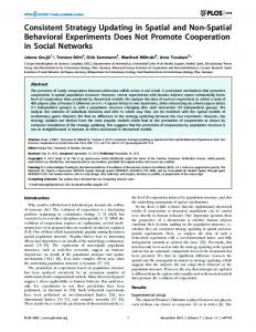
scopic models (i.e., those that study individual vehicle interactions) and macroscopic models (i.e., those that represent traffic as fluid and study only the behavior of some aggregated variables). We limit our attention to the latter models since those are the relevant ones for policy and economic analysis. A significant portion of the literature focuses on steady-state (or time invariant) representations of traffic. Stationary traffic conditions are represented by a fundamental diagram, which describes the possible states of a homogenous traffic stream in terms of three main parameters: density k (vehicles per unit length), speed v (distance per unit time) and flow q (vehicles per unit time). The fundamental diagram varies with the road characteristics, traffic composition and other environmental factors, but it has a basic shape represented in Figure 1.1a (see May [1990] for a literature review). As shown in the upper part of the figure, speed decreases monotonically with density (i.e., the number of vehicles in the road), with the decrease being steeper with larger densities when queues appear. This behavior is not surprising since commuters tend to keep smaller spacing between vehicles as speed decreases. Traffic flow is determined by speed and density through the identity q = kv; therefore, it first increases with density up to a maximum flow (called the capacity qmax ) and then decreases until the density reaches a maximum value (called the jam density kj ) when both flow and speed are zero; see the lower part of Figure 1.1a. The increasing branch of the q − k diagram is normally called the free-flow or uncongested regime, since the stationary states in this branch arise when no restrictions exist downstream of the road. The decreasing branch is called the congested or queued regime since its states describe the traffic stream inside queues caused by downstream restrictions. The decreasing branch is sometimes termed the hypercongestion regime in the economics literature and the term volume is also often used instead of flow.

6

1 Introduction For network design, planning and economic analysis, the usual goal is predicting

travel times. Many studies customarily use, instead of the fundamental diagram, some form of a link-based volume vs. trip time curve for that purpose. Volumetrip time curves give the average vehicle trip time as an increasing function of the volume/capacity ratio under stationary conditions; see Figure 1.1b. Mathematically, these functions can be derived from the uncongested branch of the fundamental diagram since the trip time for a link of length ` is `/v and the volume capacity ratio is q/qmax . These curves are often called link performance functions or volume-delay curves. Because of their convenience, link performance functions have become a standard tool of the network literature (see section 1.1.2), and many ad-hoc forms (not necessary consistent with the traffic fundamental diagram) have been proposed and tested empirically; see Branston [1976].2 There are, however, some important limitations that are not always clearly recognized in this representation of traffic. First, link performance functions represent steady-state behavior that cannot be assumed to hold during a full peak period. Hence, link performance functions estimated from time-dependent data may internalize not only the technological aspects of the road segments where they are estimated, but also features of its demand. Second, from a spatial point of view, these functions ignore spatial interactions between connected links (e.g., interactions at merges or diverges). Hence, their use on most network settings is unrealistic. Finally, volume-delays function can only represent adequately situations of mild congestion. When queues fill a link, experience and experiments show that longer travel times arise when flow declines, a result contrary to the link function prediction. Obviously, this limitation reduce the applicability of such functions since networks without spillovers are rare (i.e., the situations of interest are 2

By far the most widely used link performance functions are the BPR curves [Bureau of Public Roads, 1964].


7

normally those where large delays are experienced by commuters). To overcome these limitations, traffic models must explicitly consider the traffic dynamics. speed (v)

travel time (tt)

kj density (k)

v

flow (q )

qmax

qmax

(a) Fundamental Diagram

flow (q )

(b) Travel time-volume function

Figure 1.1. Steady-state traffic model.

Dynamic models allow for traffic conditions (e.g., flow, density and speed) to vary with location and time. The simplest and most widely accepted dynamic model is the kinematic wave (hereafter KW) model, first proposed by Lighthill and Whitman [1955] and Richards [1956]. This model assumes that traffic can be treated at the macroscopic level like a fluid and that the stationary fundamental flow-density diagram holds also under non-stationary conditions at every location and time. Transitions between different stationary states (e.g., between a free-flow and a queued situation) are represented by waves that propagate along the road segment. The KW theory – as originally presented by Lighthill and Whitman, and Richards – requires a burdensome mathematical apparatus to obtain solutions. This inconvenience has limited its use for practical applications, and several alternative approaches have been proposed. The most common simplification consists in assuming that the static volume-delay functions also apply to the dynamic case; i.e., that the travel time (or

8

1 Introduction

for that matter, the speed) of a vehicle entering a road is only a function of the road inflow at the time of entry. This is equivalent to assuming that congestion is a local phenomena and that no propagation of traffic conditions occurs on time or space (from now on, we call this the local congestion assumption). This simplification leads to clearly inconsistent behavior – for example, the classical Smeed’s paradox [Smeed, 1967] in which vehicles departing late in a low-flow cohort catch up a high-flow cohort that departed earlier, overtake them and arrive to the destination before them.3 To alleviate this problem, link performance functions have been amended to allow the travel time of an entering vehicle to depend on the link outflows and/or the occupancies (see Ran and Boyce [1996], chapter 12). However, Daganzo [1995c] shows the inconsistencies persist in any model where travel time depends in any way on the inflows or outflows. A model that explicitly accounts for flow propagation and avoids Smeed’s paradox is proposed in Mahmassani and Herman [1984]. In this model, density and speed change simultaneously and uniformly along the link with every change in the link inflow. Unfortunately, such assumption implies rather unrealistically that traffic conditions propagate in the forward direction instantly (i.e, that vehicle speed continues to be affected by following traffic) and this has undesirable effects too; see Newell [1988]. A more consistent treatment of traffic dynamics is obtained by representing each link as a bottleneck with a fixed capacity and a dimensionless (or point) queue forming upstream when link inflow exceeds capacity; see, for instance, Kuwahara and Newell [1987] and Kuwahara and Akamatsu [1997]. With this assumption, link travel time depends exclusively on link occupancy at the time of entry. Although these models do not suffer from Smeed’s paradox, they still yield wrong predictions when 3

Newell [1988] showed that the paradox never arises if the speed of vehicles is affected by congested conditions ahead of them, as in the KW model.


9

queues spillover across links; see Daganzo and Lin [1994]. Thus, even queuing models fail to represent adequately the macroscopic traffic behavior under heavily congested situations. Fortunately, Newell [1993] recently showed that the KW solution procedures can be simplified dramatically if (i) traffic is represented in terms of cumulative vehicle counts (instead of flows) and, (ii) a triangular fundamental q-k diagram is used. Under these assumptions, an alternative treatment based on standard queuing theory methods is possible, opening the door for the analytical treatment of some important problems. Daganzo [1994, 1995a] extend Newell’s ideas by including consistent models of merge and diverge interaction and an efficient approximation procedure for very large networks (the so-called cell transmission model ). Recent empirical evidence [Windover, 1998] has confirmed that the KW model captures the macroscopic behavior of queues quite realistically and provides estimates of overall vehicle delays in agreement with empirical observations. The KW model is known to have some limitations, but higher-order modifications to the KW model or alternative microscopic models based on car following theory do not necessarily present a better grounded representation of traffic [Daganzo, 1997] and have failed to provide better predictions of travel times [Brockfeld et al., 2003]. Newell KW procedure will be adopted throughout this dissertation. A detailed explanation of the theory is given in chapters 2 and 3.

1.1.2

Network models and equilibrium

Network models are used to simulate traffic behavior when different origins and destinations are linked through a series of routes. These models must recognize that vehicle flows on each route are not known a priori, since they are the result

10

1 Introduction

of commuters’ trip decisions. Commuters respond to congestion by choosing among different modes, routes and departure times. Since the focus of this thesis in on roadtraffic congestion, we shall restrict this review to models that incorporate route and departure time choice. The conceptual framework to analyze route choice under steady-state conditions was introduced by Wardrop [1952]. According to Wardrop first principle, users choose routes so as to minimize their individual trip cost. This behavior leads to an equilibrium situation in which the trip costs between each origin destination (OD) pair are equal in all used routes and larger on the routes not used; i.e., commuters do not have an incentive to change routes. The resulting pattern is normally called the user equilibrium. The user equilibrium differs from system optimum patterns where the minimum total travel time in the system is achieved as if an overseeing authority could direct all commuters. Wardrop’s principle is an oversimplification of reality because it assumes perfect information and utility-maximizing commuters that behave deterministically,4 but it is reasonable as a first approximation for rough planning analysis. Beckmann et al. [1956] proposed a mathematical optimization framework to solve Wardrop’s network equilibrium problem under static traffic conditions using link performance functions. Extensions of Wardrop’s principle to stochastic route choice have been provided in Daganzo and Sheffi [1977]. Extensions that consider multiple vehicle classes can be found in Dafermos [1980] and Daganzo [1983].5 Since the static models are not very satisfactory to represent situations of high congestion as mentioned in §1.1.1, dynamic traffic equilibrium has been an active area of research for the last two decades. Dynamic network equilibrium is both conceptually and computationally more difficult. A first conceptual complication stems from 4 5

Wardrop principle is a special case of Nash equilibrium. For a more through review of static network models see Patriksson [1994].


11

the fact that different definitions of equilibrium are possible under dynamic conditions, depending on the information available to the users. The natural generalization of Wardrop principle assumes that the routes chosen on each OD pair at each time of departure are those that minimize the experienced trip cost (which is now timedependent). This type of equilibrium, normally termed ideal or predictive dynamic user equilibrium (PDUE ), assumes that the dynamic evolution of traffic conditions is consistent day-after-day and therefore, that users can be aware (i.e., predict) of future traffic conditions at links visited downstream when selecting optimal routes at their origin. Smith [1993], Wie et al. [1995], Ran et al. [1996], Ran and Boyce [1996], Akamatsu and Kuwahara [1999], Tong and Wong [2000], Akamatsu [2001] and Huang and Lam [2002] provide different network models under this assumption. Since equilibrium route choice must be based on future traffic conditions this type of equilibrium problems are notoriously difficult to solve. Equilibrium is generally modelled through a set of discrete variational inequalities [Wie et al., 1995] or an equivalent non-linear optimization problem [Akamatsu, 2001; Ran et al., 1996]. In all cases, laborious numerical search procedures (e.g., Frank-Wolf -like decomposition) are required to solve the problem. Furthermore, route enumeration is normally unavoidable (when multiple destinations exist) since it is necessary to keep track of flow propagation along specific routes. Therefore, substantial computational effort is required even for medium size problems. Alternatively, simulation-based approaches can be used [Huang and Lam, 2002; Smith, 1993; Tong and Wong, 2000] but still some sort of heuristic is needed to update volumes in each path until equilibrium conditions are approximately met. An alternative representation of equilibrium, normally termed instantaneous or reactive dynamic user equilibrium (RDUE ), assumes that commuters choose routes

12

1 Introduction

at each time based on the current travel times prevailing on the network. Works in this class include Friesz et al. [1989] (extended in Wie et al. [1990]), Papageorgiou [1990], Janson [1991], Ran et al. [1993], Lam and Huang [1995] and Kuwahara and Akamatsu [1997]. This type of equilibrium is easier to solve since no prediction of future travel conditions is needed. For example, if one ignores the multi-commodity contraints, as done in Wie et al. [1990] or Papageorgiou [1990], the problem can then be formulated as a standard optimal control problem. A better approach solves a shortest path problem in each time interval [Kuwahara and Akamatsu, 1997]. Furthermore, route enumeration is not required. The assumption about instantaneous travel times, however, is not very realistic when commuters trip times are comparable in duration with the length of the rush. In a dynamic traffic setting, commuters also reschedule their departure times based on congestion levels. Anecdotal evidence suggests that this scheduling adaptation may have effects as important as route choice;6 notwithstanding, dynamic equilibrium models that explicitly consider commuter departure time choice have received less attention, perhaps because departure time equilibrium is more difficult to model. A framework to analyze departure-time choice was first proposed by Vickrey [1969]. Vickrey assumed that commuters have a preferred time of arrival to their destinations and schedule their departure (or arrival) times to avoid periods of high congestion at the expense of suffering a scheduled delay for arriving earlier or later than desired to their destination. Small [1982] provides empirical verification of this behavior. Vickrey analyzed equilibrium in a very simplified time-dependent scenario with a single bottleneck, a single destination and a fixed number of commuters (more details 6

The omission of timing changes can lead to incorrect predictions about the benefits of policy measures such as congestion pricing or capacity expansions. Small [1992] discusses the example of BART opening in San Francisco.


13

are given in chapter 2). Vickrey’s framework has been incorporated into network models with route choice in Kuwahara and Newell [1987], Bernstein et al. [1993], Wie et al. [1995], Ran et al. [1996] and Huang and Lam [2002]. These models inherit all the difficulties of route-choice PDUE models and need to be solved with heuristic and/or simulation-based techniques.7 A common limitation to all the equilibrium models above, however, is that they are based on traffic models that are not fully consistent. The models in Friesz et al. [1989]; Janson [1991]; Papageorgiou [1990]; Ran et al. [1993, 1996]; Tong and Wong [2000]; Wie et al. [1990] adopt some form of link performance function (link travel time is expressed as a function of link inflow rate, outflow rate and/or vehicle accumulation, depending on the model). Akamatsu [2001]; Bernstein et al. [1993]; Huang and Lam [2002]; Kuwahara and Akamatsu [1997]; Kuwahara and Newell [1987]; Smith [1993] adopt a network of point-queues bottlenecks. As mentioned in §1.1.1, none of these representations is a sound approximation for the spatial propagation of congestion. Unfortunately, no model of equilibrium has convincingly incorporated traffic behavior based on the KW model yet. Recent attempts can be found in Lo [1999], which proposes a formulation for the ideal route-choice user equilibrium based on Daganzo’s cell transmission model (no solution algorithm is proposed, though), and Kuwahara and Akamatsu [2001], which proposes an ad-hoc algorithm to solve the reactive equilibrium. However, no model yet combines commuter departure time choice with the KW model. 7

Note that departure time choice is only consistent with predictive equilibrium since it is based on the assumption that arrivals times at the destination can be predicted.

14

1 Introduction

1.1.3

Economic analysis: road pricing and investment

The ultimate objective of traffic prediction is controling the overall system so as to achieve an efficient use of the road infrastructure. This is specially important in the case of road networks since users tend to make decisions taking in account their individual trip costs, but disregarding the cost (i.e., delays) imposed onto other road users. This “selfish” behavior usually leads to more congestion than what would be optimal from a social point if everybody cooperated (what we called the system optimum). Pigou [1920] first brought up this mismatch and fathered the concept of a congestion toll as a way improve road usage. Since then, economists have long studied the possibilities of road pricing. Economic modelling, though, has been largely based on the steady-state representation of traffic, as typified by the early works of Walters [1961] and Mohring and Harwitz [1962]. The basic paradigm is schematized in Figure 1.2. It uses the link performance functions of Figure 1.1 reinterpreted as an average travel cost vs. traffic demand (or number of trips made during the rush hour) curve, AV C(q) in the figure. In agreement with the assumption of negative congestion externalities marginal cost is assumed to increase with demand as indicated by M C(q).8 At the same time, since traffic demand must logically depend on travel cost, a down-sloping demand curve D(q) can be defined reflecting both the individual average and marginal value of using the road. The equilibrium traffic volume, qU E is found at the crossing of the demand curve and the average cost curve. This equilibrium volume is higher than the social optimal usage, qSO , found at the intersection of the marginal cost curve and the demand curve. To reestablish the social 8

Cost are expressed as a function of traffic volume assuming an homogeneous monetary cost of time and considering vehicle operation costs independent of traffic level. As initially presented by Walters [1961], the cost curve also included a backward bending portion representing the congested branch of the fundamental diagram but, it is clear that for steady-state analysis this is not adequate.


15

optimum usage level, a toll equal to the difference in average and marginal cost at qSO can be imposed. The optimal investment can also be analyzed since the travel cost curve depends on the road capacity level and the cost of providing capacity (i.e., the construction cost) can be reasonably estimated; see Mohring and Harwitz [1962] and Keeler and Small [1977]. A basic result is that congestion tolls will cover construction and maintenance costs over the long run in the presence of constant returns in road construction and maintenance. This single road pricing/investment model has been further enriched by considering users with different values of times, possible indivisibleness on the provision of capacity, etc.; see Hau [1998] for a review. This basic static model can be also extended to network problems considering Wardrop’s user equilibrium and system optimum principles [Wardrop, 1952]. Under the assumption that congestion on each link is a function of its volume, the system optimum can be achieved by imposing on each link an optimal toll of the same form as in the single road case [Beckmann et al., 1956]. Network road pricing modelling has been further enriched in different ways. For instance, models have been proposed to include different types of users (i.e., trucks, cars), to analyze second-best situations where only a reduced set of roads is priced, and to analyze situations where other modes of transport are also available. Reviews of the state-of-the-art on network road pricing models can be found in Lindsey and Verhoef [2000] and Arnott [2001]. The reliance on the classical steady-state model, however, has tilted the economic analysis towards considering trip quantity as the only factor of analysis, focusing excessively on pricing as the only solution (Arnott [2001] offers a good critique). Dynamic settings have received less attention. The seminal work is Vickrey [1969] (already metioned above) where pricing and investment policies are evaluated under a time-varying congestion model represented by a single bottleneck queue. A

16

1 Introduction

Travel cost (tt)

MC(q)

D(q)

AVC(q)

toll

q

SO

qUE

flow (q)

Figure 1.2. Congestion pricing model. similar dynamic analysis is proposed in Henderson [1977] – later revisited and corrected in Chu [1992] – where a model of local congestion is used instead. Despite its highly idealized nature, Vickrey’s bottleneck model unveiled some interesting insights particular to the dynamic case. For instance, unlike in the static case where congestion tolls always penalize road users, a time-dependent toll payment can leave all the commuters as well-off as before while turning wasted time in the queue into toll revenue. Vickrey’s model has been extended to different scenarios (e.g., several parallel bottlenecks between a single OD pair, alternative modes), different demand assumptions (e.g., elastic mode-dependent demand, heterogeneous commuters) and different time-dependent toll policies (e.g., continuous toll, step toll); see Arnott et al. [1998] for a comprehensive review. More recent innovations include the analysis of mixed rationing/pricing schemes that prove to be Pareto improving for all road users [Daganzo and Garcia, 2000]. All these works are a substantial advance with respect to the traditional stationary analysis but their results are somehow limited because they do not explicitly consider spatial differences – congestion affects all commuters in a equal manner independently of their origins and destinations.


17

Kuwahara [1990] and Arnott et al. [1993a] extend Vickrey’s analysis to consider two separate origins and a single destination, but the predictions in these works are based on a traffic model with point queues, which still limits the validity of the results. Wie and Tobin [1998] present a network traffic equilibrium model with dynamic pricing on each link, but again their model of traffic behavior does not consider properly queue propagation. Work that combines dynamic pricing with traffic models that account properly for queue propagation in space and time appears not to be done.

1.1.4

Urban location theory

A further step on the study of congestion recognizes the intimate link between land-use patterns and traffic congestion. Residential location choices generate a need for mobility which produces congestion and congestion, in turn, affects residential locations. Because individual location decisions affect the cost of living at other locations through increased congestion, an inefficient equilibrium distribution of population (e.g., with excessive sprawl) may arise if the congestion externality is not properly internalized through adequate pricing or land-use regulations. The first models of urban location which explicitly incorporated congestion were proposed in Mills and de Ferranti [1971] and Solow [1973]. These work study the efficient provision of transportation infrastructure when congestion costs are properly internalized. The Mills/Solow framework abstracts from cumbersome network formulations and assumes a continuous mono-centric city where a distributed population travels to the CBD using a continuous network of radial roads. To represent traffic behavior, a model of local congestion is adopted where travel speed is only a function of the local traffic volume at each location (i.e., the number of vehicles crossing the

18

1 Introduction

location) and independent of the conditions at any other location. Analytical and simulation results show that excessive sprawl and excessive land devoted to transportation happen if congestion is not priced adequately. A variety of works extend the Mills/Solow analysis to include different economic aspects. For example, Oron et al. [1973], Henderson [1975] and Arnott and MacKinnon [1978] primarily focus on inefficiencies in land use for housing under different market structures; Sullivan [1983a,b] explicitly consider labor markets; Wheaton [1998] compares land regulation and congestion pricing; Akai et al. [1998] analyzes equilibrium when transportation in provided by a private agent. Invariably, all adopt the local congestion model of traffic. The results in all these works must be regarded with care for two main reasons, however. First, the local congestion model is highly unrealistic. As a result, the relationship between population sprawl and congestion are quite artificial. For example, it is easy to show that the level of congestion is dependent on the distance scale; i.e., if all the distances are doubled, the congestion cost are doubled. Therefore, results about optimal city size are irrelevant. Second, under the steady-state representation, the results are also clearly dependent on the order at which commuters are assumed to pass through each location, since this determines local traffic volumes and hence the congestion levels [Ross and Yinger, 2000]. For instance, the traditional Mills/Solow approach assumes that commuters join upstream users as they pass through their access location so that all commuters travel together and arrive to the common destination at the same time. On the other hand, Yinger [1993] assumes that commuters depart at the same time so that people at different location travel in different groups, or cohorts, and arrive at the destination ordered by distance to the destination, leading to an equilibrium location pattern different from those of Mills and Solow. To

1.2 Dissertation overview

19

make timing decisions endogenous, Ross and Yinger [2000] incorporates Henderson’s model of dynamic equilibrium into the urban location problem, but it is concluded that no reasonable timing equilibrium can arise. This is yet another indication that local congestion is inadequate for the analysis. In summary, finding an adequate way of incorporating a sensible model of flow propagation and commuter trip timing into the equilibrium model of urban location continues to be a challenge.

1.2

Dissertation overview

1.2.1

Scope

The literature review in the previous section shows that substantial effort has been devoted to the study of congestion in various fields. Although progress has been made in many areas - specially in the modelling of traffic dynamics - there are still substantial needs for improvement. The following four needs will be addressed in this thesis: • Models of morning commute need to better incorporate congestion propagation. The available models of traffic equilibrium adopt unrealistic assumptions about traffic behavior. Either they ignore the spatial effect of queues or they assume that commuters are not spatially differentiated. Incorporating a realistic model into the network equilibrium analysis that can capture adequately the effect of physical queues will help addressing the aforementioned limitations. • Models of morning commute need to incorporate commuters trip tim-

20

1 Introduction ing decisions. Insights on the effects of departure time choice on traffic equilibrium patterns are very limited. This is unfortunate since trip rescheduling is a likely commuter reaction to many policy measures. Since departure time decisions differ by location, it is necessary to extend the analysis of network problems to include departure time choice. • Models of morning commute need to focus on stylized scenarios. Dynamic network equilibrium modelling has focused excessively on the development of algorithms rather than on the study of solutions; i.e., in the qualitative behavior of congested systems as a whole. The ‘algorithmic’ approach turns out to be rather inadequate to guide policy. Solutions can only be obtained through cumbersome computer-based simulation due to the complexity (and details) of network problems. From these solutions which are only particular to the scenario simulated, it is very difficult (if not impossible) to draw general qualitative insights about the behavior of congestion, which would be necessary to guide taxation and policy. Simplified scenarios that allow for the expression of the system behavior as a function of a few significant parameters and lead to analytical solutions may shed more light about the fundamental behavior of congestion. • Economic theory of urban location needs to revisited. As shown in §1.1.3 and §1.1.4, the economic models of congestion have been largely based on steady-state and local-congestion assumptions. As a result, these models fail to adequately represent the true spatial behavior of congestion. Consistent relationships between the cost of congestion and the distribution of population need to be developed from realistic traffic models, such as the KW model, so that they can be further used for economic analysis.


21

The objective of our research is to relax as much as possible these four limitations. We develop a general model of the morning commute, which explicitly considers both realistic traffic behavior and commuters’ departure time decisions in response to congestion. In addition, the dependence of departure time decisions and the distribution of population is explored. We seek to use the model to derive qualitative insights about the behavior of traffic in urban areas that will be valid in general. Therefore, the analysis will focus on selected geometries which include symmetries that allow for analytical solutions. Mono-centric cities, where commute is bound exclusively to a central business district (CBD) will be the main focus.

1.2.2

Main contributions

The main contributions of this research include: • The development of the first model of traffic equilibrium which combines departure time choice and a realistic model of traffic flow. This model combines Vickrey’s model of departure time choice with Newell’s model of the KW theory. • The development of an analytical procedure to solve the departure-time equilibrium for: (a) simple network with two-origins, (b) many-to-one tree networks. • The theoretical analysis of the effects of ramp metering and capacity expansion when departure time is an issue. This analysis reveals unexpected situations where ramp-metering can be beneficial, and others where the provision of more freeway capacity or storage can be counterproductive. • The study of the relationship between congestion cost and population distribution for mono-centric cities. This study is based in both discrete (networkbased) and continuous models.

22

1 Introduction • The development of closed-form expressions that link congestion costs to location and spatial population distribution. These formulae are structural relationships since they make endogenous commuters timing decisions and traffic dynamics; hence, they can be generally applied to study other more general urban problems.

1.2.3

Organization

The thesis is organized in a series of self-contained chapters. Chapter 2 presents a first model that explicitly considers the most important determinants of congestion behavior during the morning commute: different commuter origins, merge interactions and queue spillovers. We examine the simplest possible network (2 origins and one destination) exhibiting the three important features. This model can be used as a building block for the analysis of more complex, single-destination networks with departure-time choice. Chapter 3 extends the analysis to the case of a long homogeneous freeway. This model is relevant since a long homogeneous freeway is the logical unit of analysis for mono-centric cities with ring-radial street networks. We develop an exact analytical procedure that can be used to model morning commute traffic evolution in long corridors. The analysis of congestion in monocentric cities is presented in chapter 4. Both a discrete and continuous formulation are investigated. General closed-form solutions are proposed that allow the quantification of commuting costs as a function of location and population distribution. The focus of chapters 2, 3 and 4 is on concepts, qualitative insights and policy analysis, rather than in methodologies. For that purpose, we adopt some simplifying assumptions that allow direct analytical treatment; e.g., that the networks are homogenous and commuters have the same desired arrival time to the destination. Chapter 5 - which can be


23

considered a technical addendum to the previous chapters - extends the analysis to more general instances where the network is nonhomogeneous and commuters have different desired arrival times. This chapter provides additional insight and discusses the difficulties one encounters in the design of solution algorithms for the morning commute problem over general networks. Finally, chapter 6 presents some conclusions and discusses possible extensions of the work in this thesis.

25

Chapter 2 A Simple Network Model Vickrey [1969] describes the first traffic model where commuters can adapt their departure time to avoid periods of high congestion. The model is very simple – a single bottleneck with a fixed number of commuters – but also very revealing of possible policy actions for congestion reduction. Because of its appeal and simplicity, Vickrey’s model has been extensively analyzed under different demand assumptions [Arnott et al., 1993b; Daganzo, 1985; Hendrickson and Kocur, 1981; Newell, 1987; Smith, 1984] and has also been adopted to analyze various toll policies [Arnott et al., 1990; Daganzo and Garcia, 2000; Laih, 1994]. The model, however, only applies to cases where congestion is concentrated at a single location, affecting all commuters equally. These conditions are violated when the access network is itself congested. For example, freeway queues caused by bottlenecks often spill over long distances imposing different penalties on its access points. Obviously, network effects should be investigated. This chapter introduces a network model that integrates Vickrey’s theory with a realistic traffic flow model [Newell, 1993] and a reasonable merging mechanism [Daganzo, 1995a]. Our ultimate goal is the qualitative understanding of the relationship

26

2 A Simple Network Model

A (N(A))

qmax

B (N(B))

qmax

M

(qmax,kj) qD(t) D

l

Figure 2.1. Homogeneous 2-origin network. among congestion, departure time choice and the spatial distribution of population for the morning commute, recognizing the networks are congested and have different origins. We consider the simplest network with all these relevant characteristics. It consists of two origins, one destination and two links merging into a third, as shown in Figure 2.1. The chapter is structured as follows. Section 2.1 introduces relevant background and discusses the single bottleneck (Vickrey) model. Section 2.2 presents the equilibrium and the traffic model for the two origin network. Section 2.3 presents the results. Section 2.4 compares the solutions with those obtained under point-queue assumptions. Finally, section 2.5 discusses policy implications and relates them to earlier work.

2.1

The single bottleneck model

It is commonly assumed that traffic conditions during the morning commute are similar day-after-day. Commuters, aware of these, choose their departure time to minimize their individual trip cost, which consist of a trip-time component and a

2.1 The single bottleneck model

27

schedule penalty. The latter is associated with the actual arrival time at the destination relative to a preferred arrival time. In the case where the only traffic restriction is a single bottleneck of capacity qD with no delay elsewhere, it is customary to express commuter decisions as a function of the preferred passage time through the bottleneck or deadline. If wt is the deadline for the commuter that passes the bottleneck at time t and we express costs in units of trip time, then the trip cost for that commuter is

c = τ + p(t − wt ),

(2.1)

where τ is the trip time and p(·) is a schedule penalty function such that p(·) ≥ 0 and p(0) = 0. It will be assumed here that p(·) is piecewise linear and V-shaped, where e and L are the positive conversion rates for earliness and lateness into trip time; i.e.,

p(s) =

   −es if s < 0   Ls

(2.2)

if s ≥ 0.

Normally, earliness is preferable to both queuing and lateness, i.e., e < L, e < 1 [Small, 1982]. The objective is then determining an equilibrium schedule of departures from a single origin such that no commuter/vehicle would have an incentive to change its departure time given the queues that resulted from the equilibrium. The model also applies to multiple origins if all access routes to the bottleneck are uncongested and pass through a common point, O; i.e., point O can be modelled as the single origin. The solution can be represented by means of continuous cumulative plots, assuming that the number of commuters is so large that vehicles can be treated as a continuous variable; see Figure 2.2. W (t) expresses the cumulative number of commuters wishing to pass the bottleneck by time t, and it will be called the deadline

28


curve. It will be assumed that W (t) is S-shaped, with slope greater than the capacity qD during some interval so that a queue must necessarily develop. W (t) is a step function if all the commuters have the same deadline, as shown in Figure 2.2a. Then, the objective is finding an equilibrium curve of cumulative arrivals at the common point O, AO (t) – or equivalently the curve of cumulative virtual arrivals at the bottleneck, A(t) = AO (t − tOD ) where tOD is the fixed uncongested trip time from O to the bottleneck location, D.1 According to standard queuing analysis, the curve of cumulative departures from the bottleneck, D(t), is the highest curve with slope less than or equal to qD such that D(t) ≤ A(t).2 Under a FIFO (first-in-first-out) queue, the delay τ for any given vehicle number is the horizontal distance between curves A and D. Likewise, the scheduled delay s is given by the horizontal distance between D and W if vehicles depart from the bottleneck in the order of their deadlines. It is known that if the penalty function p(·) is convex and common to all commuters, the solution exists [Smith, 1984] and is unique [Daganzo, 1985]. Furthermore, in the equilibrium solution, vehicles depart from the bottleneck in the order of their deadlines. An example of such equilibrium is represented in Figure 2.2 both for the case when commuters have a common deadline (Figure 2.2a) and when they do not (Figure 2.2b). Both solutions exhibit a unique queuing episode with two clearly differentiated phases. In the first phase, commuters depart from the bottleneck earlier than desired and queuing delay increases with vehicle number at a rate that precisely compensates for the reduction in earliness. Therefore, the slope of A(t) is given by qD /(1 − e). In the second phase, commuters depart from the bottleneck later than 1

A vehicle virtual arrival time to D is the time at which the vehicle would have passed D if it had travel unhindered from O to D. 2 In queuing lingo, the terms arrivals and departures refer to the bottleneck. Therefore, they have the reverse meaning assigned to them in the economics literature where arrivals to the bottleneck correspond to the departures from the origin and vice-versa.

2.1 The single bottleneck model

29

desired and queuing time declines with vehicle number to compensate for increasing lateness penalties. As a result, the slope of A(t) is also given and equal to qD /(1 + L). Note that the vehicle arriving on time experiences the highest delay as given by the length of segment AO, |AO|, in Figure 2.2. In the single deadline case of Figure 2.2a, |AO| is the common cost suffered by all commuters. If ts and tf are the times when the queue starts and vanishes, equilibrium requires |AO| = Ltf = −ets . Furthermore, if we use N to denote the number of commuters who queue, then N = qD (tf −ts ) since all these commuters depart when the bottleneck is at capacity. In the single deadline case, N is known (i.e., all the commuters suffer delay), therefore these three equations define the three remaining unknowns: |AO|, ts and tf . Since the slopes of A(t) above and below AO are given, it follows that there is only one possible geometry for the equilibrium curves. Figure 2.2a shows that the number of commuters departing early at equilibrium is N L/(e + L) and the number departing late is N e/(e + L). One can also see that the common cost is |AO| = N eL/(e + L). Finally note that the equilibrium delay for a commuter departing at time t, τ (t), is

τ (t) =

   |AO| + et = e(t − ts )

if t < 0

,

(2.3)

  |AO| − Lt = e(tf − t) if t ≥ 0

which precisely balances the schedule penalty as required.

Consideration shows that a similar geometric pattern is an equilibrium for any S-shaped deadline curve; see Figure 2.2b. The main difference is that in this case not all the commuters queue; therefore, one also needs to find N . Most of the existing literature deals with fixed-capacity bottlenecks, but the analysis can be extended to variable capacities, qD (t). Then, ts , tf and A(t) can be

30


# A(t)

N [e/(e+L)] O

t

D(t)

A

t

s

N [e/(e+L)]

qD/(1+L)

D(t)

A

tf

A(t)

.

qD/(1+L)

qD/(1-e)

#

tf

O

t

qD/(1-e) N [L/(e+L)]

qD

N [L/(e+L)]

qD W(t)

W(t) ts

ts (a) Common deadline

(b) Different deadlines

Figure 2.2. Single bottleneck equilibrium solution (fixed capacity). determined as before since (2.3) continues to hold. This means that in any equilibrium, such as that shown in Figure 2.3a, the horizontal separation between A and D at # = D(t) continues to be given by (2.3). Therefore, if the equilibrium diagram is rescaled vertically by means of the transformation # = D−1 (t) which makes the departure rate equal to 1 at all times, i.e., D−1 (D(t)) = t , then we recover Figure 2.2a. This is shown in Figure 2.3b. The re-scaled arrival curve, T (t) = D−1 (A(t)), now returns the departure time td (on the vertical axis) as a function of the arrival time ta (on the horizontal axis). We shall refer to T (t) as the arrival-departure schedule curve (or A/D curve) to differentiate it from the actual equilibrium arrival curve, A(t). The invariance of the rescaled diagram with respect to qD (t) will become useful later. It should be remembered that the single bottleneck model does not apply if delays experienced by vehicles entering the network at different locations are different, as is normally the case for freeway networks. Unfortunately, no existing model addresses

2.2 Two-origin departure-time equilibrium and realistic traffic behavior

# (or t)

#

W(t) tf

A(t)

T(t)

O

N

t

qD(t)

t

td

.

A

O

t(td)

td(ta) .

D(t)

ts

tf

qD=1

ta

A

W(t)

31

ta,td

D(t) ts (a) Equilibrium solution (Time-dependent capacity)

(b) Re-scaled Solution

Figure 2.3. Single bottleneck equilibrium solution (time-dependent capacity). the three key effects required to model a simple freeway: multiple origins, merging interactions and queue spillovers. The next section describes a first step in this direction.

2.2

Two-origin departure-time equilibrium and realistic traffic behavior

2.2.1

Problem formulation

We shall consider here the simplest network exhibiting all three effects; see Figure 2.1. On this network, N (A) and N (B) commuters travel everyday from origins A and B to a common destination D. The routes from these origins merge at an intermediate location, M , and share a final link M D of length `. A bottleneck of (possibly

32


time-dependent) capacity qD (t) may exist just upstream of D and queues may form on the common link and spill over the merge.3 For simplicity, we assume that: (1) the network is homogeneous (i.e. its three links have the same characteristics), (2) all commuters have the same deadline and penalty function (i.e., commuters are only distinguishable by their origin). Generalizations for networks with non-homogeneous links and different deadlines are discussed in chapter 5.4 We express our solution in terms of origin-specific cumulative inflows (or cumulative departures from each origin) and cumulative outflows from point D (or arrivals to the destination). We can ignore free-flow trip times in our analysis, since those are fixed for each origin and independent of the time of arrival. In this case, the solution is defined by the curves {A(r) (t), r = A, B}, which represent the virtual cumulative arrivals at point D for each origin – instead of the actual cumulative departure curves (r)

from origins A and B – and {DD (t), r = A, B}, the cumulative departures from D. (From now on, superscripts identify the origin to which the variable or function refers, while subscripts refer to the physical location over which the variable or function is (r)

defined. Furthermore, a(r) and dD represent the time-derivatives or flows respec(r)

tively; e.g, dD (t) is the flow at D of commuters from origin r.) Delays – instead of (r)

actual travel times - are given by the horizontal separation between A(r) and DD ; −1

(r)

i.e., τ (r) = t − A(r) (DD (t)). The actual departure curves from the origins can be obtained by shifting the virtual curves back in time by the origin-specific free-flow trip (r)

times; i.e., Ar (t) = A(r) (t + `rD /vf ) where `rD is the total distance from origin r to (r)

point D and vf the free-flow speed. Actual trip times are given by τrD = τ (r) +`rD /vf . A possible assignment pattern (not necessarily in equilibrium) is presented in 3

The flow restriction could be due to a variable inflow from another ramp (not depicted in Figure 2.1) very close to D. 4 A summary of the notation used in this chapter and throughout the dissertation can be found in appendix B.


33

Figure 2.4. The two origin-specific diagrams of Figure 2.4a can be conveniently superimposed, by adding vehicle numbers, to analyze the traffic behavior on link M D as shown in Figure 2.4b. The curves DM and DD represent the actual departure curves from M and D, respectively. The proportion of departures by origin at time (r)

(r)

(r)

t is defined as αD (i.e., dD (t) = αD (t)dD (t)). Under FIFO conditions, the delays experienced in link M D, τM D – given by the horizontal distance between DM and DD – must be equal for both origins. Furthermore, the proportion of vehicles departing (r)

(r)

from D must be the same when the vehicles passed M , i.e., αM (t − τM D (t)) = αD (t). Finally, it is convenient to consider the re-scaled origin-specific A/D curves T (A) and T (B) constructed as explained in §2.1 since these curves allow recovering the actual experienced delays. Total delays are given by the horizontal distance between T (r) and DD ; delays in each approach upstream of the merge by the horizontal distance between T (r) and DM . We will make extensive use of this construction when analyzing the solutions.

2.2.2

Traffic dynamics

The equilibrium solutions must then be consistent with both link and node dynamics. Basically, the two phenomena that affect the traffic solution are the queuing behavior on link M D and the merge interactions. Traffic in link M D is modelled as in the simplified kinematic wave (KW) theory proposed in Newell [1993]. According to the theory, traffic obeys a triangular fundamental relationship linking flow q with density k defined by three parameters: a fixed free-flow speed (vf ), a maximum flow or capacity (qmax ) and a jam density (kj );5 see Figure 2.5a. Newell shows that the delay-based traffic problem can be solved as a standard problem with the modified 5

Jointly they define a wave speed w which represents the unique speed at which flow disturbances propagate upstream within a moving queue.

34


#

DD(A)

(A)

A(A)

DM

DD(t)

DM(t) T(B)(t)

DD(B) DM(B) A

T(A)(t)

(B)

tMD

tMD t t

t

(B)

(A)

t

(B)

(A)

t

(a) Origin-specific assignment

(b) Aggregated re-scaled assignment

Figure 2.4. Traffic assignment with 2 origins. Cumulative plot representation. fundamental diagram of Figure 2.5b, which has the same qmax and kj but vf = ∞. The traffic model is completed by defining how vehicles interact at the merge. We will use the rules in Daganzo [1995a]. These are depicted in Figure 2.5c and explained later. Physical queues dynamics: The delays in link M D must be predicted since we must guarantee that commuters from different origins passing M at the same time incur the same delay on link M D (i.e., queues are FIFO). Physical queue are relevant in link M D since the common delays on the link depend on the queue spilling over the merge section or not. For links AM and BM , physical queues are not an issue because the delays suffered in these links are always common to all the commuters from the same origin. D According to Newell, a capacity curve at M , DM , is defined from the departure

curve at D, DD , by the shift,


35

(a) Original q-k diagram (c) Merge q-k model

q

qmax d M( A)

vf

-w

queues at A (A)

kj (b) Transformed q-k diagram

q’

queues at B

1

vf = ¥

qmax -w’=-qmax/kj

(B)

a /a

k

no queues

qM

d M( B )

k’ kj

Figure 2.5. Traffic flow model and merge model [Newell, 1993].

D DM (t) = DD (t −

kj qmax

`) + kj `

(2.4)

This capacity curve tracks the effects of the backward moving queue on the entrance of link M D and sets an upper bound to the cumulative number of commuters that can pass M by time t; see Figure 2.6. The actual cumulative curve of vehicles passD ing through M , DM (t), is the lower envelope of DM and the cumulative number of

commuters who would have passed M in the absence of a queue, which is determined by upstream demand. In our case, the upstream behavior depends on the merge behavior. Merge interactions: The flows from the two approaches must share the downstream capacity according to some pre-specified merging rules. Daganzo [1995a, 1996] pro(A)

(B)

poses that the upstream flows from each merging approach – dM , dM – must be a

36


function of the capacity of the upstream approaches (i.e., qmax ), the available capacity downstream (qM ) and some approach-specific priority ratio – α ˜ (A) , α ˜ (B) – where α ˜ (A) + α ˜ (B) = 1. For the case of interest here where the (time-dependent) downstream capacity is given by qM (t) = dD M (t) < qmax , the upstream approach capacities do not play a role and the rules reduce to the following two: (1) during periods when there are no queues upstream of M , arrival flows equal (A)

(B)

discharge flows and dM = dM + dM ≤ qM (t); (2) when there is a queue on approach r, then dM = qM (t) and the departure ratio (r)

(r)

˜ (r) . αM ≡ dM /dM ≥ α (A)

(B)

It follows from (2) that when there is a queue in both approaches, then dM /dM = α ˜ (A) /˜ α(B) . These rules are illustrated in Figure 2.5c. A more detailed description of the dynamics of the merge section for more general cases can be found in Daganzo [1995a, 1996] and in chapter 3, §3.2. Delay-based representation: In our case, it is convenient to express all the traffic feasibility conditions in terms of the some candidate equilibrium departure curves (A)

(B)

from D – DD and DD – and the origin-specific equilibrium delays – τ (A) and τ (B) – indexed by time of departure. As we shall show later in §2.2.3, equilibrium conditions are easily expressed as a function of these functions. To express behavior in link M D as a function of delays, first note that DD will be such that dD (t) = qD (t) if max{τ (A) (t), τ (B) (t)} > 0

(2.5)

D Furthermore, note that DM (t) − DD (t) is an upper bound for the length of the queue D at M D at time t. Hence, the horizontal separation between DM and DD , νM D (t),


(a) Newell Shift

37

(b) Delay-based procedure

#

#

D

D

DM (t)

DM (t) .

nMD(t)

.

max

T (t) DD(t)

nMD(t) o

o

(A)

(B)

max{t ,t }

t

t

(kj)l (kj/qmax)l .

DD(t)

.

Figure 2.6. Newell’s KW procedure. is also an upper bound for the delay on link M D for any given departure time (we call νM D (t) the maximum delays or M-delays). We can compare the delays τ (A) and τ (B) with νM D in an attempt to infer the actual delays τM D and hence, the actual departure curve from M , DM . Since 0 ≤ τM D ≤ νM D and 0 ≤ τM D ≤ max{τ (A) , τ (B) } (because of the FIFO discipline), then three main situations cases can arise, as given by

dM (tM ) =

    dD  M   

if νM D = τM D ≤ max{τ (A) , τ (B) }

qmax if τM D < max{τ (A) , τ (B) } < νM D       min{a(A) + a(B) , qmax } if τM D = max{τ (A) , τ (B) } < νM D

(2.6)

The first equality corresponds to the case with queues spillovers at M ; the second, to the case with no queue spillover at M but queues at the upstream approaches; the

38


third, to the case with queues only downstream of M . Based on (2.6), the actual curve DM and the delays τM D can be defined as function of max{τ (A) , τ (B) } in the following graphical manner (see Figure 2.6): draw the curve T max such that the horizontal distance between T max and DD for each t corresponds to max{τ (A) (t), τ (B) (t)} (i.e., T max is the A/D curve for the maximum delays); then, obtain DM as the lower D envelope of DM and the higher curve underneath T max with slope ≤ qmax . The delays

τM D are given by the horizontal distance between DD and DM for each departure −1 time t, i.e., τM D (t) = t − DM (DD (t)).

The merging rules must also be expressed in terms of our candidate departure and delay curves. When τ (r) (t) > τM D (t), vehicles from approach r departing from D at t experience delay upstream of the merge. Hence, in view of merge condition 2, (r)

they must enter the merge in a proportion αM ≥ α ˜ (r) . Since this proportion must be preserved at D, we can write:

(r)

τ (r) (t) > τM D (t) ⇒ αD ≥ α ˜ (r)

(A)

(2.7)

(B)

α(A) , α ˜ (B) ). τ (A) (t) > τM D (t), τ (B) (t) > τM D (t) ⇒ (αD , αD ) = (˜

(2.8)

Condition (2.7) applies when the merge is at capacity with one congested approach and (2.8) with two. When the merge is non-congested, any proportion of flows is (r)

allowed. Finally, if τ (r) (t) < τM D (t) the solution is only feasible if dD (t) = 0.

2.2.3

Equilibrium conditions

Departure time-equilibrium requires that the trip cost for commuters in the same origin r must be equal for any chosen arrival time and equal or larger for any other non-chosen times. The traffic-equilibrium problem could be solved by considering the


39

arrival curves {A(r) , r = A, B} as the unknowns since these define through the traffic (r)

model unique {DD , r = A, B} and {τ (r) , r = A, B}. One would need to iterate on the A(r) ’s until finding costs that satisfy the equilibrium criterion. The equilibrium solution, however, can be more easily obtained in one takes in account some properties of the solution. Property UE(1) (or Parametric representation of equilibrium). The equilibrium delays (or trip times) for each origin, τ (r) , are uniquely determined by the time of (r)

arrival of the first commuter from the origin suffering any delay, ts , and so is the equilibrium cost, C˜ (r) . Proof. Recall that in the single origin the equilibrium delay τ (t) was affected by D(t) through ts and tf . Obviously, the same simple principle applies now but with origin(r)

specific ts

(r)

and tf . From equation (2.1), the equilibrium cost for the commuter

(r) (r) arriving at ts is given by C˜ (r) = p(ts ) and thus,

τ (r) (t|ts(r) ) = C˜ (r) − p(t) = p(ts(r) ) − p(t).

(2.9)

Property UE(1) suggests the following solution approach. Choose initially a set (r)

{ts , r = A, B}, which defines unique origin-specific equilibrium delays (or travel times), {τ (r) ,r=A,B}. Then, find the traffic-feasible arrival and departure processes (r)

(r)

{A(r) , DD , r = A, B} which are consistent with the {ts , r = A, B} and {τ (r) ,r=A,B}. We can use the delay-based traffic formulation in §2.2.2 to do this. This traffic assign(r)

(r)

(r)

ment {A(r) , DD , τ (r) } will be an equilibrium but the total outflows {DD (tf ), r = A, B} may not match the populations N (r) , r = A, B. Hence, we would have to (r)

(r)

(r)

change the ts ’s until {DD (tf ), r = A, B} are equal to {N (r) , r = A, B}. An immediate corollary of property UE(1) is

40


Property UE(2) (or sequential ordering of delays). Given an ordering by origin (r) of initial times ts (or equivalently, of costs C˜ (r) ), the equilibrium trip times for any

other departure time follow this same order, i.e., ∀r, s C˜ (r) > C˜ (s) ⇐⇒ τ (r) (t) > τ (s) . Property UE(2) states that the maximum delays experienced by any commuter for a given departure time, max{τ (A) , τ (B) }, necessarily coincide with the equilibrium delays for one of the origins. This suggests that the solution procedure can be streamlined even more by considering only equilibrium solutions where the full capacity available at D is utilized during the interval Π = [ts , tf ] given by the single origin bottleneck solution with total population N (A) + N (B) , i.e., the combined departure curve at D, DD , coincides with that of a single origin problem. This is intuitive since our network model allows un-delayed travel from both origins when section D is under capacity (therefore, commuters independently of the origin they come from would have an incentive to use the full capacity at the preferred times).

2.3

Equilibrium analysis

We consider the single deadline problem and analyze it in two phases: (i) cases with no bottleneck restriction at D (qD (t) ≡ qD = qmax ) where queues cannot form on link M D and merging effects dominate, and (ii) cases with time-dependent flow restrictions at D (qD (t) ≤ qmax ) where queue spillovers can affect performance.

2.3.1

No downstream restrictions (Merging effect)

When no restrictions exist downstream of merge M , no delays can arise beyond it. Therefore, we can ignore link M D and treat M as if it was the destination us(r)

(r)

ing DM (t) ≡ DD (t), αM (t) ≡ αD (t). In essence, the system is modelled as a pair

2.3 Equilibrium analysis

41

of single-origin bottlenecks with departure rates coupled by the merging rule. As mentioned in §2.2.3, it is logical to consider equilibrium solutions in which the aggregated departure curve DM is given by the single bottleneck solution with capacity qD and total population N (A) + N (B) , i.e., where the merge is saturated only during the preferred interval Π = [ts , tf ] of Figure 2.2a. (A)

(B)

Since DM is given, the capacity shares {αM (t), αM (t)} need to be found. If we further consider that only one queuing episode can occur on each approach, the solution is as shown in Figure 2.7a. The figure displays the arrival and departure pattern on the two approaches separately. Commuters from one origin (B in the figure) flow through the bottleneck during an interval when the other approach is (B)

˜ (B) . queued. Therefore, from (2.8), they use a fixed share of the capacity αM (t) = α The solution for B -users is a single bottleneck equilibrium with population N (B) (B)

and capacity α ˜ (B) qD ; see the bottom part of Figure 2.7a, curves DM and A(B) . Commuters from A flow at full capacity qD when the approach B is not active and at a reduced capacity α ˜ (A) qD otherwise. The solution for A-users is also a single bottleneck equilibrium, albeit with time-dependent capacity; see the top part of Figure 2.7a, (A)

curves DM and A(A) . The two diagrams of Figure 2.7a can be re-scaled and superimposed following the procedure explained in §2.2.2 to show the A/D curves for both origins and the common departure curves on a single diagram, see Figure 2.7b. The quantities in (A)

(B)

parenthesis following each colon are {αM (t), αM (t)}. The curves on the figure must be similar, as shown, since commuters share a common deadline and penalty function. Commuters from A experience the same commuting cost as if everybody had the same origin, since AO is equal in length to the corresponding segment of a single bottleneck solution with population N (A) + N (B) . Commuters from B, however, experience a

42


#

W(t)

(A)

A (t)

(A)

qD

A N

o

O

(A)

a(A)qD

DM

B O

A (t) a(B)qD

t (t)

. (A)

N +N A

B t(B) t

N

W(t)

(A)

qD (B)

#

T (t) (B) T (t)

(B)

(B)

DM (t)

(a) Origin-specific solution

O (B)

qD:(a(A),a(B)) N /a

(A)

(B)

t

. qD:(1,0)

DM(t)=DD(t)

(b) Aggregated re-scaled solution

Figure 2.7. Equilibrium solution, no queues in link M D. reduced cost, |BO|. From the figure, it is clear that B-commuters experience less cost if N (B) /˜ α(B) < N (A) /˜ α(A) . The reverse is true if N (B) /˜ α(B) > N (A) /˜ α(A) . The worst case arises if N (B) /˜ α(B) = N (A) /˜ α(A) when all commuters experience the highest cost. The best case arises if α ˜ (A) = 0 or 1 (complete priority) since one of the origins experiences the least possible cost. These results have an economic interpretation. Since the capacity of M is a scarce resource, commuters impose onto each other an external cost (delay) as they jockey for their preferred departure times. In the single bottleneck scenario, everybody is affected equally by the actions of the others and the result of this game is a symmetric equilibrium. A saturated merge, however, allocates its capacity in fixed shares – α ˜ (A) and α ˜ (B) – to the two approaches, which insulates B-drivers from actions of A-drivers and vice-versa. This allows one part of the population to reduce its cost by traveling at the most desired times. The effect can be exploited by manipulating (˜ α(A) , α ˜ (B) ),


43

proving that Pareto-improving ramp metering schemes exist for single-destination freeways with time-elastic demand. These is further discussed in the final section.

2.3.2

Downstream restrictions (Spillover effect)

Let us now assume that qD (t) ≤ qmax , with the possibility of spillovers from link M D. A feasible equilibrium can be found in a sequential manner. Figure 2.8 illustrates the steps for the case of a permanent restriction, qD < qmax , but the solution is general for any time-dependent qD (t). Step 1 : Aggregate departure curve and maximum delay. As before, we look for solutions in which the aggregate departure curve DD is given by the single bottleneck solution with capacity qD (t) and total population N (A) + N (B) ; see Figure 2.8a. This defines the duration of the queuing episode, Π = [ts , tf ]. By virtue of Property UE(2), necessarily one of the origins flows at both ts and tf . We shall assume that A-vehicles (A)

discharge uninterruptedly in the interval Π(A) ≡ Π (i.e., ts (B)

that B-vehicles discharge in an interval Π(B) ⊆ Π (i.e., ts

(A)

= ts ,tf

= tf ) and

(B)

≤ tf ) possi-

≥ ts , tf

bly with interruptions. Of course, The roles of the origins can be reversed and we show below that this depends on the population-to-priority ratio. The equilibrium (A)

delay function for origin A, τ (A) (t) = max{τ (A) (t), τ (B) (t)} , is obtained from ts

and

(A)

tf ; i.e., τ (A) coincides with the single origin delays. This can be expressed graphically in conjunction with curve DD by means of an A/D curve T (A) such that the horizontal difference between T (A) and DD for any departure time t is the A-delay: −1

τ (A) (t) = t − T (A) (DD (t)); see Figure 2.8a. Neither DD nor T (A) are cumulative counts for A-vehicles since DD gives the cumulative count for A and B -vehicles together.

44


Step 2 : Delays on the common link. Since the aggregate departure curve DD and the maximum delays, τ (A) , are given, we can use the procedure explained in §2.2.2 to obtain the actual delays on link M D, τM D : first, shift DD according to (2.4) to D obtain the capacity curve at M , DM , and the M-delays, νM D (t) (see Figure 2.8b);

then, obtain the curve of cumulative flows through M , DM , as the lower envelope D of DM and the higher curve underneath T (A) with slope ≤ qmax . The horizontal

difference between DM and DD is the actual delay τM D (see Figure 2.8c). These delays are highlighted by the shaded area of the figure. (B)

Step 3 : Solution for secondary origin (B). We first look for a starting time ts (A)

>

(B)

ts = ts . For each candidate ts , the equilibrium delays τ (B) are given. Thus, we can again define a curve T (B) such that the horizontal difference between T (B) and DD gives directly the equilibrium delay for origin B (see Figure 2.8d). To obtain the outflows from B users consider that: (i) no departures from B can take place when τ (B) is less than τM D (i.e., in the non-shaded bands of Figure 2.8d when the curve T (B) dips below DM ), (ii) positive departures rates for B -vehicles always occur when τ (A) > τ (B) ≥ νM D (on the shaded areas in Figure 2.8d), that is, B -vehicles cross the merge when both approaches have queues and, hence, they will flow through the merge using a share α ˜ (B) of the capacity. This means that in the shaded intervals (B)

(B)

αD = α ˜ (B) and outside αD = 0. The total number of B -vehicles passing through D is, therefore, the product of α ˜ (B) and the vertical projection of the shaded areas. By (B)

changing the starting time ts

we can ensure that the correct number of B -vehicles

N (B) is discharged. This is the equilibrium starting time. Figure 2.8e shows the final result. The arrival and departure curves for origin B are just rescaled versions of Rt (B) (B) the A/D curve T (B) and the departure curve DD : DD (t) = −∞ αD ()dD ()d and Rt (B) A(B) (t) = −∞ αD ()T˙ (B) ()d.


45

(A)

(B)

Step 4 : Solution for primary origin (A). Since αD (t) = 1 − αD (t), the departure (A)

and arrival curve for origin A can be built by scaling curvesDD and T (A) : DD (t) = Rt Rt (A) (A) (A) (A) α ()T˙ (A) ()d. Note αD (t) = α ˜ (A) or 1 in α ()d ()d and A (t) = D −∞ D −∞ D (A)

agreement with our assumption that αD (t) > 0 . This completes the solution.

Three different solution types can arise depending on the populations {N (A) , N (A) } and the priority ratios {˜ α(A) , α ˜ (B) }. (B)

Solution 1B. If the number of B -vehicles is small enough so that ts

(A)

> ts , the

solution is as illustrated by Figure 2.8e. In this case, B -commuters suffer less cost ˜ (B) = then A-commuters since |OB0 | < |OA0 |. This solution arises if 0 < N (B) ≤ N α ˜ (B) (N (A) + N (B) − NU ), where NU is the total number of vehicles that find the merge uncongested; see Figure 2.8c. Solution 1A. A symmetric solution to 1B where A-vehicles experience less cost is obtained by interchanging the superscripts A and B. This solution arises if 0 < N (A) ≤ ˜ (A) = α N ˜ (A) (N (A) + N (B) − NU ). Solution 2. It is also possible to find an equilibrium for the remaining situations (A)

with intermediate values of N (B) /N (A) . In these cases, ts

(B)

= ts

and both origins

share the same cost |OB0 | = |OA0 |. Consideration shows that the solution is now (A)

(B)

as in Figure 2.8f. As required by the traffic model, (αD , αD ) = (˜ α(A) , α ˜ (B) ) in the (A)

(B)

intervals when both approaches are queued (shaded area) and (αD , αD ) is arbitrary in the periods when M is below capacity (cross-hatched area). An equilibrium is (A)

(B)

reached for any (αD , αD ) that generates total discharges matching the populations ˜ (B) ≤ N (B) ≤ α ˜ (A) ≤ N (A) and N (B) . This solution arises if N ˜ (B) (N (A) + N (B) ) or N N (A) ≤ α ˜ (A) (N (A) + N (B) ).6 6

Note that a solution always exists since NU changes continuously with N (A) + N (B) and kj `.

46


(a) Aggregate Departure Curve and Max. Delays (Origin A)

#

(b) Newell shift (capacity at M)

#

W(t)

(A)

T (t) (A)

N +N

.

DMD(t)

(B)

DD(t) t

t

DD(t)

(A)

t (t)

nMD(t) .

(kj)l qD C˜ (s) ⇐⇒ τ (r) (t) > τ (s) . (r) Recall that the equilibrium delays were given by (2.9) as τ (r) (t|ts ) = C˜ (r) −p(t) = (r)

p(ts ) − p(t). This equation holds independently of the arrival flow y (r) (t) being positive or zero. It simply states what the equilibrium delays would have to be if there were some arrivals from origin r at time t.3 3

(r)

We can as well define tf as the time of arrival of the last commuter suffering any delay (which (r)

(r)

(r)

(r)

(r)

(r)

depends on ts through the relationship p(ts ) = p(tf ). Then, Π(r) = [ts , tf ] (with ts < w and

66

3 A Single Freeway Model Property UE(1) suggests, as in chapter 2, that the equilibrium solution be found (r)

as a function of the vector of times ts = {ts , r = 1 . . . R}. This could be done (r)

in the following manner: choose a set of ts which defines uniquely the equilibrium (r)

travel times for each origin as a function of the arrival time, {τ |ts } = {τ (r) (t|ts ), r = 1 . . . R}; then, find (by some yet unspecified method) a set of inflows {A(r) } that would yield, through the KW traffic model, outflows {Y (r) } and delays {τ (r) } equal to (r)

{τ (r) |ts } and such that{A(r) , Y (r) , r = 1 . . . R} and satisfy the equilibrium condition (3.12). The total outflows {Y (r) (T )} may not match the η (r) . Hence, we would have (r)

to change the set ts

until {Y (r) (T )} satisfies (3.13). In practice, this procedure

involves two steps: first, solving the traffic inversion problem that yields the {A(r) } (r)

and {Y (r) } as a function of {τ (r) |ts }; second, performing a multi-valued search over (r)

the ts .4 These tasks can be streamlined in the case of a linear homogeneous freeway, since, as we show in the next section, both steps of the procedure can be decomposed (r)

by origin. Therefore, ts , A(r) and Y (r) can be obtained for each origin sequentially. Before, however, it is necessary to rewrite the necessary condition (3.13) in terms of (r)

ts , A(r) , Y (r) .

3.3.3

Necessary conditions

We shall assume that the actual total delays experienced from merge node r (i.e., the access node to the freeway for origin r) τr (t) are known; then equations (3.11) and (3.12) imply

y (r) (t)(τr (t) − τ (r) ) 6 0 ∀r∀t.

(3.14)

tsr > w) gives the time interval where origin-r commuters can potentially arrive since outside Π(r) the cost is larger, i.e., y (r) (t) = 0 ∀t ∈ Π(r) . 4 These tasks are not clearly defined a-priori. If they can always be done, the procedure could potentially be applied to any single destination network (with or without route choice).

3.4 Equilibrium solution procedure

67

Furthermore, when the arrival flow y (r) (t) is positive, we can take derivatives in (2.9) and in the FIFO condition (3.1) to obtain respectively the following relationships: τ˙ (r) (t) = −p(t), ˙ and a(r) (t − τ (r) (t)) = y (r) t)/(1 − τ˙ (r) (t)). Together, these yield the following necessary conditions on the departure and arrival flows

τr (t) − τ (r) 6 0 ⇒ a(r) (t − τ (r) (t)) = y (r) (t)/(1 + p(t))∀t ˙ ∈ Π(r)

τr (t) − τ (r) > 0 ⇒ a(r) (t − τr (t)) = y (r) (t) = 0

3.4

(3.15)

(3.16)

Equilibrium solution procedure

We shall assume that the freeway is uniform in width, i.e., all links including the ramps have equal capacity qmax , but the ramp priority coefficients α ˜ rr can vary across origins.5 For simplicity, we will use the notation α ˜ rr = α(r) .

3.4.1

Aggregation-by-merge and recursive logic

We propose a recursive procedure to solve the freeway problem based on the following assumptions: (1) At the destination node O, the equilibrium departure curve YO (t) and maximum equilibrium delays τOM (t) can be calculated as if we had a single origin problem with total population NO and a bottleneck capacity qmax . 5

The equal freeway-ramp capacity is formally required for the proposed algorithm to work always. In most solutions, however, it can be shown that equilibrium outflows on each ramp never exceed α(r) qmax ; hence, the solution is only affected by α(r) but not by the capacity of the ramp. One can hence choose a α(r) that reflects the lower capacity of ramps, i.e., if qr is the actual capacity of the ramps, the α(r) qmax < qr .

68

3 A Single Freeway Model

(2) At each merging node i, commuters can be treated as if they came from two origins (one for each approach) with populations Ni+1 and η (i) . The equilibrium problem can be reduced to a two-origin problem, equivalent to that solved in chapter 2 with a known capacity curve at O and a spillover curve at merge node i determined from downstream conditions. The basic solution procedure works recursively progressing upstream merge-by-merge, using prior solutions {Y (r) , r = 1 . . . i − 1} to determine both the capacity available at O and the spillover curve at the merge. The details of a step are as follows. First, i−1 P (r) we define the available capacity curve at O such that qi (t) = qmax − y (t) and the r=1

spillover curve at merge i as a function of {Y

(r)

, r = 1 . . . i−1} using (3.3) sequentially

at each link (j, j − 1) for j = 1 . . . i. The problem is then equivalent to the one on chapter 2 (the equivalence between the two-origin and the freeway merge problem is represented in Figure 3.5, the only difference being the way the spillover curve is defined). From the two origin problem solution, we obtain the solution for origin i, {Y (i) ,τ (i) }. We shall justify that the procedure actually yields an equilibrium solution, using the following equilibrium property of the homogeneous network. Property UE(3). (or aggregation by-node) For each node i, the equilibrium departure curve from i, Ai,i−1 , and the arrival curve at the destination of commuters passing i, Yi , depend on the total upstream population and the distribution of downstream populations, but not on the distribution of commuters across upstream origins. Proof : Property UE(3) follows directly from the insight derived in chapter 2. We showed that in the two origin homogeneous network problem, for any given timedependent capacities at the destination node D, qD (t), and at the merge M , qM (t),


N(A)

Ni+1

l

69

i

i+1

i-1

D N

O

M

(B)

h(i) N

N D

A

D

D M(t) .

kjl/q M

Di,i-1(t)

(t)

i,i-1

DD(t)

.

nMD(t)

Yi(t)

t (t) t

kjl .

ni,i-1(t) ti-1(t)

t

tMi(t)

Figure 3.5. Equivalence: 2-origin problem vs. Merge-i problem. an equilibrium solution existed where the actual departure curves from D, DD (t), and from M , DM (t), were a function of the total population N (A) + N (B) only but did not depend on the ratio N (A) /N (A) . (Recall that this was mainly a consequence of Property UE(2)). The same principle applies now. Consider first the equilibrium solution for the last two origins R and R − 1 whose routes coincide at merge R − 1. For any possible solution at the downstream origins {Y (r) ,r = 1 . . . R − 2}, the equilibrium problem for origins R and R − 1 reduces to a two-origin network problem with known available capacity at O , qR−1 (t), and at merge R − 1 , amax R−1,R−2 ; hence, the equilibrium arrival curve at the destination for people crossing merge R − 1, YR−1 and the observed departure curve at node R − 1, DR−1,R−2 are only a function of the aggregated population upstream of node R − 1, NR−1 = η (R) + η (R−1) . That

70


is, property UE(3) holds for merge node R − 1. It is apparent too that commuters at downstream origins will then ‘act’ as if a single origin existed upstream of merge R − 1. Hence, the equilibrium solution for these origins will be as if origin R and R − 1 where combined, i.e., as if the freeway had R − 1 origins. Hence the foregoing logic can now be applied to the shortened freeway to show that the property UE(3) holds for r = R − 2 and then by recursion to the rest of origins. Note in particular, that, YO (t) ≡ Y1 (t) will be a function of the total population N1 and the freeway capacity qmax only. Knowledge of Y1 (t) allows determining, by solving a three link problem: {Y (1) (t), τ (1) (t)}, which is the solution for origin 1 and {Y2 (t), τ1 (t)}, which gives the upstream population departures curves from O and from merge node i = 1. In turn, the latter curves allow finding {Y (2) (t), τ (2) (t)} and {Y3 (t), τ2 (t)} by solving another 3-link problem, etc. . . The specifics of this procedure are described below.

3.4.2

Solution algorithm

The algorithm is summarized in table 3.1. The recursion to obtain {Yi+1 (t), τi (t)} from {Yi (t), τi−1 (t)} is implemented more efficiently by also including the state variable τiM , the virtual delay for the aggregated upstream of node i (which includes η (i) ), and iterating instead on {Yi , τi−1 , τiM }. It turns out that τiM represents the worst case delays or delays experienced from the most disfavored origins upstream of i (we call these maximum delays). Recall from chapter 2 that necessarily one of the two upstream origins experienced these worse delays (equal to the delays experienced if all upstream population came from a single origin) while the delay for the other origin could be less. Now too, the delays for some upstream origins can be less than τiM . At each iteration, equilibrium behavior is link (i, i − 1) is directly obtained from


71

{Yi , τi−1 , τiM } (step 1 ). The departure curve upstream of node i − 1 is directly given by Di,i−1 (t − τi−1 (t)) = Yi (t). To obtain the arrival curve at link (i, i − 1), Ai,i−1 (i.e., the actual departure curve at node i), we can use directly the procedure in §3.2. Since by virtue of Property UE(3), we treat all upstream users as coming from a single M upstream origin, the curve AM i,i−1 (t−τi (t)) = Yi (t) represents the desired inflows into

link (i, i − 1); hence, the demand curve AUi,i−1 is defined as the highest curve with D slope ≤ qmax underneath AM i,i−1 . The spillover curve Ai,i−1 is defined as a function of

Di,i−1 by (3.3). Then, the actual Ai,i−1 is Ai,i−1 (t) = min{AUi,i−1 (t), AD i,i−1 (t)}. The merge i equilibrium solution (step 2 ) is obtained with the recipe of chapter 2. We look for the solution on the origin • with lower population-to-priority ratio, for which potentially τ (•) < τiM (i.e., we choose origin i if η (i) /α(i) < Ni+1 /(1 − α(i) ); the virtual origin M , otherwise). Only a minor variation to the solution is introduced. ˜ (i) – where N ˜ (i) = α(i) (Ni+1 + η (i) − NiU ) represents the Recall that when η (i) > N maximum population from origin i that can depart when the merge is congested – ˜ (i) from origin i cross the merge then τ (r) = τiM and the excess commuters η (i) − N at any arbitrary rate at times when the merge is not at capacity (i.e., they arrive at M (t) = τi (t) ). To avoid choosing an arbitrary flow rate when O when τ (r) (t) = τi+1

˜ (i) commuters from origin this happens, one can assume procedure the excess η (i) − N i will depart from the virtual origin M instead. This does not alter the equilibrium solution since this portion of commuters always flows when neither of the approaches is congested. Obviously a symmetric modification applies when the virtual origin M is the approach with the lower population-to-priority ratio.

72


Table 3.1. Departure-time equilibrium algorithm for the homogeneous freeway Let Φ denote the operation that solves the single bottleneck problem for a population N and a capacity q(t), possibly time-dependent, i.e., {Y, τ } = Φ(N, q(t)) where Y (t)= equilibrium departure curve and τ (t) = equilibrium delay. 1. Initialization (i = O). Solve a single bottleneck with population N1 and capacity qmax to obtain Y1 (t) = D10 (t) and τ1M (t) , i.e., {Y1 , τ1M } := Φ(N1 , q max }. Set τO (t) := 0 and update node: i = 1 2. Solve link (i, i − 1) equilibrium behavior. The substeps are: 2.1 Departure curve, Di,i−1 , given by Di,i−1 (t − τi−1 (t)) = Yi (t). 2.2 Arrival curve, Ai,i−1 , given by Ai,i−1 (t) = min{AUi,i−1 (t), AD i,i−1 (t)}, U where: AD from (3.3) and, A (t) is given by the higher curve i,i−1 i,i−1 max M M with slope 6 q underneath Ai,i−1 (t − τi (t)) = Yi (t). 2.3 Obtain from τi (t) = t − A−1 i,i−1 (Yi (t)) 3. Solve the merge problem with populations {Ni+1 , η (i) }, aggr. departure curve Yi (t) and delay from node i, τi (t). Obtain {Y (i) , τ (i) } and M {Yi+1 , τi+1 }. The substeps are: 3.1 Choose the approach with minimum population-to-priority ratio (i.e., •= origin i if Ni+1 /(1 − α(i) ) > η (i) /α(i) 3.2 Solve equilibrium for the approach • according to recipe of chapter 2: ˜ (•) }, y (•) }, where {Y• , τ•M } := Φ(min{N• , N i (•) α ˜ • yi (t) if τ (t) > τi (t) (•) yi (t) = 0 if τ (•) (t) 6 τi (t)

3.3 Update solution in each approach:

Y (i) = Y• , τ (i) = τ•M M = τiM Yi+1 = Yi − Y• , τi+1 (The opposite is true if approach • is the upstream freeway) 4. Update node: i = i + 1. Repeat 1-3 until i = R.

3.5 Numerical analysis

3.5

73

Numerical analysis

Results are presented for the case where a population NT is uniformly distributed along an homogeneous freeway of capacity qmax , jam density kj and length `T . There are R equally-spaced ramps with equal priority ratio α ˜ (r) = α; hence, η (r) = NT /R ∀r. The 6 parameters that control this symmetric setting (qmax , kj , L, NT , α, R) can be reduced to 3 if we use as units of time 1/qmax , units of length L and units of popˆ = N/NT ). The new parameters ulation NT (i.e., qˆ = q/qmax , `ˆ = `/`T and N are: kˆj = kj `T /NT , the relative storage capacity of the freeway as a percentage of total population; R, the number of ramps; and α, the ramp priority. Note that kˆj is inversely proportional to the average population density, NT /`T , hence an indirect measure of population sprawl. The commute cost for each origin, C˜ (r) , is expressed as a fraction of the equivalent equilibrium cost suffered in a single origin scenario.6 Note that the cost C˜ (r) is purely associated with congestion and scheduled delay since it does not include the time portion corresponding to free-flow trip times. Figure 3.6 shows typical commute cost curves as a function of the origin distance to the destination for different k˜j (and fixed α = 0.2, R = 15). For all three curves, cost increases as a function of distance, the increase being sharper the further away from the destination; beyond a critical location, cost remains constant. The reasoning behind this behavior has to be found in the effects of queues and merge priorities. The principal queues will appear at the most downstream merge and will spill beyond the access ramps located close to the destination during most of the peak time. Commuters in these origins hold an advantage since they can arrive at the preferred 6

Assuming a V-shaped schedule penalty function with with earliness and lateness conversion rate T e and L, the single bottleneck cost is qN eL/(e + L). max

74


times and save a great part of the delay by cutting ahead of the queue (i.e., they experience some delay at the ramp but this is much less that the equivalent delay experienced in the upstream freeway for the same arrival time). As origins get further away, spillovers are less prominent and commuters choose to arrive at least preferred times where the delays experienced at the ramp are still smaller (instead of withstand the maximum equilibrium queues in the freeway at the most preferred arrival times). Beyond a critical location, commuters in the upstream origins must endure the full delay (either at the ramp or at the freeway) independently of the time they choose to arrive at. This is the same delay they will endure if everybody came from a single origin. Examples of origins in each of these scenarios are shown in Figure 3.7. For each origin, the total equilibrium delay (solid line) and the freeway delay (dashed line) are compared as a function of the arrival time to the destination. The difference, when positive, is the actual delay experienced at the ramp. (On the other hand, when negative, commuters at the origin do not depart.) Note that for the first origin shown r = 3 (`ˆ = 0.08), freeway delays are never large enough as to discourage arrival in the times close to the deadline. For origin r = 10 (`ˆ = 0.38), however, commuters are ‘forced’ to arrive at very early arrival times when the freeway delays are shorter than the equilibrium ones; at the times close to the deadline, delays in the freeway are larger and no flow of commuter from this origin happens. Finally, for origin r = 15 (`ˆ = 0.58), commuters are indifferent among any arrival time, since they must endure the maximum equilibrium delays either part at the ramp and the freeway or entirely at the freeway. Consequently with the above behavior, commuting cost should grow as the relative storage capacity increases since spillovers will be less likely. This is confirmed in Figure 3.6. Since storage capacity increases with population dispersion, – recall that

3.5 Numerical analysis

75

Figure 3.6. Individual congestion cost vs. origin location. Sensitivity with kˆj (α = 0.2; R = 15).

Figure 3.7. Equilibrium delay vs. freeway delay (kˆj = 0.6; α = 0.2; R = 15). kˆj = kj `T /NT –, this is implies that a more disperse population results not only on longer non-congested trip times but also on increased congestion in the freeway. This confirms the initial insights derived for the two-origin network in 2. Conversely, as shown in Figure 3.8, an increase on the number of ramps available renders the individual cost down. The gain is more important in origins closer to

76


Figure 3.8. Individual congestion cost vs. origin location. Sensitivity with R (kˆj = 0.6; α = 0.2). the destination since these origins benefit from larger outflows during the intervals where commuters can cut ahead of the queue. Figure 3.9 shows that an equivalent effect is obtained if the priority of ramps is increased. This confirms the idea that current ramp metering practice (which conversely reduces priority of downstream access points at the most congested times) may lead to undesirable outcomes. To assess quantitatively the importance of these phenomena, table 3.2 displays the change on total system cost as a function of both population sprawl and ramp accessibility (cost are expressed as a percentage of the total equilibrium cost in a single origin scenario). The percentage changes indicate that the effects of population sprawl are very limited. Most costs saving arise mainly as a result of the priority that commuters in downstream approaches hold. This somehow hopeful for society since it implies that adequate ramp metering (or equivalently, other access-control policy such as tolls) may compensate for the undesirable sprawl effects.

3.6 Final remarks

77

Figure 3.9. Individual congestion cost vs. origin location. Sensitivity with α (kˆj = 0.6; R = 15). Table 3.2. Total cost sensitivity (as % of single origin cost) Relative storage capacity (kˆj )

3.6

Ramps

0.2

0.4

0.6

0.8

1

r = 10

0.81

0.82

0.84

0.85

0.86

r = 15

0.73

0.76

0.79

0.81

0.81

r = 20

0.69

0.73

0.76

0.78

0.79

r = 25

0.67

0.71

0.75

0.77

0.77

Final remarks

The analysis in this chapter should have an important influence on the way urban economists treat congestion. The traditional economic analysis, as discussed in the introductory chapter, has been based on steady-state models that are flawed when applied to spatial/dynamic settings. Here we have presented an alternative robust

78


characterization of traffic that can be used to study spatial problems more adequately. Since timing decisions and traffic dynamics are determined endogenously, our cost curves provide a consistent structural relationship between population distribution and congestion cost. Our results suggest that, after all, population distribution may not be such an important driver of congestion costs on corridors with predominantly single destination work trips. In such instances, policies aimed at changing commuters timing behavior (e.g., congestion tolls or access control policies) may be more efficient in general than those aimed at controlling urban growth. Today, there is a renewed interest among policy makers in access-control schemes that combine time-dependent traffic tolls with restricted automobile access. The efficiency gains that can be achieved by across-the-board tolls, however, have a regressive effect on non-wealthy population groups-and this often makes them politically unpopular. More equitable tolling schemes that exempt from the toll a different subset of the vehicular population each day (e.g., on odd or even days, by weekday, etc.) have been devised [Daganzo and Garcia, 2000]. Our equilibrium results strongly suggest that spatial equity should also be considered in the design of tolling schemes, since the desired effects of tolls may differ with location given the distributed impact of queues. In that regard, the design of time and location-dependent tolling strategies to reduce congestion is a promising alternative. The study of urban location pattern as a function of congestion should be also adapted to our representation of costs. Next chapter embeds the freeway model on a more general urban traffic model. Some simplifications on the traffic assumptions are also considered that yield continuous closed-form solutions and, at the same time, preserve most of the realism of the models.

79

Chapter 4 Mono-centric Cities This chapter extends the equilibrium analysis to consider the evolution of congestion in mono-centric cities; i.e., in cities with all trips bound to a central location where all the economic activity happens (the central business district or CBD). Commuters can choose to travel to the CBD using the freeway network or an alternative dense grid of city streets. We model this choice under departure time equilibrium. Section 4.1 presents a general model. Customarily, we assume the freeway as subject to congestion and the alternative street network as non-congested (note that we could alternatively consider another non-congested mode of transportation). This general model is too complex and requires numerical solutions. In section 4.2, a radially symmetric city is considered where the analysis can be reduced to study traffic behavior in a single linear freeway/arterial system. We show that the same logic in chapter 3 can be used to solve this linear problem analytically and obtain additional insight. Finally, section 4.3 proposes a continuum approximation. By considering a continuous solution, we are able to obtain an approximate closed-form expression that links congestion cost with the continuous population distribution.

80

4 Mono-centric Cities

4.1

General case: Freeway network/street grid

A typical mono-centric city transportation network is represented in Figure 4.1. It consists of two main components: a freeway system and an underlying dense grid of streets that allows commuters to travel between each origin and destination, and between freeway access ramps. The freeway system is modelled as a many-to-one tree network with homogeneous links (i.e., with unique paths from each origin to the common destination). The street network is modelled as a continuum with no congestion, with fixed travel times between each pair of points always larger than the equivalent free-flow travel times on the freeway between the same points. Origins are located along the freeway network. Each origin i represents a neighborhood with population η (i) . Commuters always prefer to use the freeway from their respective origins when the latter is not congested. As congestion builds up, however, they have the following possibilities: (a) travel from their origin to O on the freeway, (b) use the street network to access the freeway at other less congested origins and travel on the freeway from there to O, and (c) travel directly to O on the street network.

4.1.1

Homogeneous freeway tree network

If we consider that commuters travel to CBD using exclusively the freeway network from their respective origins, one needs only considering the departure time equilibrium problem on the freeway network as a function of the populations {η (i) , i = 1 . . . R}. It should be obvious from Property UE(3) in chapter 3 that the sequential procedure in §3.4 can also be applied to any tree network of homogeneous freeways. In this case, at each merge node, virtual upstream origins must be considered on both approaches to each merge. The solution still progresses traversing each branch of the

4.1 General case: Freeway network/street grid

81

j O

j O (CBD) i

DTi,O

DTi,j

DTi,i=0 i

Figure 4.1. Mono-centric city: freeway-street grid representation. tree, starting from the root.

4.1.2

Freeway network and street grid (Route-choice)

The equilibrium problem with freeway/street route choice can be treated as if we had an elastic demand across origins. Besides commuter timing, we also need to decide for each origin population η (i) : (a) which portion uses the freeway from origin (i)

(i)

i, ηi , (b) which travels through any of the other origins ηj , j 6= i, and (c) which R P (i) (i) ηj . travels on the street network to the destination, η0 . Obviously, η (i) = j=0

For each origin i, let ∆Tij > 0, j 6= i represent the additional time required to

travel from origin i to O through origin j assuming free-flow on the freeway (i.e., option (b)) and ∆Ti0 the additional time required to travel from i to O on the street network (i.e., option (c)).1 Logically, ∆Ti0 6 ∆Tij + ∆Tj0 . As in chapter 3, we set the free-flow travel times on the freeway equal to zero. Hence, the ∆Tij can 1

F F Note that ∆Tij = TijS + Tj0 − Ti0 6= ∆Tji where TijS is the travel time between i and j on the F S F streets and Tij on the freeway. Equivalently, ∆Ti0 = Ti0 − Ti0 .

82


be interpreted as extra travel times (i.e., delays) for the transformed delay − based problem. Furthermore, under the no street congestion assumption, commuters using the street network always arrive on time; hence, their total congestion cost is fixed (i)

and equal to ∆Ti0 . In this case, the population split vector η = {ηj : i = 1 . . . R, j = 0 . . . R} must be determined to satisfy the following cost constrains:

(i) [∆Ti0 − C˜ (i) ] η0 6 0 ∀i

(4.1)

(i)

[∆Tij − (C˜ (i) − C˜ (j) )]ηj 6 0 i, j = 1, . . . R , j 6= i

(4.2)

Equation (4.1) states that for each origin i, the equilibrium congestion cost in the freeway cannot exceed the additional travel time in the street network since, in this case, commuters would shift to the streets in a proportion that makes freeway congestion cost equal to street excess travel time. Similarly, equation (4.2) states that the difference in congestion cost between two origins must never exceed the additional inter-origin street travel time, since, if this happens, a portion of commuters from the higher cost origin i will choose to travel through the lower cost origin j. The general freeway/street grid problem can then be treated as a bi-level equilibrium problem: • At the lower level, the freeway network equilibrium problem can be solved conditional on the population split vector η. Note that the number of commuters R P (r) ηi . We can use the travelling in the freeway from each origin will be η˜i = r=1

algorithm in §3.4.2 to obtain the unique freeway congestion cost associated with each origin.

• At the upper level, one must find the vector η that satisfies the set of inequality constrains (4.1)-(4.2), using the implicit relationship between η and {C˜ (i) : i =

4.2 Symmetric case: Linear freeway/arterial

83

1, . . . R} given by the freeway equilibrium problem (i.e, the lower level ). This bi-level equilibrium problem can be easily recast as a finite-dimensional nonlinear complementary problem (NCP) or a fixed-point problem (FPP) and solved numerically with one of the several heuristic methods available for this type of problems; see, for instance, Facchinei and Soares [1995] for NCP; Nagurney and Zhang [1998] for projected FFP. Not much insight can be derived in this way and we shall not pursue the procedure forward. Instead, we concentrate on the case of a radially symmetric city.

4.2

Symmetric case: Linear freeway/arterial

In many urban analyses, it is customary to assume a symmetric ring/radial network of freeways and streets and a symmetric population distribution around the city center (or CBD). The problem can then be reduced to study just the behavior in one of the radial freeways. In this case, we can represent the freeway/street network by a system composed of a single linear freeway and a parallel arterial. We shall show that one can make use of the recursive logic in §3.4 to determine the final equilibrium.

4.2.1

Extended solution procedure

Let ∆Ti(i−1) represent the additional required (free-flow) travel time on the street network to move from ramp i to i − 1 and ∆Ti0 the additional travel time in the street network to reach the destination O from origin i. We assume that ∆Ti0 = ∆T(i−1)0 + ∆Ti(i−1) ; i.e., travel in the street network is parallel to the freeway. Under this assumption the following property must hold: (i)

Property UE(4). If upstream origin i sends flows through origin k (i.e., ηk > 0)

84

4 Mono-centric Cities (i)

then it can also send flow through all the intermediate origins (i.e., ηj

> 0, j =

k . . . i). Proof: The proof is immediate by contradiction. Consider that property UE(4) does not hold for an intermediate origin j, that is, origin i sends flow through k but cannot through j. Hence, condition (4.2) implies C˜ (i) < ∆Tij + C˜ (j) and C˜ (i) = ∆Tik + C˜ (k) , or equivalently combining the two conditions, ∆Tik − ∆Tij < C˜ (j) − C˜ (k) . Since the parallel travel in the arterial requires ∆Tjk = ∆Tik − ∆Tij , we get ∆Tjk < C˜ (j) − C˜ (k) which clearly violates condition (4.2). (i)

The same recursive logic in §3.4 can be used to determine the {ηj , i = 1 . . . R, j = 0, . . . , i} and the final equilibrium cost {C˜ (i) , i = 1 . . . R}. We start by the most downstream merge and solve each merge progressing upstream (i.e., adding one origin at a time). At each merge i, we assume that {Y (r) , τ (r) , r = 1, . . . , i − 1} are known and that the associated {C˜ (r) , r = 1, . . . , i − 1} satisfy (4.1) and (4.2). (Note that now {Y (r) ,τ (r) } represent the arrivals and equilibrium delays of all commuters entering the freeway at ramp r; these may include commuters from other origins upstream of r. At the same time, C˜ (r) represents both the equilibrium cost for origin r and the commuting cost experienced by travelling in the freeway from ramp r). For every merge, the solution is obtained in two major steps: First, we obtain the solution for the two-origin problem with virtual upstream origins but without considering route choice for these origins (i.e., ∆Ti,j = ∞, ∆TM,j = ∞, j = 0, . . . , i). This can be done as in §3.4.2; steps 1 and 2 in table 3.1. We (i) (i) (i) obtain the solution for origin i {YN R , τN R } and the cost CÑ R , where the subscript

N R indicates that this solution does not incorporate route choice. Second, we must update the origin i solution to take in account route choice. By

4.2 Symmetric case: Linear freeway/arterial

85

(i) virtue of property UE(4), we just need to identify the lower j s.t. ∆Tij + C˜ (j) < CÑ R .

Three different scenarios may arise: (i) (i) (a) CÑ R < ∆Ti(i−1) + C˜ (i−1) . Then CÑ R satisfies both (4.1) and (4.2) for all j =

0, . . . , i−1. This implies that all commuters from i choose the freeway at ramp i (i)

(i)

and {YN R , τN R } is the origin-i equilibrium solution (at the end of the merge-step i). (i) (i) (b) ∆Ti(k−1) + C˜ (k−1) < CÑ R < ∆Tik + C˜ (k) . Then, ηj > 0 ∀j = i, . . . , k. In

this case, some commuters from i choose to use ramps i to k. As shown in chapter 2, a shift in the relative populations between two origins will only increase cost for users in the least cost origin. Hence, with a shift of population (i) from i to (i − 1) the equilibrium cost at i must remain C˜ (i) = CÑ R while

the new commuting cost for using the freeway from origin (i − 1) must be (i) C˜ (i−1) → C˜ (i−1) = CÑ R − ∆Ti(i−1) . Since C˜ (i−1) has changed, condition (4.2)

does not hold for (i − 1) anymore. Using the same reasoning, C˜ (i−2) → C˜ (i−2) = C˜ (i−1) − ∆Ti−1(i−2) , and so on, for the rest of downstream origins until origin k.

(i) (i) (c) ∆Ti0 < CÑ R . Then, η0 > 0, that is, some commuters from i travel to O on

the street network. The equilibrium cost for all downstream origins must be updated as C˜ (j) → C˜ (j) = ∆Tj0 , j = 1 . . . i. The {Y (r) , τ (r) } must then be recalculated for all the origins r = k, . . . , i for which C˜ (r) has been updated. This can be done using steps 1 and 2 in table 3.1, noting that (r) (r) now the equilibrium {ts , r = k . . . i} are already given by ts = p−1 (C˜ (r) ) and the

equilibrium delays by τ (r) (t) = C˜ (r) − p(t). This finalizes the merge i solution. By

86


construction the new {Y (r) , r = 1 . . . i} satisfy the equilibrium conditions (4.1) and (4.2). One can then proceed then by iteration to solve the origin/merge (i + 1).

4.2.2

Some basic results

Some important qualitative insights can already be gained even without explicitly solving the problem. A main conclusion is that the existence of an alternative to the freeway would not always relieve congestion, i.e., it will not always reduce system cost. For instance, in case (b) above when some users have an incentive to use downstream ramps to travel to the CBD but not to travel directly to the destination through the street network, the system congestion cost always increases with respect to the freeway-only solution. Note that this situation always arises in cases where the final access to the CBD can only be done through the freeway (e.g, a bridges is the only access to a peninsula or an island like in San Francisco, Manhattan or Hong Kong).2 This apparent paradoxical behavior is a dynamic reminiscence of Braess’s Paradox [Braess, 1968]. Similar paradoxes in a dynamic scenario with fixed time-dependent OD demand and point queues can be found in Akamatsu and Kuwahara [1999]. Our results here are stronger since timing decisions are also considered. From a policy standpoint, this suggests that such undesirable route-choice must be discouraged. In cases when a part of the upstream population uses downstream ramps but also reaches the destination directly through the street network case (case (c) above), there is a cost trade-off: cost savings arise because a net amount of population is completely shifted away from the freeway, but some additional cost is also imposed into downstream users by part of the upstream commuters still using downstream 2

In this case, ∆Ti,O = ∞, ∆Ti,j < ∞.

4.3 A continuum approximation analysis

87

ramps. It is reasonable to believe that normally the former will offset the latter, but there is no evidence that this would always be the case. In the extreme case when all upstream commuters travel to the destination either using the freeway from their origin ramp or directly through the street network – e.g., the alternative to the freeway is another mode of transportation instead of the street network – 3 , then cost always decreases with respect to the freeway-only scenario.

4.3

A continuum approximation analysis

To study the behavior of a large system like a city traffic network, it is convenient to consider a continuous model, as an approximation to the (discrete) network formulation. This approximation characterizes the system by means of a few significant continuously distributed variables (e.g., population density) and enables to generalize the analysis to more complicated problems. The urban economics literature uses extensively the continuous representation to analyze the interactions between congestion, infrastructure provision and residential location in mono-centric cities; see chapter 1, §1.1.4. Unfortunately, these urban models represent traffic behavior and congestion incorrectly by assuming a local congestion model. This literature would benefit from an alternative continuous approximation, based on the freeway equilibrium model proposed in chapter 3.

4.3.1

Traditional vs. KW-based equilibrium representation

We shall first briefly revisit the traditional continuous model as presented in Mills and de Ferranti [1971] and Solow [1973] to compare it with a continuous version of 3

In this case, ∆Ti,O < ∞, ∆Ti,j = ∞

88


our freeway equilibrium solution. In agreement with this literature, a single freeway model (symmetric city) is considered and no route choice is explicitly modelled. 4.3.1.1

Traditional local congestion model

A total population NT is continuously distributed over a length `T with a density of η(x) commuters per kilometer, where x is the distance from the CBD.4 Every commuter accesses the freeway at his residential location x. Freeway characteristics are given by the freeway width at each location which determines the capacity qmax (x). For consistency with the rest of the analysis, a homogeneous capacity qmax (x) = qmax is considered from now on. ˜ The objective is to obtain an expression of the commuting cost C(x) which in this case is only a function of the travel time from location x, τ (x). Congestion is modelled assuming a steady-state situation, where travel time per unit length at location x, τ˙ (x) =

dτ (x) dx

(i.e., the inverse of the speed), is a function Ψ of the ratio between the

location steady traffic flow d(x) and the freeway capacity. The function Ψ() can take several forms but usually, a BPR-like power function is adopted; i.e.,

Ψ(x) = τu

d(x) 1+ qmax

a

(4.3)

where τu represents the free-flow travel time per unit length and a is a dimensionless constant. Some implicit assumptions about commuter departure timing are adopted to express the traffic volume at each location as a function of the population distribution η(x). Customarily, it is assumed that commuters depart uniformly in time so as to joint upstream commuters as they pass through the origin in question. Hence, every 4

The CBD is assumed not to take up space.


89

arrival interval contains the same mixture of origins (i.e., all origins) in the arrival stream [Solow, 1973].5 In this case,

d(x) = ν

Z

`T

η(x)dx.

(4.4)

x

where ν is dimensional factor to account for the departure spread of the population over the rush hour (i.e, ν converts populations into steady flows and has units of time−1 ; it is normally chosen to bound the maximum travel cost to a desired value). Since the local congestion model does not explicitly consider propagation of congestion in space or time, the assumptions about how people lump together govern completely the shape of the location-based delay function. Unfortunately, these assumptions are arbitrarily adopted more for the convenience of modelling that for their realism.6 Consequently, any analysis of location patterns based on this local representation of congestion must be considered very carefully. Consider, for example, the case of a uniformly distributed population η(x) = η, a congestion function Ψ with a=1 and neglect free-flow travel times; hence, (4.4) yields τ (x) = κη(`T x − x2 /2) with κ = τu ν/qmax and it can be concluded that spreading the same population over double the distance (i.e., η˜ = η/2; x˜ = 2x) will double the congestion cost. This result is, however, only a fictitious consequence of the assumption that all upstream population lump together in the traffic stream. Different assumptions will yield different results.7 5

Users depart in the same interval at all origins except for a time shift equal to the freeway trip time. 6 Mills/Sollow bundling of all upstream population in a common cohort may be adequate to represent congestion in public transportation systems. One can imagine that a common vehicle picks up people as it travels to the CBD and riders experience a progressive discomfort as the vehicle becomes crowded. However, this assumption is not amenable to model freeway congestion. 7 For instance, Yinger [1993] assumes that users stagger their departures so as to arrive to the destination in order of distance to the destination. The model assumes a two-dimensional city and accounts for the perpendicular travel time/distance necessary to reach the single freeway. For the linear case above, however, the model yields d(x) = νη(x) and, assuming a = 1 and η(x) = η,

90


4.3.1.2

Continuous KW-based equilibrium model

A more robust continuous representation of the congestion cost as a function of distance and population distribution can be obtained taking the limit of the discreteramp freeway equilibrium solution in chapter 3 as the number of ramps R → ∞. For consistency, one must keep the aggregated ramp priority per unit length constant to a value α(x).8 Although no formal proof is provided here, extensive simulations ˜ showed that the cost curve C˜ (r) converges to a continuous solution C(x) as R → ∞. ˜ C(x) is always an upper-bound to the actual discrete-ramp costs with the same ramp priority per unit length. The bound is tight for moderately large number of ramps (R > 15). Using a similar dimensional analysis as in §3.5, a full range of curves representing congestion cost (expressed in units of NT /qmax ) as a function of distance (expressed in units of `T ) can be obtained for any population distribution in terms of two main parameters: k˜j = kj NT /`T and α = α(x). One can as well consider a parameterized family of population distributions, e.g., η(x) = ηe−βx , and define the cost curves as a function of the new parameter (β).9 From a practical point of view, however, it even more convenient to have a simple analytical expression of the cost. An analytical expression can be incorporated in other models of urban behavior (e.g., the mentioned models of residential location choice in Solow [1973]). Unfortunately, an exact closed-form solution is not readily τ (x) = κηx. Hence, the location-based congestion cost turns out to be independent of city size. Yinger’s assumption is rather absurd: it basically implies that users do not get in the way of each other; that is, there is no congestion interaction among populations at different distances, which is precisely what one wants to model. It is mentioned here, however, to make evident the dependence of the solution on the arbitrary timing assumptions. ( !) P 8 (r) One should consider α(x) such that α(x) = lim lim α /∆x . The function R→∞

∆x→0

−1

α(x) has units of length . 9 If we normalize to NT = 1 and L = 1, then η =

β . 1−e−β

i∈[x,x+∆x]


91

available for the general case. For that reason, we shall consider some special cases for which exact closed-form solutions can be obtained and derive an approximate expression for the rest.

4.3.2

Full ramp priority solution

It is assumed here that ramp flows can block completely the freeway; i.e., α ˜ (r) = 1 in the discrete case, α(x) = ∞ in the continuous case. Obviously, this is not fully realistic but captures in the limit the fact that downstream ramp users enjoy a priority over upstream traffic and hold a location advantage. If the number of ramps per unit length is high, the solution with this assumption could coarsely approximate real behavior. The analysis of how cost changes with location is notably simpler with this assumption. Note that commuters at any origin can always flow out of their ramp at the maximum capacity qmax whenever the freeway is not blocked immediately downstream. Therefore, in an equilibrium, they choose the most favorable time, no queues form on the on-ramps and all delay occurs in the freeway. Furthermore, the equilib˜ ˜ rium cost C(x) must necessarily be non-decreasing with x.10 The cost C(x) defines in˜ terval [ts (x),tf (x)] where commuters at x can depart, where C(x) = −ets (x) = Ltf (x). Since arriving at ts (x) implies always cutting ahead of upstream commuters and facing no traffic downstream, one only needs deciding if the infinitesimal population at [x, x + dx], dN (x) = η(x)dx departs on the neighborhood of ts (x) or at other times by comparing the earliness with the delay experienced in any point in [ts (x), tf (x)]. These delays will depend on the behavior of queues. 10

Note that if the equilibrium cost for a upstream commuter arriving at time t is smaller than the cost experienced by commuters at some origin downstream, the latter would reduce their cost by cutting ahead of the former.

92

4 Mono-centric Cities To provide a clearer understanding, we shall describe the solution for three differ-

ent scenarios: (a) zero freeway storage (kj = 0), (b) infinite freeway storage(kj = ∞), and (c) finite freeway storage (0 < kj < ∞). Rather than providing a formal proof we shall give a graphical intuition for the shape of the cost curve in each of these cases; see Figure 4.2. (Of course, one can always check that the solution proposed is actually exact by using a continuous version of the algorithm in §3.4.2.) Zero freeway storage. This is equivalent to assuming that sudden capacity restrictions at any section propagate to all upstream sections of the freeway immediately; i.e. vehicle sizes or queues are infinite. In this case, vehicles cannot queue on the freeway and commuters at any ramp have always the incentive to arrive at the closest arrival times to the deadline not used by commuters in downstream ramps; i.e., they behave as if they faced a bottleneck with zero capacity during the interval used by downstream users [ts (x), tf (x)] and the full capacity qmax otherwise (see Figure 4.2a). Therefore,

˜ dC(x) =

dN (x) eL . qmax e + L

(4.5)

Hence, the equilibrium cost can be directly obtained as N (x) eL ˜ C(x) = . qmax e + L

(4.6)

Infinite freeway storage. The opposite limit case assumes that queues only have a local effect at every merging section and do not affect upstream ramps capacity. In this case, late departure always implies mixing in common queues with the upstream population. Two different regime may exist: (a) Commuters originating downstream of a given location x∗ (yet to be defined)


93

always prefer to depart on the early side since otherwise they would lose their location advantage. This implies that

˜ dC(x) =

dN (x) e. qmax

(4.7)

(b) Commuters originating upstream of location x∗ arrive all mixed during the late interval and hence experience the same cost equal to the maximum single-origin bottleneck cost,

NT eL . qmax e+L

To see how this comes about in more detail consider the equilibrium representation ∗

(x ) , 0] in Figure 4.2b. Users downstream of x∗ choose to arrive during [ts (x∗ ), 0] = [ Nqmax

ordered by origin distance. Upstream commuters behave as if they they came from a single origin and faced a bottleneck of capacity 0 during [N (x∗ ), 0] and qmax otherwise; see the upper triangle in Figure 4.2b. Note then when commuters at any x < x∗ arrive in the early ts (x), they cut ahead of the upstream demand and experience no queues (x) ˜ downstream; hence, their cost is C(x) = e qNmax . If they choose to depart late at

tf (x), they will have to mix with upstream commuters which have departed earlier ˜ and suffer a cost C(x) =

NT eL . qmax e+L

eL Hence, as long as eN (x) ≤ NT e+L , they prefer to

eL depart early and the location x∗ is such that N (x∗ )e = NT e+L . The final cost curve

can be defined by parts in the following manner:

˜ C(x) =

 Rx   e 0

  

η(x) dx qmax

NT eL qmax e+L

=

N (x) e qmax

if 0 6 x 6 x∗ .

(4.8)

if x 6 x 6 L ∗

Finite freeway storage. The finite storage capacity can be intuitively derived as a mix of the two previous cases. Note that in the infinite case, users at x < x∗ are discouraged from departing late because all upstream commuters can get ahead of

94


#

#

W(t)

W(t)

NTeL/(e+L)

dC(x)

N(x)e

dN(x)e/(e+L)

*

NT-N(x )

ts(x) tf(x)

t

ts(x)

tf(x)

dN(x)L/(e+L)

dN(x)

t

*

N(x )

N(x)

(b) Infinite storage

(b) Zero storage

#

#

W(t)

NTeL/(e+L)

W(t)

NTeL/(e+L) N(x)e

N(x)e

N(x)L/e

kj x

kjdx kjx

(dN(x)+kjdx)e/(e+L)

t

t dN(x)

(dN(x)+kjdx)L/(e+L)

*

N(x )

N(x)

(b) Finite storage, regime (a)

(b) Finite storage, regime (b)

Figure 4.2. Continuous solution. Full ramp priority (qmax = 1). them and, hence, they would endure the full delay (or the full lateness once the queue has cleared). With finite storage, there is a maximum quantity kj x of upstream commuters which can queue in front; hence, if the freeway stops being blocked at t = 0 commuters at x can wait to depart at t =

kj x qmax

when all the vehicles in front

have cleared and the freeway opens. In this case, they experience no delay and suffer k x

j ; see Figure 4.2c-d, where the shaded area represents the a maximum lateness L qmax


95

maximum delays experienced at location x given that all downstream commuters departed in the early side. Hence, people can still choose to arrive late and enjoy a location advantage in some cases. Three regimes are possible: (a) Commuters at x still arrive at the early time ts (x) only when N (x)
Le kj dx; otherwise, regime (a) will happen. ˜ (c) Finally, as soon as C(x) =

NT eL , qmax e+L

users suffer always the maximum cost and

are indifferent among any late available arrival time. For the sake of simplicity, we have discussed a particular case where regime (a) first happens downstream and then (b) follows upstream. This may not always be the case and, depending on the population distribution, the solution may switch between regimes several times as we progress upstream of x. Regime (a) will occur first when η(0) > 11

L k e j

and it will prevail until η(¯ x) =

L k e j

for some x¯. Then, regime (b) will

Note that if some commuters from x depart from their ramp at t, commuters at [x + dx] suffer kj a maximum additional delay at t + dt equal to qmax dx.

96


happen as long as (N (x) − N (¯ x)) < Le kj (x − x¯). A new transition to (a) will happen for the next x˜ such that N (˜ x) − N (¯ x) = Le kj (˜ x − x¯). In this case, it is easy to prove ˜ x) = that C(˜

N (˜ x)+kj x ˜ eL qmax e+L

always.

Taking in account all these, the cost curve for the finite storage case will then be given by the lower envelope of the curve

N (x)+kj x eL qmax e+L

with slope lower of equal to

η(x)e and always bounded by the maximum single origin cost

NT eL . qmax e+L

Logically, we

recover the zero storage and infinite storage solution when kj → 0 and ∞ respectively. Full analytical expressions can be obtained for the particular case of a population distribution with decreasing η(x) – e.g., η(x) = ηe−βx , β > 0. In this case, the cost curve is defined as    N (x)+kj x eL  if 0 6 x 6 x¯  qmax e+L    ˜ ˜ x) + N (x)−N (¯x) e if x¯ 6 x 6 x∗ C(x) = C(¯ qmax        NT eL if x∗ 6 x 6 `T qmax e+L

(4.11)

˜ ∗ )qmax + (N (x∗ ) − N (¯ x))e = where x¯ is such that η(¯ x) = Le kj and x∗ is such that C(x eL . Equation (4.11) can be simplified further assuming that only one of the NT e+L

two first domains takes place in the same cost curve. If η(0) < ˜ and C(x) =

N (x) e qmax

in [0, x∗ ]. If η(0) >

˜ instead that C(x) =

N (x)+kj eL qmax e+L

L k e j

L k, e j

then x¯ = 0

this is not true but one can consider

in [0, x∗ ] since the difference with the exact solution

is generally very small. A equivalent expression for increasing η(x)     N (x) e  qmax    ˜ C(x) = N (x)+kj x eL qmax e+L        NT eL qmax e+L

– e.g., η(x) = ηe−βx , β < 0– is, if 0 6 x 6 x˜ if x˜ 6 x 6 x∗ if x∗ 6 x 6 `T

(4.12)


97

eL (¯ x = 0 if η(0) > Le kj ) and x∗ is such where x¯ is such that N (¯ x)e = (N (¯ x) + kj x¯) e+L eL eL that (N (¯ x) + kj x) e+L = NT e+L .

4.3.3

Partial ramp priority approximations

For more general problems where α(x) = α < ∞, an exact closed-form expression ˜ C(x) cannot be obtained (or when it is possible, it has a cumbersome expression). A reasonable approximation can be obtained instead by adopting the cost expressions of , the full priority case, but assuming a distribution of population ηα (x) = η(x)+ α1 ∂η(x) ∂x i.e., a cumulative population Nα (x) = N (x) +

η(x) 12 . α

To see why this approximation is reasonable consider the solution with partial ramp priority and zero freeway storage. Users at x take as given the decisions of downstream users and observe a time-dependent available capacity at the destination, y(x, t). Unlike in the full ramp priority case, users at x do not block the freeway completely, but they always use a share α of this available capacity. Since, no freeway delays are possible, the solution interval Π(x) = [ts (x), tf (x)] of arrivals for each location x will be given by the single bottleneck solution with capacity αy(x, t); i.e.,

η(x) =

Z

αy(x, t)dt.

(4.13)

Π(x)

˜ with C(x) = −ets (x) = Ltf (x). To see then how cost changes as a function of η(x), one can apply Leibniz’s rule into (4.13) to see how Π(x) changes; hence,

∂η(x) = ∂x 12

Z

Π(x)

α

∂y(x, t) dtf (x) dts (x) dt + αy(x, tf (x)) − αy(x, ts (x)). ∂x dx dx

Note that ηα (x) may be < 0. In this case,

˜ dC(x) dx

< 0.

(4.14)

98


Then, taking in account that

∂y(x,t) ∂x

˜ = −αy(x, t) and dC(x) = −edts (x) = Ldtf (x),

equation (4.14) yields

If ηα =

1 ∂η(x) α ∂x

˜ 1 ∂η(x) dC(x) y(x, ts (x)) y(x, tf (x)) . + η(x) = + α ∂x dx e L

(4.15)

+ η(x) > 0, i.e., if Π(x) always grows, then y(x, ts (x)) = y(x, tf (x)) =

qmax and ˜ dC(x) 1 = dx qmax

eL 1 ∂η(x) + η(x) . α ∂x e+L

(4.16)

Hence, the approximation is exact for solutions with zero-storage and ηα > 0. In the other cases, this approximation will work well as long ηα ≥ 0, i.e., as long ˜ as C(x) does not decrease. An example is shown in Figure 4.3. The proposed closedform approximation is compared to the exact solution, calculated using a continuous version of the algorithm in §3.4.2, for different storage capacity assumptions. Solutions correspond to the case of a homogenous distributed population η = 1, β = 0 and α(x) = 3.0 (i.e, the continuous limit case of the discrete solutions in Figure 3.6). In all cases, the approximation preserves the right qualitative behavior. A general expression of congestion cost for a decreasing density distribution η(x) is then given by,    eL  + kj x) e+L (N (x) + η(x)  α    ˜ Cα (x) = C˜α (¯ x) + (N (x) − N (¯ x) +        eL NT e+L

if 0 6 x 6 x¯ η(x)−η(¯ x) )e α

if x¯ 6 x 6 x∗

(4.17)

if x∗ 6 x 6 `T

∗ x) η(¯ x) = Le kj and x∗ s.t. C˜α (¯ x)qmax + (N (x∗ ) − N (¯ x) + η(x )−η(¯ )e = with x¯ s.t. η(¯ x) + α(¯ ˜ x) α

eL NT e+L .


99

Figure 4.3. Continuous solution vs. closed-form approximation (η(x) = η; α(x) = 3).

4.3.4

Final remarks

Expressions (4.11), (4.12) and (4.17) are remarkably simple and intuitive. From a qualitative point of view, they reveal the dependence of cost on queue spillovers (as discussed in §3.5). Note that the three domains correspond to different spillover situations and, clearly, increased storage capacity contributes to larger system costs. But, more importantly, they provide a inmmediate quantification of these effects and a clear measure of the mutual congestion interactions among populations located at different places. Commuting cost is shown to be mainly a function of the cumulative intervening population (i.e., the population located between the commuters residential location and its destination). Storage capacity available downstream contributes as additional intervening population. This should be intuitive since the storage capacity provides an opportunity to upstream commuters to queue in front of population in

100


x and hence, ‘affect’ the latter as if they were downstream. On the other hand, priority effects are measured as a function of the density/priority ratio (if density increases more rapidly than priority, cost necessarily must increases with distance and viceversa). One can also observe that there is a threshold level for kj beyond which increases in kj leave unaffected the cost curve. (The first domain in (4.11) and (4.17) never arises for a sufficiently large kj and the cost in other domains is not affected by kj .) This is interesting since it suggests that there is a sprawl threshold beyond which the system congestion level stagnates.13 All these causal relationships differ greatly from the implicit assumptions made in the traditional congestion models. Hence, the analysis done here clearly opens the door to reconsider most of the analysis of urban location based on congestion as a promising new line of research.

13

Recall from §3.5 that kˆj =

kj NT `T

was an indirect measure of sprawl.

101

Chapter 5 Some Generalized Models of Departure Time Equilibrium Every model abstracts from reality in order to focus on the essentials and avoid the details. In that regard, some simplifying assumptions were adopted in the previous chapters, mainly that the freeway network was homogeneous and that all commuters had the same deadline. Under these assumptions, the morning commute equilibrium problem could be treated analytically and general qualitative insights were gained. This chapter extends the equilibrium analysis to more general instances. The goal is twofold. First, we seek to show that the main insights derived in chapters 2 and 3 about the spatial behavior of congestion hold under more general assumptions. Secondly, we want to provide some additional technical analysis that can be used in the future to define general algorithms to solve the dynamic traffic assignment problem under the KW model of traffic flow. For that purpose, we first extend the analysis of the two-origin network in chapter 2: in section 5.1, the case of a heterogeneous network (i.e., links are not identical) and, in section 5.2, the case where commuters

102

5 Some Generalized Models of Departure Time Equilibrium

have different preferred arrival times. Then, in section 5.3, the freeway problem is briefly revisited to incorporate these assumptions. Finally, section 5.4 briefly discusses possible extensions to problems with route choice and multiple destinations.

5.1

Two-origin network: Heterogeneous links

We shall consider a network where the upstream links AM and BM have capacities qAM and qBM smaller than the capacity of the downstream link MD, qM D ; see Figure 5.1.1 We shall first explore the traffic dynamics and briefly summarize how solutions are obtained. Then, some equilibrium solutions examples are discussed. As in chapter 2, we present solutions for: (i) cases with no bottleneck restriction at D (qD (t) = qM D ) where queues cannot form on link MD and merging effects dominate, and (ii) cases with (time-dependent) flow restrictions at D (qD (t) 6 qM D ) where queue spillovers affect performance. qAM

A (N(A))

qAM

qBM B (B) (N )

d AM

M

qMD qD(t) D

d AM queues @A

qAM (b) (c) (d)

l

d BM

a~ ( A) / a~ ( B) (a)

qM

q BM

queues A&B

no queues

q BM

queues @B

qM

d BM

Figure 5.1. Heterogeneous 2-origin network. 1

When the upstream capacities are larger (i.e., qAM , qBM > qM D ) the outflow is always controlled by the downstream capacity qM D and hence, the overall behavior of the system is as if all links had equal capacity.

5.1 Two-origin network: Heterogeneous links

5.1.1

103

General solution procedure

Restricted capacity upstream may cause bottleneck starvation; i.e., the capacity available at M or D may not be fully used even if a queue exists in one of the upstream approaches. As result, the equilibrium problem may not always be treated as a single bottleneck in the aggregate or be decomposed by origin. It is still possible, however, (r)

to obtain the equilibrium solution as a function of the times {ts , r = A, B} when commuters in each origin first experience any delay. If these are known, so are the equilibrium delays {τ (r) , r = A, B}; see Property UE(1) in §2.2.3. Hence, we shall show how the traffic solution for each origin can be constructed as a function of the {τ (r) , r = A, B}. The basic idea is that one can express all traffic information as a function of the arrival time to the destination t and construct incrementally the solution advancing over t. That is, one can build the cumulative curves in Figure 2.4 by staking successively horizontal slices on top of each other.2 We shall then express first link and merge behavior as a function of the delay information. Note that link and merge behavior follow the KW and merge rules outlined in §3.2 for general networks. Link MD behavior. First, the departure rate at D, dD (≡ dM D , using the link notation in chapter 3) will be equal to qM D if a queue exists at link M D; otherwise, it will be equal to the observed departure rate at M , dM (≡ aM D ); i.e.,

dD (t) =

   qM D

if τM D (t) > 0 (i.e., queues in link M D)

(5.1)

  dM (t) if τM D (t) = 0 (i.e., no queues in link M D)

On the other hand, the available capacity downstream of M , dmax M (tM ) 6 qM D will 2

This decomposition by arrival time has been applied to route choice equilibrium in Akamatsu and Kuwahara [1999]; Kuwahara and Akamatsu [1993].

104


depend on spillovers happening or not, i.e.,

dmax M (tM ) =

   dD (tM ) ≡ dD (tM − ` ) if τM D (t) = νM D (t) (i.e., spillover) D w ˆ   qM D

if τM D (t) < νM D (t) (i.e., no spillover) (5.2)

where tM = t − τM D (t) is the time of pass through point M of a vehicle arriving at the destination at time t. Merge behavior. The departure rate at M depends on the merge behavior, which is controlled by the downstream available capacity dmax M and the maximum departure rates from each approach dmax rM ; see equations (3.8)-(3.9). Figure 5.1b shows the merge diagram when the approaches have reduced capacity (this figure is equivalent to Figure 3.4). The maximum departure rate from each approach dmax rM depends on the queuing status upstream, which is given by the difference between the equilibrium delays τ (r) and τM D . If τ (r) > τM D , a queue exists upstream of approach rM . If τ (r) = τM D queues are not present and outflow at the upstream approach must be equal to the origin arrival rate (that is, the departure rate from the origin). If τ (r) < τM D , commuters at origin r will not flow during at this time since the common delay at link M D is higher than the equilibrium delay. Hence,

   qrM if τ (r) (t) > τM D (t) (i.e., queues)    dmax a(r) (tM ) if τ (r) (t) = τM D (t) (i.e., no queue, feasible) rM (tM ) =      0 if τ (r) (t) > τM D (t) (i.e., no queue, non-feasible)

(5.3)

Then, four sustained scenarios are only possible in agreement with (3.9), assuming


105

from Property UE(2) that τ (A) > τ (B) :3 (a) min{τ (A) (t), τ (B) (t)} > τM D (t) (i.e., queues in both approaches). Then, dM (tM ) = (A)

(B)

dmax ˜ (A) /˜ α(B) . M (tM ) and vehicles arrive at the ratio αD (t)/αD (t) = α (b) τ (A) (t) > τM D (t) > τ (B) (t) (i.e., a queue in one approach and no departures in the other). Then, dM (tM ) = min{qAM , dmax M (tM )}. (c) τ (A) (t) > τM D (t) = τ (B) (t) (i.e., a queue in one approach and some departures in the other). Then, dM (tM ) = qAM +a(B) (tM ) where a(B) (tM ) = d(B) (t)/(1+ p(t)). ˙ (A)

(B)

Hence, the proportion of flows is αD (t)/αD (t) = qAM /a(B) (tM ). This scenario 4 is sustained if a(B) (tM ) + qAM < dmax M (tM ).

(d) τ (A) (t) = τ (B) (t) = τM D (t) (i.e., no queues in any approach). Then, dM (t) = a(A) (t) + a(B) (t). Furthermore, any split of flows between A and B is feasible since the equilibrium arrival curves must satisfy dM (t) = a(A) (tM ) + a(B) (tM ) = 5 d(A) (t)/(1 − τ˙ (A) ) + d(B) (t)/(1 − τ˙ (B) ) = (d(A) (t) + d(B) (t))(1 + p(t)). ˙ This

scenario is sustained as long as τ (A) = τ (B) 6 νM D . The four situations are summarized in Figure 5.1b. The full traffic solution can be constructed sequentially as a function of t for given equilibrium delay curves {τ (r) , r = A, B} in the following manner. For each t0 < t, (A)

(B)

we know: the history of departures from D for each origin {DD (t0 ), DD (t0 )}, the actual delay experienced in link M D for all vehicles arrived before t {τM D (t0 )}, the time of pass through the merge M , tM = t−τM D , and the spillover delay νM D (t) – the horizontal difference of DD (t) and the shifted DD (t − `/w) ˆ + kj `. Then, we can use 3

Symmetric results apply for τ (A) 6 τ (B) . This situation never arose on the homogeneous network since qAM = qM D ≥ dmax M (tM ). 5 As shown later, if commuters have different deadlines the indetermination can be avoided.

4

106


equations (5.1)-(5.3) and the four cases above to determine directly the increments (A)

(B)

with t dDD (t) and dDM (tM ) and {αD (t), αD (t)}. Hence, we can also obtain the increments in dτM D (t) and dνM D (t) and construct the solution incrementally. (r)

The equilibrium {ts , r = A, B} – those that yield origin-specific departure pro(A)

(B)

cesses {DD , DD } with total outflows equal to the populations {N (A) , N (B) } – must be obtained by iteration. This is a two-dimensional search which, however, is straight(r)

forward since each origin total outflow is increasing with earlier ts . Furthermore, in many cases the search can be decoupled by origin as in the homogenous case, but this can not always guaranteed.

5.1.2

No downstream restrictions

As in the homogeneous case, when no restrictions exist downstream of merge M , the system behaves as a pair of single-origin bottlenecks with departure rates coupled by the merging rule and, in this case, the solution can be decoupled by origin. Figure 5.2 illustrates the combined final solution. Commuters from one origin (B in the figure) flow through the bottleneck during an interval when the other (B)

approach is always queued. Therefore, they use a fixed share of the capacity αM (t) = α ˜ (B) , i.e., case (a) above. Hence, the equilibrium solution for this origin (i.e., the (B)

(B)

interval [ts , tf ]) is obtained by solving a single bottleneck equilibrium with capacity (B)

(B)

α ˜ (B) qM D . Origin A-commuters flow at α ˜ (A) qM D during the interval [ts , tf ] and at capacity qAM otherwise. We obtain the arrival and departure curve solving a timedependent capacity single bottleneck. From the figure, it is again evident that B-users experience less cost than A-users if N (B) /˜ α(B) < N (A) /˜ α(A) . The opposite is true if N (B) /˜ α(B) > N (A) /˜ α(A) . In the limit case, N (B) /˜ α(B) = N (A) /˜ α(A) , the cost coincide for both origins (and the solution is as


107

in the homogeneous case, since the merge section is always at the full capacity qM D). Therefore, we recover the origin order by cost based on the population-to-priority ratio. As in the homogeneous case, the performance of the system can be improved by manipulating the priorities {˜ α(A) , α ˜ (B) }. Note, however, that increasing the priority to origin B decreases the cost for commuters on this origin but increases the cost for the commuters in A. Therefore, there is a trade-off on the possible cost-improving ramp metering strategies. As show in appendix A, however, it is still optimal to give as much priority to the one the approaches as possible.

N

W(t) qAM:(1,0)

.

N(A) + N(B) A

B

o

t(B)

O (A)

(B)

qMD:(a ,a )

t(A)

N(B)/a(B)

t

.

qAM:(1,0)

Figure 5.2. Equilibrium solution: heterogeneous links, no queues in link M D.

5.1.3

Downstream restrictions

The equilibrium patterns when queues happen on link M D can be very diverse, depending on the characteristics of the restriction at D and the values of the upstream capacities. Figure 5.3 shows equilibrium solutions for the case where a perennial

108


bottleneck with capacity qD (t) = qD 6 qM D exists at D. We have assumed the origin population proportions such that the cost for B-users is always smaller; i.e., (B)

the equivalent to solution type 1B in chapter 2 when ts

(A)

< ts . Each solution

corresponds to a different assumption about the upstream capacities. The different queuing episodes and the corresponding origin-specific outflow shares are defined in agreement with cases (a)-(d) in §5.1.1: shaded areas correspond to intervals where queues exists upstream of both approaches and the merge is saturated, i.e., case (a); non-shaded areas correspond to intervals where only A-commuter flows, i.e., case (b); cross-hatched areas to intervals where queues exists upstream of A but B-commuters use the portion of downstream merge capacity not used by A-users, i.e., case (c).6 From Figure 5.3, it is apparent that the same overall qualitative behavior observed on the homogeneous network holds now. Fundamentally, the performance of the system worsens as the length of the common link M D increases (i.e., we shift away the thick dashed curve in Figure 5.3). Cost for origin B increases while the cost for origin A remains unchanged. This comes at no surprise since, as explained in chapter 2, the common link gives an opportunity for A-users to mingle in a common queue with B-users and this is independent of the upstream capacities values. Furthermore, the total cost may also increase as we increase the capacity of the upstream link AM (total cost always increases if qAM > qD and may increase in some cases when qAM < qD ; see Figure 5.3b-c). This is yet another example that a ‘capacity-increasing paradox’ can arise in dynamic scenarios as a consequence of commuter departure time adaptation only. This was already pointed out in [Arnott et al., 1993a] using a model with point queues. Our analysis shows, however, that such paradoxes are less prevalent than stated there since the influence of an increase in the capacity of an 6

(B)

Case (d) only arises in solutions where ts

(A)

= ts .


109

upstream link is somewhat limited by the merging interactions, which are neglected in that latter work. A more detailed discussion can be found in appendix A.

#

(A)

#

W(t)

T (t) (B) T (t) DM(t) A

qAM

(A)

N +N

O

B

qD(t):(a(A),a(B))

DD(t)

(B)

A

t

B

O

t

qD(t):(g(A),1-g(A)) qAM

qAM:(1,0) (A)

(A)

g =qAM(1-e)/qD(t)>a

(a) qAM < qD (t); qMD > qD (t) /(1 - e)

(b)

qAM > qD (t); qMD > qD (t) /(1- e)

#

# . A

O

B

O

A B

t

qD(t) qD (t ); qMD < qD (t ) /(1 - e)

Figure 5.3. Equilibrium solution: heterogeneous links, queues in link M D. (B)

From an algorithmic point of view, note that when ts

(A)

→ ts , we recover

the homogeneous case solution; i.e., in this case, the solution is not affected by

110


the upstream capacities since queues in both approaches happen simultaneously and the merge works always at capacity during these intervals. This is fortunate because we can use the same criteria to discriminate among the different types of solutions that arise with different populations: B-commuter cost is lower when 0 < N (B) /˜ α(B) 6 (N (A) +N (B) )−NU , and A-commuter cost is lower when N (A) /˜ α(A) 6 (N (A) + N (B) ) − NU ) where NU is the total number of vehicles flowing through the merge in non-congested conditions assuming the homogenous solution. This criterion is independent of the values of the capacities upstream.

5.2

Two-origin network: Different deadlines

Further realism is added if we consider that commuters have different desired times of arrival to the destination. The distribution of deadlines of commuters in each origin can be conveniently represented by a cumulative curve W (r) (t) representing the number of commuter wishing to arrive to D before time t (where W (r) (T ) = N (r) ). W (r) (t) is commonly assumed to be S-shaped, such that a major intensity of desired arrivals occurs at the peak of the rush hour and a single main global congestion period happens [Smith, 1984] – this is not strictly necessary, however. We shall further consider that the distribution of deadlines is homogeneous across origins, i.e., W (r) (t) = η (r) W (t) ∀t. This condition is not unreasonable and it is very convenient to extend the single deadline rationale naturally. Note, for instance, that η (r) plays now the role of population N (r) , i.e., the population-to-priority ratio is defined as η (r) /˜ α(r) . The implication of considering deadlines distribution non-homogeneous of across origins are also briefly explored at the end of section 5.2.2.

5.2 Two-origin network: Different deadlines

5.2.1

111

Equilibrium under different deadlines

The equilibrium conditions must take in account that the commuters decisions and the equilibrium cost depends on commuter’s deadline. It can be shown that there is always an equilibrium pattern in which commuters in each origin arrive to the destination in the order of desired deadlines; see Daganzo [1985] for a formal proof with a single origin; Kuwahara [1990] for several origins. With this condition (that we call fist-desired-first-in or FDFI ) one can always define for each arrival time a unique schedule delay s(r) (t) such that D(r) (t) = W (t − s(r) (t)). Hence,

s˙ (r) (t) = 1 − d(r) (t)/w(r) (tw )

(5.4)

with tw = t − s(r) (t) being the deadline of the commuter arriving at time t and d(r) and w(r) the respective derivatives of D(r) and W (r) . Furthermore, the cost for origin r commuters can then be uniquely expressed as C (r) (t) = τ (r) (t) + p(s(r) (t)). Taking derivatives with respect to arrival time, we obtain the following necessary condition for equilibrium when equilibrium delays are positive and origin outflows continuous:

˙ (r) (t)) ∀τ (r) (t) > 0. ∂C (r) ∂t = 0 ⇒ τ˙ (r) (t) = −p(s

(5.5)

Similarly to the case with a single deadline, we could define for each origin the time (r)

(r)

at which the first commuter suffers any delay, ts . For each set of {ts , r = A, B}, equation (5.4) and (5.5) could be used in combination with the traffic model rules in §5.1.1 to define incrementally {τ (r) (t), s(r) (t), D(r) (t)} for each origin as function of (r)

the departure time from D. Equilibrium would be reached by finding {ts , r = A, B} that make the equilibrium delay τ (r) (t) and scheduled delay s(r) (t) vanish at the same (r)

departure time tf .

112


We shall present typical solutions with a homogeneous network (with link capacity qmax ) and discuss qualitatively some of the implications of the results.

5.2.2

No downstream restrictions

We first consider the case where no queues form at link M D, qD (t) = qD = qmax . Figure 5.4 illustrates the final solution – we assume that the queuing period at one approach (i.e., B in the figure) always happens when the other approach is congested, (B)

(B)

(A)

(A)

i.e., Π(B) = [ts , tf ] ⊂ [ts , tf ] = Π(A) . The equilibrium solution for this origin is obtained by solving a single bottleneck equilibrium with capacity α ˜ (B) qD and deadline (B)

(B)

curve W (B) (t) ≡ η (B) W (t). Note that outside the interval [ts , tf ] B-commuters still flow at a rate d(B) (t) = w(B) (t) since they must suffer no delay or schedule delay. More importantly if η (B) is small enough no queues appear in this approach and people experience no congestion costs at all. Origin A-commuters must flow at (B)

(B)

α ˜ (A) qD during the interval [ts , tf ] and at q − w(B) (t) otherwise. We obtain the arrival and departure curve solving a time-dependent capacity single bottleneck with deadline W (A) (t) ≡ η (A) W (t). The individual solutions for each origin are presented in Figure 5.4a. As in chapter 2, we rescale and superimpose the two solutions in a unique aggregated in Figure 5.4b. Note that T (A) and T (B) are A/D curves which define the equilibrium delays for ˜ (A) (t) and W ˜ (B) (t) are re-scaled deadline-schedule each origin.At the same time, W curves (or D/W curves) that define the scheduled delays as a function of the arrival time. Although the slopes of the curves T (A) and T (B) must be the same for both origins since commuters share a common penalty function, the departure times from D corresponding to the vehicles that arrive on time, which are actually those that experience the highest cost in each origin, do not necessarily coincide for both origins.


#

113

#

(A)

T (t)

(A)

W (t) (A)

(B)

A (t)

qD:(1-w(B)/qD, (B) w /qD) (A) (B) qD:(a ,a )

T (t)

qD-w(B)(t) A (A)

o(A) O

a qD

o

A

t

B

(A)

D (t)

qD-w(B)(t)

DM(t)

t

(B)

t(A)

s

s (A)

O

(B)

O

W (B) (t) =

(B)

a qD

B (B)

A (t)

O

(A)

t

(B)

ç(B) W(t) á (B)

W (t)

(B)

W (A) (t) (B)

(B)

W (t)

D (t)



Figure 5.4. Equilibrium solution: different deadlines, no queues in link M D. Note that the aggregated departure curve from M , DM , necessarily coincides with the departure curve of a single bottleneck solution with capacity qmax and aggregated (A)

deadline curve W (t) = W (A) (t) + W (B) (t). Furthermore, since ts

(A)

= ts and tf

= tf ,

the delays for origin A must also coincide with those of the single origin solution (the schedule delay s(A) (t) may not coincide, however). Whenever approach B is queued, ˜ (B) (t) must increase at a rate η (B) w(t)/˜ W α(A) . Hence, as long as η (B) /˜ α(B) < 1 (i.e., η (B) /˜ α(B) < η (A) /˜ α(A) ) B users queue always when the other approach is congested as (B)

we assumed; i.e., ts

(A)

(B)

> tf , tf

(A)

< tf ). In this case, the cost associated with each

deadline is always higher for A-vehicles. When η (B) /˜ α(B) = η (A) /˜ α(A) solutions for (B)

both origins overlap (i.e., ts

(A)

(B)

= ts , tf

(A)

= tf ) and the cost associated with each

deadline is equal for both origins. This result holds whenever the distribution of deadlines is assumed homogenous across origins,7 and is important, because implies that we can establish a ordering 7

The proof seems relatively straightforward from our analysis

114

5 Some Generalized Models of Departure Time Equilibrium (r)

of origin delays as a function of the ordering in cost C (r) (or ts ); i.e., Property UE(2) in chapters 2 and 3 still holds. This is relevant to extend the different deadline analysis to multi-origin networks. For the sake of completeness, Figure 5.5 shows a typical solution with a distribution of deadlines non-homogenous across origins. An extreme case is represented where all B-commuters desire to arrive before time O and all A-commuters afterwards. In this case, the aggregated departure curve from D still coincides with that of a single origin. However, the ordering in delays does not necessary hold and the single origin delays represents now an upper bound to the maximum delays in any of the two origins. W(A)(t)

#

T(A)(t)

(A)

A (t)

qD:(1,0)

qD

A O(A)

(A)

a qD

O

D(A)(t) t

(B)

a qD

(B) A (t) B

D(B)(t)

qD:(a(A),a(B))

A (B) T (t) B

O(B) qD

#

O O


t

(B)

~ W (A) (t)

DM(t) W(B)(t)

(A)

qD:(0,1)

W (t) ~ W (B) (t)


Figure 5.5. Equilibrium solution: non-homogeneous deadlines, no queues in link M D.

5.2.3

Downstream restrictions

Figure 5.6 show the aggregated final solution for the case of a permanent bottleneck at D and Figure 5.7 for the case of a time-dependent restriction at D. Different types of solution may arise depending on the values of η (B) /˜ α(B) and η (A) /˜ α(A) . In


115

each figure, cases (a) to (d) correspond to different solutions for increasing η (B) /˜ α(B) with η (B) /˜ α(B) > η (A) /˜ α(A) ; i.e., a lower origin B population-to-priority ratio. Symmetric results follow otherwise. (Note that only the aggregated deadline curve W and ˜ (B) are shown; W ˜ (A) is omitted since it does the origin-B rescaled deadline curve W not provide additional information.) To see that the solutions shown are equilibria consider the following: • When τ (A) (t) = τ (B) (t) = τM D (t) 6 νM D (t) (i.e., no queues upstream, all commuters suffer common delay at M D), the FDFI condition requires s˙ (A) (t) = s˙ (B) (t) = s(t); ˙ hence, the outflows from each origin must be in the same pro(A)

(B)

portion as the desired arrivals (αD , αD ) = (η (A) , η (B) ). Graphically, we have that w˜ (B) (tw ) = w(tw ) = w˜ (A) (tw ). • When τ (A) (t) > τ (B) (t) = τM D (t) (i.e., B-commuters suffer no delay upstream of M ), equilibrium requires that s(B) (t) = 0 and s˙ (B) (t) = 0. Therefore, d(B) (t) = (A)

(B)

w(B) (t) or equivalently, (αD , αD ) = (1−w(B) /qD (t), w(B) /qD (t)). Graphically, ˜ (B) (t) = DD (t). Note that this is only sustained if τ˙M D (t) = 0. we have that W • When τ (A) (t) > τ (B) (t) > τM D (t) (i.e., B-commuters suffer delay upstream of (A) (B) ˜ (B) (tw ) = η (B) W (tw )/η (B) where M), then (αD , αD ) = (˜ α(A) , α ˜ (B) ). Hence W

tw = t − s(B) (t). The transitions between the different states correspond to the commuter in B that, given his deadline, is indifferent between departing in one or other state. Type 1 solutions corresponds to where η (B) /˜ α(B) is small enough such that most Bcommuters experience less cost than corresponding A-commuters. Type 2 corresponds to situations where only commuters from B arriving late experience less cost than the

116


A commuters having the same deadline. Finally, type 3 corresponds to cases where A and B commuters having the same deadline experience the same cost. In the limit when η (A) /˜ α(A) = η (B) /˜ α(B) we have a perfectly symmetric solution, as in the no spillover case. Note that unlike in the single deadline case, a unique flow assignment satisfying the FDFI solution exists for each value of η (A) /˜ α(A) and η (B) /˜ α(B) . We see that increasing the priority of the smaller population approach always reduces cost for this population. At the same time, increasing link M D length or its storage capacity increases the total cost for this population. Note however that the cost savings do not accrue to the complete approach population equally but depend on commuter’s deadline. This is relevant since the average cost may not change across origins as much as in the single deadline case, suggesting that the spatial effects of queues are less important when commuters have different deadlines. From an algorithmic point of view, note that since Property UE(2) holds for the case with homogeneous distribution of deadlines across origins, the solution for the homogeneous network can be constructed following the rationale of the single deadline case. First, the aggregated departure curve DD (t) and the maximum delays τ M (t) are obtained as if we had a single bottleneck problem with deadline curve W (t) = W (A) (t) + W (B) (t) and capacity qD (t) < q (Step 1). Then, the delays in link M D τM D (t) can be inferred as in chapter 2 as a function of τ M (t) and the spillover delays νM D (t) given by Newell’s Shift (Step 2). Then, we need to obtain the solution (B)

(B)

for the origin with smaller population-to-priority ratio as a function of [ts , tf ] (Step (B)

3), where now ts

(B)

and tf

represent the first and last departure time from D at which

a commuter from B experiences any delay upstream of M . The solution of this step (B)

is quite tedious however, since for each candidate ts

it is necessary to identify the

commuters for which the transition between different queuing states occur.


#

tf (A)

#

tf

A

T (t)

(A)

qD i), the equilibrium at origin i can be calculated as if the whole upstream population came from a single origin and used the full capacity available

120


at the link upstream; i.e., the sequential procedure must yield exact solutions. In regard to the change of congestion cost with distance, reduced capacity upstream will lower the cost of the downstream origins and increase those of upstream origins (as it is shown in the two-origin network solution). At the same time, with narrower links queues will spillover more easily. This suggests that stepper increasing gradients on the congestion cost with distance will be found in freeways with decreasing capacity upstream. Still, there will be a threshold location beyond which congestion costs stagnate. Further analysis needs to be pursued to provide full evidence, though.

5.3.2

Different deadlines

In §5.2.1, we showed that thanks to the FDFI property of the equilibrium under different deadlines, the equilibrium delays can also be uniquely determined as a function of the arrival time of the first commuter incurring any delay in each origin. Furthermore, if a homogenous distribution of deadlines across origins is assumed, property UE(2) still holds. Hence, the recursive logic of §3.4 can be used to solve the equilibrium freeway problem with different commuter deadlines merge-by-merge as well. This would lead to an exact solution for an homogeneous freeway and approximate for a heterogenous freeway.

5.4

Final remarks

In this chapter, we have shown that the qualitative insights derived in chapter 2 hold for more general instances with an heterogeneous network and different commuters deadlines. Unfortunately, solving these more general cases is notoriously more

5.4 Final remarks

121

difficult. The analysis should now be extended to incorporate joint route and departure time choice and consider networks with multiple destinations. It is expected that solving the dynamic equilibrium problem exactly will not generally be possible and that heuristics will likely be required. The insights derived in this chapter may help adapt some of these heuristics. For single destination networks, Akamatsu [2001] recently proposed an efficient algorithm to solve the dynamic equilibrium under route choice and a point queue traffic model. The procedure suggested uses the fact that the solution can be decomposed as a function of the common arrival time to the destination. In §5.3.1, we have shown that, for a two-origin network, it is always possible to formulate the KW-based traffic behavior and the departure-time equilibrium conditions as a function of the arrival time. A similar formulation can be obtained for any single destination network; hence, it seems reasonable to think that Akatmatsu’s approach could be naturally extended to consider KW behavior and joint route and departure time choice. Our results raise more concerns, however, about the possibility to define sound algorithms for multi-destination networks. We showed that the need of preserving FIFO when queues occur in common links leads to equilibrium solutions with discontinuous departure episodes for some origins. At the same time, different types of solution arise depending on the population distributions. Under these circumstances, the equilibrium problem for multi-destination networks may have a combinatorial nature and, in such situations, solutions could only be obtained through ad-hoc heuristic procedures. This will not be strange since less restricted problems, which combine both FIFO and multiple destinations, are known to be hard; see Erera et al. [2002]. Huang and Lam [2002] recently presented a simulation-based heuristic to solve joint route

122


and departure time choice equilibrium in general networks with a point-queue traffic model and a common commuter deadline. Since the algorithm proposed is based on simulating traffic behavior, it could be straightforwardly extended to consider physical queues – by embedding the KW model – and different commuter deadlines. Several issues need to be solved, however. The existence of equilibria and the convergence of the proposed heuristic depend on the continuity and monotonicity of travel times with origin/route inflows [Huang and Lam, 2002; Smith, 1993]. These properties hold with point queues almost always. With physical queues and fixed departure times, however, some studies show that gridlock situations may arise where travel times are not continuous functions of the inflows [Daganzo, 1996], or where the route choice equilibrium can be very sensitive to the input flows and design parameters [Daganzo, 1998]. Additional analysis needs to be pursued to see if similar problems arise when commuters can choose departure time before the heuristics available are extended to consider traffic equilibrium with physical queues.

123

Chapter 6 Conclusion This final chapter summarizes the results in this dissertation and proposes ideas for future research.

6.1

Summary

In this dissertation, we have analyzed how traffic congestion develops in urban areas during the morning commute as a function of the spatial distribution of population, and how congestion affects commuter departure time choice. We argued that the traditional economic models of congestion provide only limited answers to these questions because: (1) they fail to correctly consider the spatial nature of traffic congestion by neglecting the effect of physical queues and merging bottlenecks, and (2) they often overlook dynamic aspects such as the adaptation of commuters departure time choice to (time-varying) queuing conditions. As a remedy, we proposed a general analysis framework that for the first time incorporates both realistic traffic behavior and departure time adaptation. This framework combines Vickrey’s pioneering representation of departure-time choice [Vickrey,

124

6 Conclusion

1969] with the spatial model of traffic dynamics in Newell [1993] and the model of merge traffic interactions in Daganzo [1994, 1995a]. The analytical characterization of equilibrium solutions in a stylized two-origin network (chapter 2) enabled us to unveil fundamental insights about the effects of merge interactions and queue spillovers in cases where commuter have different origins. Inefficient congestion levels arise as a result of commuters jockeying for the scarce capacity in common bottleneck queues. Unlike in the traditional commonorigin case where congestion accrues to the full population uniformly, a merge bottleneck grants different priorities to different origins population and reduces the undesirable interaction in common queues. Hence, separating the population into different origins often results in reduced total costs. The benefits accrue principally to the less crowded origin. This indicates that efficient ramp metering schemes can be achieved for single-destination freeways when demand is time-elastic. The extended analysis in chapter 5 and appendix A suggests that priority should be given to lower population origins. We also showed that the beneficial effects of merges are partly offset if, as occurs in long freeways, commuters have to share common downstream queues. This implies that reducing the storage capacity of a freeway can reduce total costs for the morning commute if all drivers travel to a common destination. This counterintuitive results suggest that bringing the origins closer to the destination (i.e., decreasing sprawl) not only decreases free-flow travel times, but it also decreases delays. From a methodological point of view, the insights above allowed us to conclude that previous models of morning commute, which neglect the physical extent of queues and the merging competition, tend to predict wrongly the distribution of cost among origins and substantially overstate total congestion. Fortunately, the improvements proposed in this thesis to incorporate spatial queuing dynamics and merging behavior

6.1 Summary

125

do not increase algorithmic complexity. By exploiting the fundamental properties of the equilibrium solutions for the basic two network model, we were able to extend the analysis to long freeway corridors (chapter 3) and stylized mono-centric cities (chapter 4). In these settings, we characterized the location-based commuting cost as a function of the distribution of population, freeway storage characteristics and ramp priority. Downstream commuters experience reduced cost because they cut into the queues spilling over their access ramps. Far upstream origins, on the other hand, experience the full cost since they always encounter the full queues downstream. This result suggests then that, contrary to current ramp metering practice, it is better not to restrict ramp flows at downstream access points. Additional analysis showed that when a non-congested network of streets exists as an alternative to the freeway, the total level of congestion may indeed increase with respect to a freeway-only situation. The cost increase is observed when users use the street network to access the freeway at less congested origins. Thus, in practical situations, it would be very important to examine how ramp metering or other access control schemes may affect these diversion patterns. The freeway/city models also confirmed that a larger population sprawl results on more congestion. Nevertheless, the numerical tests indicated that the distribution of population may not be a very important driver of congestion on cities with predominantly mono-centric work trips. Consequently, policies aimed at changing commuter timing behavior (e.g., congestion tolls or access control policies) may be more efficient in general than those aimed at controlling urban growth. We finally proposed a continuum formulation as an alternative to the networkbased (discrete) representation, and obtained approximate closed-form expressions for the commuting costs as a function of distance from the city center and the pop-

126

6 Conclusion

ulation distribution (chapter 4, §4.3). These formulae (e.g., (4.17)) characterize in a simple way: (i) the overall system evolution as a function of a few parameters, and (ii) the congestion interaction among populations located at different locations. Furthermore, they provide a consistent structural relationship between cost and population distribution since they incorporate endogenously realistic timing decisions and traffic dynamics. We found that commuting cost at an origin is a weighted function of the cumulative intervening population (the population located between the origin and the destination) and the intervening freeway storage. They are so simple that they should be very good substitutes for the traditional steady-state representations of congestion costs in urban location models. To preserve the tractability of most of the analysis in this dissertation, some simplifying assumptions where adopted; namely, the network was homogenous and commuters had the same desired arrival time to the destination. These assumptions were relaxed in chapter 5 and solutions exhibited the same qualitative behavior.

6.2

Future work

This dissertation is not the final word on the analysis of morning commute congestion. Several research areas related to this thesis deserve further investigation. (a) Joint route choice/departure time models. This dissertation examined departuretime choice in single destination networks without route choice. The consideration of simultaneous route and departure time choice (SRD) is a next topic. Some brief remarks on this matter have been outlined in §5.4. The study of algorithms for the SRD problem is a very active research area. Some heuristics algorithms (see, e.g., [Huang and Lam, 2002]) already exists to solve the prob-

6.2 Future work

127

lem on general networks with a point-queue traffic model. These algorithms are based on simulating traffic behavior and can be extended to consider physical queues – embedding the KW model – and different commuter deadlines. Still, several issues need to be resolved since the existence of equilibria and the convergence of most heuristics is not guaranteed when spillovers are an issue. Computational efficiency is also important. The results in this dissertation could be used to improve heuristic procedures in special cases. For instance, for many-to-one networks, some route-decomposition strategy may be possible that enables obtaining the equilibrium by solving a sequence of tree-network problems. (b) Polycentric scenarios. Many metropolitan areas are becoming increasingly polycentric nowadays. Although the single destination scenario may still applicable if work is concentrated in a few centers, it is also necessary to analyze cases where the working activity is very disperse. As shown in this dissertation, it is of much value to consider scenarios that can be treated analytically. An approach similar to the one in this dissertation can be applied to the case of translationally symmetric cities: cities where the commuter density and the trip distribution length are identical at every location. There is a parallelism between this problem and the monocentric one because commuters only have to be differentiated in one way in both cases: by location in the monocentric city, and by commute trip length in the translationally symmetric city. Timing decisions will depend on trip length instead of location and congestion now will change with time but not with space. (c) Spatially-dependent pricing. Most applied work in congestion pricing only focuses on global efficiency gains. The efficiency gains that can be achieved by

128

6 Conclusion across-the-board tolls, however, are known to have a regressive effect on nonwealthy population groups and this often makes them politically unpopular. More equitable tolling schemes that exempt from the toll a different subset of the vehicular population each day (e.g., on odd or even days, by weekday, etc.) have been devised [Daganzo, 1995b; Daganzo and Garcia, 2000]. These schemes are now possible thanks to electronic tolling technologies, but they have only been studied in simple cases that do not involve the geographical distribution of population. Our equilibrium results strongly suggest that spatial equity should also be considered in the design of tolling schemes, since the desired effects of tolls may differ with location given the distributed impact of queues. Timeand location-dependent tolling strategies that can reduce congestion equitably should be sought.

(d) Capacity investment vs. sprawl. The analysis of sprawl in this dissertation has focused exclusively on user cost. A more complete analysis must take in account the investment costs required to provide capacity. Economists have long studied the optimal investment problem under different pricing assumptions but always under unrealistic static scenarios. As noted by Vickrey [1969] early on, capacity is provided mainly to satisfy peak-hour demand; hence the analysis should explicitly consider timing decisions to account for possible shifts in demand and assess the real benefits of the capacity expansion. Not much work is done that combines both timing and spatial effects. The continuous models presented in §4.3 should be a good starting point. (e) Urban Location Models Revisited. The traditional economic equilibrium models of urban location should incorporate traffic models that account for queuing effects. The cost curves developed in this dissertation can be used as a funda-

6.2 Future work

129

mental ingredient in the determination of residential location equilibrium. Since the proposed cost expressions are simple (e.g., a linear function of the intervening people) and generally valid, they can add realism without complicating the analysis too much. If the results are simple, further qualitative insights may be gained into the residential location problem.

131

Bibliography Akamatsu, T. (2001). An efficient algorithm for dynamic traffic equilibrium assignment with queues, Trasnportation Science 35(4): 389–404. Akamatsu, T. and Kuwahara, M. (1999). A capacity increasing paradox for a dynamic traffic assignment with departure time choice, in A. Ceder (ed.), Transportation and Traffic Theory (Proceedings of the 14th International Symposium), Pergamon Press, Amsterdam, pp. 301–324. Arnott, R. (2001). The economic theory of urban traffic congestion: a microscopic research agenda, Workshop on Environmental Economics and the Economics of Congestion: Coping with Externalities, Venice International University, Venice Summer Institute, San Servolo, Italy. Found online at http://FMWWWW.bc.edu/ECV/Arnott.fac.html. Arnott, R. and MacKinnon, J. G. (1978). Markets and shadow land rents with congestion, American Economic Review 68: 588–600. Arnott, R., de Palma, A. and Lindsey, R. (1990). Economics of a bottleneck, Journal of Urban Economics 27: 111–130. Arnott, R., de Palma, A. and Lindsey, R. (1993a). Properties of dynamic traffic equilibrium involving bottlenecks, including a paradox and metering, Transportation Science 27(2): 148–160. Arnott, R., de Palma, A. and Lindsey, R. (1993b). A structural model of peak-period congestion: A traffic bottleneck with elastic demand, American Economic Review 83: 161–179. Arnott, R., de Palma, A. and Lindsey, R. (1998). Recent developments in the bottleneck model, in K. Button and E. Verhoef (eds), Road pricing, traffic congestion and the environment: Issues of efficiency and social feasibility, Edward Elgar, Cheltenham. Beckmann, M., McGuire, C. and Winsten, C. (1956). Studies in the Economics of Transportation, Yale University Press, New Haven, CT. Bernstein, D., Friesz, T., Tobin, R. and Wie, B. (1993). A variational control formulation of the simultaneous route and departure-time choice equilibrium problem, in C. F. Daganzo (ed.), Transportation and Traffic Theory (Proceedings of the 12th International Symposium), Elsevier, New York, pp. 107–124.

132

Bibliography

¨ Braess, D. (1968). Uber ein paradoxen des verkehrsplanung, Unternehmenforschung 12: 258–268. Branston, D. (1976). Link capacity functions: a review, Transportation Research 10(4): 223–236. Brockfeld, E., Kuhne, R. D., Skabardonis, A. and Wagner, P. (2003). Towards a benchmarking of microscopic traffic flow models, Transportation Research Board. 82nd Annual Meeting, Washington, D.C. Bureau of Public Roads (1964). Traffic Assignment Manual, U.S. Dept. of Commerce, Urban Planning Division, Washington, D.C. Chu, X. (1992). Endogenous trip scheduling: A comparison of the Vickrey approach and the Henderson approach, Journal of Urban Economics 37: 324–343. Cox, W. (2000). How urban density intensifies and air pollution, Arizona Issue Analysis 162. http://www.goldwaterinstitute.org/article.php/95.html).

traffic congestion (accessible at

Dafermos, S. (1980). Traffic equilibrium and variational inequalities, Transportation Science 14: 42–54. Daganzo, C. F. (1983). Stochastic network equilibrium with multiple vehicle types and asymetric, indefinite link cost jacobians, Transportation Science 17(3): 282– 300. Daganzo, C. F. (1985). The uniqueness of a time-dependent equilibrium distribution of arrivals at a single bottleneck, Transportation Science 19(1): 29–37. Daganzo, C. F. (1994). The cell transmission model: a dynamic representation of highway traffic consistent with the hydrodynamic theory, Transportation Research B 28: 269–287. Daganzo, C. F. (1995a). The cell transmission model, part II: Network traffic, Transportation Research B 29: 79–93. Daganzo, C. F. (1995b). A pareto optimum congestion reduction scheme, Transportation Research B 29(2): 139–154. Daganzo, C. F. (1995c). Properties of link travel time functions under dynamic loads, Transportation Research B 29: 95–98. Daganzo, C. F. (1996). The nature of freeway gridlock and how to prevent it, in J. Lesort (ed.), Transportation and Traffic Theory (Proceedings of the 13th International Symposium), Pergamon Press, Amsterdam, pp. 629–646. Daganzo, C. F. (1997). Fundamentals of Transportation and Traffic Operations, Elsevier Science, New York, U.S.A. Daganzo, C. F. (1998). Queue spillovers in transportation networks with a route choice, Transportation Science 32(1): 3–11.

Bibliography

133

Daganzo, C. F. and Garcia, R. C. (2000). A pareto improving strategy for the timedependent morning commute problem, Transportation Science 34(3): 303–311. Daganzo, C. F. and Lin, W.-H. (1994). The spatial evolution of queues during the morning commute in a single corridor, Research report, Institute of Transportation Studies, Berkeley, CA. Daganzo, C. F. and Sheffi, Y. (1977). On stochastic models of traffic assignment, Transportation Science 11: 253–274. Erera, A. L., Daganzo, C. F. and Lovell, D. J. (2002). The access control problem on capacitated fifo networks with unique o-d paths is hard, Operations Research 50(4): 736–743. Facchinei, F. and Soares, F. (1995). Testing a new class of algorithms for nonlinear complementarity problems, in A. Maugeri and F. Giannessi (eds), Variational Inequalities and Network Equilibrium Problems, Plenum Press. Friesz, T., Luque, J., Tobin, R. and Wie, B. (1989). Dynamic network traffic assignment considered as a continuous time optimal control problem, Operations Research 37: 893–901. Hau, T. (1998). Congestion pricing and road investment, in K. Button and E. Verhoef (eds), Road pricing, traffic congestion and the environment: Issues of efficiency and social feasibility, Edward Elgar, Cheltenham. Henderson, J. (1975). Congestion and optimum city size, Journal of Urban Economics 2: 48–62. Henderson, J. (1977). Economic theory and the cities, Academic Press, New York. Hendrickson, C. and Kocur, G. (1981). Scheduled delay and departure time in a deterministic models, Transportation Science 15: 62–77. Huang, H.-J. and Lam, W. H. (2002). Modeling and solving the dynamic equilibrium route and departure time choice problem in networks with queues, Transportation Research B 36B: 253–273. Janson, B. (1991). Dynamic traffic assignment for urban road networks, Transportation Research B 25: 143–161. Keeler, T. E. and Small, K. A. (1977). Optimal peak-load pricing, investment and services levels on urban expressways, Journal of Political Economy 85(1): 1–25. Kuwahara, M. (1990). Equilibrium queuing patterns at a two-tandem bottleneck during the morning peak, Transportation Science 24(3): 217–229. Kuwahara, M. and Akamatsu, T. (1993). Dynamic equilibrium assignment with queues for one-to-many OD pattern, in C. F. Daganzo (ed.), Transportation and Traffic Theory (Proceedings of the 11th International Symposium), Elsevier, New York, N.Y., pp. 185–204.

134

Bibliography

Kuwahara, M. and Akamatsu, T. (1997). Decomposition of the reactive dynamic assignments with queues for a many-to-many origin-destination pattern, Transportation Research B 31: 1–10. Kuwahara, M. and Akamatsu, T. (2001). Dynamic user optimal assignment with physical queues for a many-to-many OD pattern, Trasnportation Research B 35: 461– 479. Kuwahara, M. and Newell, G. F. (1987). Queue evolution on freeways leading to a single core city during the morning peak, in N. Gartner and N. Wilson (eds), Transportation and Traffic Theory (Proceedings of the 10th International Symposium), Elsevier, New York, pp. 21–40. Laih, C.-H. (1994). Queueing at a bottleneck with single and multi-step tolls, Transportation Research A 28A(3): 197–208. Lam, W. and Huang, H. (1995). Dynamic user optimal traffic assignment model for many to one travel demand, Transportation Research B 29: 243–259. Lighthill, M. and Whitman, G. (1955). On kinematic waves. I flow movement in long rivers, II a theory of traffic flow on long crowded roads, Proc. Royal Society, A 229: 281–345. Lindsey, R. and Verhoef, E. (2000). Congestion modelling, in D. Hensher and K. Button (eds), Handbook of Transport Modelling, Elsevier Science, New York. Lo, H. (1999). A dynamic traffic assignment formulation taht encapsulates the celltransmission model, in A. Ceder (ed.), Transportation and Traffic Theory (Proceedings of the 14th International Symposium), Pergamon Press, Amsterdam, pp. 327– 350. Mahmassani, H. and Herman, R. (1984). Dynamic user equilibrium departures times and route choice on idealized traffic arterials, Transportation Science 18: 362–384. May, A. M. (1990). Traffic Flow Fundamentals, Prentice Hall, Englewood Cliff, NJ. Mills, E. and de Ferranti, A. (1971). Market choices and optimal city size, American Economic Review 61: 340–345. Mohring, H. and Harwitz, M. (1962). Highway benefits: An analytical Approach, Northwestern University Press, Evanston, IL. Nagurney, A. and Zhang, D. (1998). Introduction to projected dynamical systems for traffic network equilibrium problems, in L. Lundqvist, L.-G. Mattsson and T. Kim (eds), Network Infrastructure and the Urban Environment; Advances in Spatial Systems Modelling, Springer, Berlin, pp. 125–156. Newell, G. F. (1987). The morning commute for non-identical travelers, Transportation Science 21(2): 74–88. Newell, G. F. (1988). Traffic flow for the morning commute, Transportation Science 22(1): 47–58.

Bibliography

135

Newell, G. F. (1993). A simplified theory of kinematic waves in highway traffic, I general theory, II queuing a freeway bottlenecks, III multi-destination flows, Transportation Research B 27B(1): 281–313. Oron, Y., Pines, D. and Sheshinski, E. (1973). Optimum vs. equilibirum patterns and congestion tolls, Bell Journal of Economics and Management Science 4: 619–636. Papageorgiou, M. (1990). Dynamic modeling, assignment, and route guidance in traffic networks, Transportation Research B 24: 471–495. Patriksson, M. (1994). The Traffic Assignment Problem: Models and Methods, Utrecht, Netherlands. Pigou, A. (1920). The Economics of Welfare, MacMillan and Co., London. Ran, B. and Boyce, D. (1996). Modeling Dynamic Transportation Networks: An Intelligent Transportation System Oriented Approach, Springer, New York. Ran, B., Boyce, D. and LeBlanc, L. (1993). A new class of instantaneous dynamic user-optimal traffic assignment models, Operations Research 41: 192–202. Ran, B., Hall, R. and Boyce, D. (1996). A link-based variational inequality model for dynamic departure time/route choice, Transportation Research B 30: 31–46. Richards, P. (1956). Shockwaves on the highway, Operations Research 4: 42–51. Ross, S. and Yinger, J. (2000). Timing equilibria in a urban model with congestion, Journal of Urban Economics 47: 390–413. Small, K. (1982). The scheduling of consumer activities: Work trips, American Economic Review 72: 467–479. Small, K. (1992). Trip scheduling in urban transportation analysis (in transportation economics), American Economic Review 82(2): 482–486. Smeed, R. (1967). Some circumstances in which vehicles will reach their destinations earlier by starting later, Transportation Science 1: 308–317. Smith, M. (1984). The existence of a time-dependent equilibrium distribution of arrivals at a single bottleneck, Transportation Science 18(4): 385–394. Smith, M. (1993). A new dynamic traffic model and the existence and calculation of dynamic user equilibria on congested capacity-constrained road networks, Transportation Research B 27: 49–63. Solow, R. (1973). Congestion costs and the use of land for streets, Bell Journal of Economics and Management Science 4: 602–618. Sullivan, A. (1983a). The general equilibrium effects of congestion externalities, Journal of Urban Economics 14: 80–104. Sullivan, A. (1983b). Second best policies for congestion externalities, Journal of Urban Economics 14: 105–123.

136

Bibliography

Tong, C. and Wong, S. (2000). A predictive dynamic traffic assignment in congested capacity-constrained road networks, Transportation Research B 34B: 625–644. TTI (2002). 2002 urban mobility report, the road information program (trip), Technical report, Texas Transportation Institute (TTI). UNDP (1997). International survey of mayors (for the conference on governance for sustainable growth and equity), Technical report, United Nations Development Program, UN headquarters. (info available at http://magnet.undp.org/Docs/urban/Maysur.htm). Vickrey, W. (1969). Congestion theory and transport investment, American Economic Review 59: 251–260. Walters, A. (1961). The theory and measurement of private and social cost of highway congestion, Econometrica 29(4): 676697. Wardrop, J. (1952). Some theoretical aspects of road traffic research, Proceedings of the Institute of Civil Engineers 1(II): 325–378. Wheaton, W. (1998). Land use and density in cities with congestion, Journal of Urban Economics 43: 258–272. Wie, B., Friesz, T. and Bernstein, D. (1995). A discrete time, nested cost operator approach to the dynamic network user equilibrium problem, Transportation Science 29(1): 79–92. Wie, B., Friesz, T. and Tobin, R. (1990). Dynamic user optimal traffic assignment on congested multidestination networks, Transportation Research B 24B: 431–442. Wie, B.-W. and Tobin, R. (1998). Dynamic congestion pricing models for general traffic networks, Transportation Research B 32: 313327. Windover, J. (1998). Empirical Studies of the Dynamic Features of Freeway Traffic, PhD thesis, Department of Civil and Environmental Engineering, University of California, Berkeley, CA. Yinger, J. (1993). Bumper to bumper: A new appraoch to congestion in an urban model, Journal of Urban Economics 34: 249–274.

137

Appendix A Two-Origin Network: Metering and Capacity Expansion In this appendix, we analyze the optimal ramp metering and capacity expansion strategies for the two-origin heterogenous network of section 5.1. Without loss of generality, we adopt: qM D (the downstream link capacity) as the unit of capacity, hence the capacities at the upstream links are defined as the ratios ζ (A) = qAM /qM D and ζ (B) = qBM /qM D . Cost is expressed in units of

1 eL qM D e+L

(the single bottleneck

equilibrium cost with population 1). No spillovers Consider first the solution with no spillovers of Figure 5.2. Then the following properties hold: Property A.1. (Optimal Ramp Metering) If we assume fixed link capacities and that variable priority ratios α ˜ (A) and α ˜ (B) as a function of some metering control, then the optimal metering is always (˜ α(A) , α ˜ (B) ) = (ζ (A) , 1 − ζ (A) ) or (˜ α(A) , α ˜ (B) ) =

138

Appendix A

(1 − ζ (B) , ζ (B) ). Proof. First notice that we should always consider priority ratios such that α ˜ (A) ≤ ζ (A) and α ˜ (B) ≤ ζ (B) since, otherwise, the full capacity downstream is never used and the total cost can always be reduced by using the full capacity. Hence, for any population split {N (A) , N (B) }, we should look for the optimal α ˜ (A) ∈ [1 − ζ (B) , ζ (A) ] (or equivalently, α ˜ (B) ∈ [1 − ζ (A) , ζ (B) ]). N (A) α ˜ (A)

Each origin equilibrium cost varies continuously with α ˜ (A) . When N (A) N (A) +N (B)

>

N (B) , α ˜ (B)

(i.e.,

>α ˜ (A) ), they are given by

C˜ (A) =

(B) α ˜ (A) eL N (A) N (B) ˜ (B) = N . + (1 − ) and C ζ (A) α ˜ (B) ζ (A) e+L α ˜ (B)

(A.1)

Then, ˜ (A) ˜ (B) dT C (A) dC (B) dC = N + N = (A) d˜ α(A) d˜ α(A) d˜ α (B) (A) ˜ (A) N α ˜ (B) α N (B) 2 N 2 1 − (A) + (A) + ( (B) ) (A.2) ( (B) ) α ˜ N (B) ζ ζ α ˜ and, since α ˜ (A) + α ˜ (B) = 1, we have dT C N (B) 2 = ( ) d˜ α(A) α ˜ (B) Equivalently, when

N (A) α ˜ (A)

0 if 0 ≤ N (A)N+N (B) ≤ 1 − ζ (B)       < 0 if 1 − ζ (B) < (A)N (A) (B) ≤ α ˜ (A) N +N

dT C = d˜ α(A)  N (A) (A)  > 0 if α ˜ < ≤ ζ (A)  (A) N +N (B)      < 0 if ζ (A) < N (A) ≤1 N (A) +N (B)

.

(A.5)

Two-Origin Network: Metering and Capacity Expansion The optimal α ˜ (A) is 1 − ζ (B) when 0 ≤ N (A) N (A) +N (B)

≤ 1. When 1−ζ (B) ≤

N (A) N (A) +N (B)

N (A) N (A) +N (B)

139

≤ 1 − ζ (B) and ζ (A) when ζ (A)
0} in Figure 5.2. Obviously, Πq ⊂ Π. Let dC˜ (B) be the infinitesimal change in C˜ (B) due to a change in priority ζ (A) . Then it is straightforward from the figure that

(B)

+ dtf d|Πq | = dt(B) s

1 1 e + L ˜ (B) = dC˜ (B) + dC˜ (B) = dC e L eL

(A.6)

e + L ˜ (B) 1 1 dC d|Π| = 1 − (A) d|Πq | = 1 − (A) ζ ζ eL ˜ (A)

dC

eL = d|Π| = e+L

1−

1 ζ (A)

(A.7)

dC˜ (B)

(A.8)

Then, ˜ (A) ˜ (B) 1 dT C dC˜ (B) (A) (B) (A) dC (B) dC 1 − (A) + N N =N +N = d˜ α(A) d˜ α(A) d˜ α(A) d˜ α(A) ζ

(A.9)

Hence, we recover the same criteria as before. The results in property A.1 are summarized in Figure A.1. The continuous bold lines represent the optimal metering as a function of the ratio

N (A) . N (A) +N (B)

Note that

property A.1 confirms the idea that under departure time choice the optimal ramp metering must give to one of the approaches as much priority as possible as long as the downstream link is not starved. Since this is not generally feasible and one can only alter the natural merge priority moderately, what the analysis suggest is that one

140

Appendix A

should give at least some additional priority to the approach with the lower priorityto-population ratio (i.e., ramps in the freeway). Furthermore, one should only meter during the rush interval where queues exist in both approaches. (A)

(A)

(B)

N /(N +N )

TC0

TC>0

TC

α ˜ (A) ), α ˜ (B)

then,

(a) An increase in the capacity downstream capacity qM D always reduces total cost. (b) System cost decreases with an increase in the capacity of approach B as long as 1 − ζ (A)
ζD , then it is always optimal to meter the combined flows at the merge, so that no queues develop at D (i.e., qM (t) ≤ qD ), and give as much priority as

142

Appendix A possible to approach B.

(b) If ζ (A) < ζD , then metering the combined flows at M (i.e., qM (t) ≤ qD ) and giving as much priority to B as possible is still beneficial as long as α ˜ (A) < N (A) N (B)

0} in Figure 5.3a,c and dC˜ (B) be the infinitesimal change in C˜ (B) due to any change due to metering. In this case, 1 d|Πq | = dt(B) = dC˜ (B) s e

d|Π| =

1−

1 ζ (A)

d|Πq | =

eL dC˜ (A) = d|Π| = e+L

1−

1−

1 ζ (A)

1 ˜ (B) dC e

(A.13)

L dC˜ (B) e+L

(A.14)

1 ζ (A)

(A.12)

Then, ˜ (B)

dT C = dC

N

(A)

1−

1 ζ (A)

L + N (B) e+L

(A.15)

Since reducing spillovers or giving priority to B makes dC˜ (B) < 0, then dT C < 0 ⇐⇒ α ˜ (A)

Spatial Models of Morning Commute Consistent

Spatial Models of Morning Commute Consistent

Suggest Documents

An Analysis of Morning Commute Route Choice Patterns Using GPS ...

Travel Behavior of Morning Commute with Staggered ... - ScienceDirect

Park and Ride for the Morning and Evening Commute ...

The morning commute in urban areas with ...

Mechanistically Consistent Reduced Models of

Consistent Dynamic Process Models

Developing Consistent Pronunciation Models for

CONSISTENT ALIGNMENT OF WORD EMBEDDING MODELS

Consistent versus Non-Consistent Term Structure Models - CiteSeerX

gtha report - Smart Commute

Consistent Strategy Updating in Spatial and Non-Spatial Behavioral

Spatial Models of Delegation - CiteSeerX

CHARACTERIZATION OF MULTIDIMENSIONAL SPATIAL MODELS ...

Multivariate Spatial Process Models

confronting consistent dust shell models with ...

WA Bicycle Commute Guide

Computing Geologically Consistent Models from Geophysical Data

Consistent factor models for temperature markets - Workgroup

Consistent Code Generation from UML Models - CiteSeerX

Duopoly Models with Consistent Conjectures - UAB

Spatial orientation of foraging corvids consistent with ... - BioOne

consistent estimation of the order of mixture models - Sankhya

Lecture 5: Spatial probit models

a consistent suite of models for flood risk management