CONSTRAINED DYNAMICS APPROACH FOR MOTION ... - UTA

CONSTRAINED DYNAMICS APPROACH FOR MOTION SYNCHRONIZATION AND CONSENSUS

by DIVYA BHATIA

Presented to the Faculty of the Graduate School of The University of Texas at Arlington in Partial Fulfilment of the Requirements for the Degree of

MASTER OF SCIENCE IN AEROSPACE ENGINEERING

THE UNIVERSITY OF TEXAS AT ARLINGTON December 2010

c by Divya Bhatia 2010 Copyright All Rights Reserved

To my father Suresh Bhatia and mother Santosh Bhatia for believing in me and without whose love and support, the completion of this work would not have been possible.

ACKNOWLEDGEMENTS I would like to express my deepest gratitude and thanks to my supervising professor Dr. Kamesh Subbarao for providing me with a wonderful opportunity to work with him on this research project. His attitude towards solving problems and the unimpeded enthusiasm to excel, motivated me to achieve what I was out for and taught me that a strong foundation is the most important ingredient for a successful career. Without his guidance and persistent help, this research would not have been possible. It has been an honor for me to work with such an individual who has been my mentor for the last two years. I would like to thank Dr. Frank Lewis for teaching me Linear, Non-Linear and Distributed Controls. These courses provided me with much needed background in linear and non-linear control theory, Lyapunov stability, consensus, synchronization, adaptive control, graph theory and distributed systems. The concepts learnt during these classes helped me better understand and carry out my research in an efficient way. I would like to extend my heartfelt thanks to Dr. Wilson and Dr. Bowling for their time and effort by being part of my thesis defense committee. A sincere thanks to my father and mother for supporting me morally and personally through out. I would like to thank my friend Nittin Arora, for keeping me motivated to perform well in my graduate studies and research. Lastly, I would like to thank my friends Amrendra Kumar, Sweta Desai, Raj Sahu and Nirav Savla for their warmth, love, care and affection and for being my family away from home. November 11, 2010

iv

ABSTRACT

CONSTRAINED DYNAMICS APPROACH FOR MOTION SYNCHRONIZATION AND CONSENSUS Divya Bhatia, M.S. The University of Texas at Arlington, 2010

Supervising Professor: Kamesh Subbarao In this research we propose to develop constrained dynamical systems based stable attitude synchronization, consensus and tracking (SCT) control laws for the formation of rigid bodies. The generalized constrained dynamics Equations of Motion (EOM) are developed utilizing constraint potential energy functions that enforce communication constraints. Euler-Lagrange equations are employed to develop the non-linear constrained dynamics of multiple vehicle systems. The constraint potential energy is synthesized based on a graph theoretic formulation of the vehicle-vehicle communication. Constraint stabilization is achieved via Baumgarte’s method. The performance of these constrained dynamics based formations is evaluated for bounded control authority. The above method has been applied to various cases and the results have been obtained using MATLAB simulations showing stability, synchronization, consensus and tracking of formations. The first case corresponds to an N-pendulum formation without external disturbances, in which the springs and the dampers connected between the pendulums act as the communication constraints. The damper helps in stabilizing the system by damping the motion whereas the spring acts as a communication link relaying relative position information between two connected pendulums. Lyapunov stabilization (energy based stabilization) technique is employed to depict the attitude stabilization and boundedness. Various scenarios involving different values of springs and dampers are simulated and studied. Motivated by the first case study, we study the formation of N 2-link robotic manipulators. The governing EOM for this system is derived using Euler-Lagrange equations. A generalized set of communication constraints are developed for this system using graph theory. The constraints are v

stabilized using Baumgarte’s techniques. The attitude SCT is established for this system and the results are shown for the special case of three 2-link robotic manipulators. These methods are then applied to the formation of N-spacecraft. Modified Rodrigues Parameters (MRP) are used for attitude representation of the spacecraft because of their advantage of being a minimum parameter representation. Constrained non-linear equations of motion for this system are developed and stabilized using a Proportional-Derivative (PD) controller derived based on Baumgarte’s method. A system of 3 spacecraft is simulated and the results for SCT are shown and analyzed. Another problem studied in this research is that of maintaining SCT under unknown external disturbances. We use an adaptive control algorithm to derive control laws for the actuator torques and develop an estimation law for the unknown disturbance parameters to achieve SCT. The estimate of the disturbance is added as a feed forward term in the actual control law to obtain the stabilization of a 3-spacecraft formation. The disturbance estimates are generated via a Lyapunov analysis of the closed loop system. In summary, the constrained dynamics method shows a lot of potential in formation control, achieving stabilization, synchronization, consensus and tracking of a set of dynamical systems.

vi

TABLE OF CONTENTS ACKNOWLEDGEMENTS . . . . . . . . . . . . . . . . . . . . . . . . . . . . . . . . . . . . .

iv

ABSTRACT . . . . . . . . . . . . . . . . . . . . . . . . . . . . . . . . . . . . . . . . . . . . .

v

LIST OF FIGURES . . . . . . . . . . . . . . . . . . . . . . . . . . . . . . . . . . . . . . . . .

x

Chapter

Page

1. INTRODUCTION . . . . . . . . . . . . . . . . . . . . . . . . . . . . . . . . . . . . . . . .

1

1.1

Background Development . . . . . . . . . . . . . . . . . . . . . . . . . . . . . . . . .

1

1.2

Problem Definition and Motivation . . . . . . . . . . . . . . . . . . . . . . . . . . . .

3

2. SYNCHRONIZATION OF MULTIPLE OSCILLATORS . . . . . . . . . . . . . . . . . . .

6

2.1

Euler-Lagrange Method . . . . . . . . . . . . . . . . . . . . . . . . . . . . . . . . . .

6

2.2

Equations of Motion for a constrained 2-Pendulum system . . . . . . . . . . . . . . .

7

2.3

EOM for the Generalized N-Pendulum system . . . . . . . . . . . . . . . . . . . . . .

9

2.4

Stability of the N-Pendulum system . . . . . . . . . . . . . . . . . . . . . . . . . . .

10

2.5

Simulation Results . . . . . . . . . . . . . . . . . . . . . . . . . . . . . . . . . . . . .

11

2.5.1

Case 1: Damping coefficients (c1 , c2 , c3 ) = (1, 1, 1) . . . . . . . . . . . . . . .

11

2.5.2

Case 2: Limited number of dampers as (c1 , c2 , c3 ) = (1, 0, 0) . . . . . . . . . .

11

3. FORMATION OF N 2-LINK ROBOT MANIPULATORS . . . . . . . . . . . . . . . . . .

13

3.1

2-link Robotic Manipulator . . . . . . . . . . . . . . . . . . . . . . . . . . . . . . . .

13

3.2

EOM of N 2-link Robotic Manipulator . . . . . . . . . . . . . . . . . . . . . . . . . .

16

4. CONSTRAINED DYNAMICS FORMULATION . . . . . . . . . . . . . . . . . . . . . . .

18

4.1

Graph Theory Background . . . . . . . . . . . . . . . . . . . . . . . . . . . . . . . .

18

4.2

Development of Generalized Constraints for an N-Rigid bodies system . . . . . . . .

20

4.3

Constrained EOM formulation for N 2-link robotic manipulator system

. . . . . . .

22

4.4

Baumgarte Stabilization of Constraints . . . . . . . . . . . . . . . . . . . . . . . . . .

23

4.5

MATLAB Results . . . . . . . . . . . . . . . . . . . . . . . . . . . . . . . . . . . . .

24

4.5.1

Connection Topology 1

. . . . . . . . . . . . . . . . . . . . . . . . . . . . . .

24

4.5.2


. . . . . . . . . . . . . . . . . . . . . . . . . . . . . .

25

4.5.3


. . . . . . . . . . . . . . . . . . . . . . . . . . . . . .

27

vii

4.5.4


. . . . . . . . . . . . . . . . . . . . . . . . . . . . . .

28

4.5.5


. . . . . . . . . . . . . . . . . . . . . . . . . . . . . .

29

5. SPACECRAFT ATTITUDE FORMATION . . . . . . . . . . . . . . . . . . . . . . . . . .

32

5.1

Modified Rodrigues Parameters . . . . . . . . . . . . . . . . . . . . . . . . . . . . . .

32

5.1.1

33

Derivation of Modified Rodrigues Parameters . . . . . . . . . . . . . . . . . .

5.2

Derivation of Equations of Motion of a Spacecraft

. . . . . . . . . . . . . . . . . . .

34

5.3

Formulation of Equations of Motion of N-Spacecraft . . . . . . . . . . . . . . . . . .

35

5.4

Constrained Rotational Equations of Motion of N-Spacecraft . . . . . . . . . . . . .

36

5.5

Baumgarte Stabilization of Constraints . . . . . . . . . . . . . . . . . . . . . . . . . .

37

5.6

MATLAB Simulation Results . . . . . . . . . . . . . . . . . . . . . . . . . . . . . . .

37

5.6.1


. . . . . . . . . . . . . . . . . . . . . . . . . . . . . .

38

5.6.2


. . . . . . . . . . . . . . . . . . . . . . . . . . . . . .

38

5.6.3


. . . . . . . . . . . . . . . . . . . . . . . . . . . . . .

39

5.6.4


. . . . . . . . . . . . . . . . . . . . . . . . . . . . . .

40

5.6.5


. . . . . . . . . . . . . . . . . . . . . . . . . . . . . .

40

6. ADAPTIVE CONTROL OF FORMATION UNDER DISTURBANCE . . . . . . . . . . .

45

6.1

Torque Derivation under known Disturbance . . . . . . . . . . . . . . . . . . . . . .

45

6.2

Adaptive Control: Torque Derivation under unknown Disturbance . . . . . . . . . .

46

6.3

MATLAB Results under constant unknown disturbance . . . . . . . . . . . . . . . .

48

6.3.1


. . . . . . . . . . . . . . . . . . . . . . . . . . . . . .

49

6.3.2


. . . . . . . . . . . . . . . . . . . . . . . . . . . . . .

49

6.3.3


. . . . . . . . . . . . . . . . . . . . . . . . . . . . . .

50

6.3.4


. . . . . . . . . . . . . . . . . . . . . . . . . . . . . .

52

6.3.5


. . . . . . . . . . . . . . . . . . . . . . . . . . . . . .

53

7. SUMMARY, CONCLUSIONS AND FUTURE WORK . . . . . . . . . . . . . . . . . . . .

56

7.1

Summary . . . . . . . . . . . . . . . . . . . . . . . . . . . . . . . . . . . . . . . . . .

56

7.2

Conclusions . . . . . . . . . . . . . . . . . . . . . . . . . . . . . . . . . . . . . . . . .

56

7.3

Future Work . . . . . . . . . . . . . . . . . . . . . . . . . . . . . . . . . . . . . . . .

57

Appendix A. MISCELLANEOUS DERIVATIONS . . . . . . . . . . . . . . . . . . . . . . . . . . . . . .

59

REFERENCES . . . . . . . . . . . . . . . . . . . . . . . . . . . . . . . . . . . . . . . . . . . .

62

viii

BIOGRAPHICAL STATEMENT . . . . . . . . . . . . . . . . . . . . . . . . . . . . . . . . . .

ix

65

LIST OF FIGURES Figure

Page

1.1

(a) Formation of Spacecraft and (b) Formation of Aircraft . . . . . . . . . . . . . . .

2

1.2

(a) Robot Formation and (b) Constellation (Formation of Celestial bodies) . . . . . .

3

1.3

(a) Birds Flock and (b) School of fish . . . . . . . . . . . . . . . . . . . . . . . . . . .

4

2.1

2-pendulum system . . . . . . . . . . . . . . . . . . . . . . . . . . . . . . . . . . . . .

7

2.2

N-pendulum system . . . . . . . . . . . . . . . . . . . . . . . . . . . . . . . . . . . . .

9

2.3

4-pendulum system with (c1 , c2 , c3 ) = (1, 1, 1) . . . . . . . . . . . . . . . . . . . . . .

12

2.4

4-pendulum system with (c1 , c2 , c3 ) = (1, 0, 0) . . . . . . . . . . . . . . . . . . . . . .

12

3.1

A 2-link robotic manipulator . . . . . . . . . . . . . . . . . . . . . . . . . . . . . . . .

13

3.2

Three 2-link robotic manipulator formation . . . . . . . . . . . . . . . . . . . . . . .

16

4.1

Graph showing node and edge . . . . . . . . . . . . . . . . . . . . . . . . . . . . . . .

18

4.2

Graph topology . . . . . . . . . . . . . . . . . . . . . . . . . . . . . . . . . . . . . . .

20

4.3

Case 1 Topology

. . . . . . . . . . . . . . . . . . . . . . . . . . . . . . . . . . . . . .

25

4.4

CT1: Tracking a constant orientation θd = (0.2, 0.1) . . . . . . . . . . . . . . . . . .

26

4.5

Case 2 Topology

. . . . . . . . . . . . . . . . . . . . . . . . . . . . . . . . . . . . . .

26

4.6

CT2: Tracking a constant orientation θd = (0.2, 0.1) . . . . . . . . . . . . . . . . . .

27

4.7

Case 3 Topology

27

4.8

CT3: Average consensus of orientations

4.9

Case 4 Topology

. . . . . . . . . . . . . . . . . . . . . . . . . . . . . . . . . . . . . . . . . . . . . . . . . . . . . . . . . . . . . . .

28

. . . . . . . . . . . . . . . . . . . . . . . . . . . . . . . . . . . . . .

29

4.10 CT4: Tracking a constant orientation θd = (−0.5, 0.3) . . . . . . . . . . . . . . . . .

30

4.11 Case 5 Topology

. . . . . . . . . . . . . . . . . . . . . . . . . . . . . . . . . . . . . .

30

4.12 CT5: Tracking a constant orientation θd = (−0.5, 0.3) . . . . . . . . . . . . . . . . .

31

5.1

Axis Angle Coordinate (http : //en.wikipedia.org/wiki) . . . . . . . . . . . . . . . .

33

5.2

CT1: Tracking a constant orientation σd = (0.2, 0.2, 0.2) . . . . . . . . . . . . . . . .

38

5.3

CT1: Control Torque values are upper bounded as τc = (10, 10, 10) . . . . . . . . . .

39

5.4


40

5.5


41

x

5.6

CT3: Average consensus of orientation . . . . . . . . . . . . . . . . . . . . . . . . . .

42

5.7


42

5.8


42

5.9


43

5.10 CT5: Tracking a constant orientation σd = (0.2, 0.2, 0.2) . . . . . . . . . . . . . . . .

43

5.11 CT5: Control Torque values are upper bounded as τc = (10, 10, 10) . . . . . . . . . .

44

6.1

CT1: Tracking under same disturbance (d1 , d2 , d3 ) = (0.1, 0.1, 0.1) . . . . . . . . . .

49

6.2

CT1: Tracking under different disturbance (d1 , d2 , d3 ) = (0.1, 0.2, 0.3) . . . . . . . .

50

6.3


51

6.4


51

6.5

CT3: Average consensus under same disturbance (d1 , d2 , d3 ) = (0.1, 0.1, 0.1) . . . . .

52

6.6

CT3: Average consensus under different disturbance (d1 , d2 , d3 ) = (0.1, 0.2, 0.3) . . .

52

6.7


53

6.8


54

6.9


55

6.10 CT5: Tracking under different disturbance (d1 , d2 , d3 ) = (0.1, 0.2, 0.3) . . . . . . . .

55

xi

CHAPTER 1 INTRODUCTION 1.1

Background Development

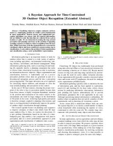
Consensus seeking formations of vehicles implies disciplined motion of several rigid vehicles (e.g spacecraft, unmanned aircraft, robotic vehicles etc) maintaining a desired geometric formation shape and geometry. Formation control is an important area of research not only for air and space vehicles but also for ground and under water vehicles. The applications of formations are numerous as with formations of spacecraft for unprecedented image resolution for astronomy and surveillance [1, 2], modeling of environment, surveillance and rescue missions in military applications, monitoring of forests and agricultural lands, healthcare applications, collaborative information processing, energy saving from vortex forces [3] and fuel efficiency via induced drag reduction [4]. Spacecraft formations have also been envisioned for distributed sensing for gravitational field mapping, atmospheric data sampling, co-observations (i.e, near-simultaneous observations of the same science target by instruments on multiple platforms), and synthetic radio-frequency and radar apertures. Formation flying can be used for airborne refueling and quick deployment of troops and vehicles. [5] looks at the problems related to formations of a number of small, low cost structures instead of one big instrument. Formations can be established in several ways that include leader-follower, behavioral method and virtual structures [1]. In leader-following formation, there is one leader and all the other vehicles follow the leader. In the behavioral method, a prescribed behavior is set for all the vehicles in the formation for example trajectory, neighbor tracking, collision and obstacle avoidance and formation keeping. In virtual structure approach, entire formation is treated as a single, virtual structure [6]. In this thesis we deal with the attitude (orientation) synchronization and tracking of a formation of rigid bodies under communication constraints which helps in maintaining the formation geometry. We develop the formation control [1, 3, 4, 7] using the theory of constraint forces to build formations from arbitrary initial conditions of the rigid bodies in formation. We develop general non-linear equations of motion of rigid bodies [8, 9] in a formation using the Euler-Lagrange Method [1, 2, 10]. 1

2

(a)

(b)

Figure 1.1. (a) Formation of Spacecraft and (b) Formation of Aircraft.

The formation is maintained due to the constraints acting between the rigid bodies which in the present context serves like an information exchange among the units in the formation. Communication [11] between these units helps in maintaining the formation; loss of which can make the overall formation unstable and could annihilate the formation as a consequence. For a coordinated team of multi-agents, the concept of graph theory has been shown to be very useful for inter-communication between the agents in recent years. Information consensus strategies based on graph theory for multiple vehicle control has been extensively addressed in [12]. Active constraints help in the local interactions between the units of this system [13]. Constraint forces [14] also determine the total force required on each rigid body to maintain the formation. To keep the formations intact, we develop a control law that is derived from a Baumgarte [1] like stabilization procedure. Similar work was done in [1, 7, 10] wherein constraints are stabilized via a proportional-derivative structure. We then show the attitude synchronization and tracking of this formation system similar to that in [2, 10]. Decentralized control approaches for formations are discussed in [15]. Decentralized [6, 11] information consensus requires only local neighbor-to-neighbor information exchange among the vehicles. The basic idea in this type of consensus is that each vehicle updates its information state based on the information states of its local neighbors so that the final information states of the total system converge to a common consensus value. Consensus problems have been applied in the context of formation control, self-alignment, flocking and network dynamics systems [16]. The problem of

3 desired reference state tracking is discussed in [10, 12]. In [17], invertibility of input-output maps and control system design for non-linear formation flying were considered.

(a)

(b)

Figure 1.2. (a) Robot Formation and (b) Constellation (Formation of Celestial bodies).

Several studies have addressed coordination control of multiple mobile robots (see [18] and references therein). Potential field approach is a popular approach to achieve coordination of multiple vehicles and shape the dynamics of the formation. Coordinated control using potential functions can be found in [19, 20, 21, 22, 23]. The basic idea in these studies is to create an energy-like function (potential function) to enforce position constraints between vehicles and use the negative gradient of the potential function as a restoring force on each vehicle to achieve coordination. The constrained dynamical approach in this thesis utilizes this basic idea to set up the control laws.

1.2

Problem Definition and Motivation

Motivated by developments in technology, the requirements of efficiency and quality in production have resulted in complex and integrated systems. The use of multi composed systems is spreading widely. Many multi composed systems work either under cooperative [18, 21] or coordinated schemes. Examples of such systems are abundant in nature (constellations), biological systems

4 (fish swarms, birds flock as shown in figure 1.3) and artificial machines (aircraft, spacecraft formation, multiple robots). Inspired by these systems and lured by its advantages, man has started mimicking such systems. Man made distributed systems are now being used to achieve efficiency and time and cost reduction. For example, formation of satellites as shown in figure 1.1(a), robots formation as shown in figure 1.2(a), marine craft formation, airplane formation etc [5, 13, 24]. However, many technical challenges must be addressed before controlled formation could be realized. For instance, it requires extensive technology development for precise attitude maintenance, controlled formation under external disturbances, tracking etc which requires that we need to address problems like synchronization, consensus, stability and tracking in general of these formation.

(a)

(b)

Figure 1.3. (a) Birds Flock and (b) School of fish.

Hence, synchronization [25] and consensus [12, 26, 27] of such systems is very important and has been studied since many years but has only recently caught much attention. The main contribution of this research is the development of the control algorithm for multiple rigid bodies using constraint forces that simultaneously achieve and maintain a given formation together with tracking [28]. For a large interconnected system with arbitrary connection topologies, the synthesis of a constraint potential is non-trivial. We solve this by exploiting the connection topology and synthesizing a potential energy function based on the graph Laplacian for this interconnected system [10, 24]. Once chosen, this still poses an additional difficulty of synthesizing the constraint Jacobians as re-deriving the Jacobian each time for a different connection topology is tedious. We address this issue by numerically synthesizing the Jacobian. Thus the framework only

5 needs to know the connection topology and the control laws are derived accordingly. In the present research, several candidate scenarios are evaluated such as tracking and finally unaided consensus. For detailed descriptions of these scenarios also see [12, 26, 27]. The problems related to synchronization, consensus and tracking are addressed using the stabilized constraint dynamics approach and are discussed in detail in Chapter 4. Another problem addressed in this research is the synchronization, consensus and tracking under unknown external disturbance. An adaptive control algorithm [29] is adopted to solve for an estimate of unknown disturbance through Lyapunov method [30, 31, 32] and a feed forward term is added to the external torque required to stabilize this disturbed system. Various cases (N-spacecraft formation, N-pendulum formation and N 2-link robotic manipulator) have been studied to test these techniques. These systems are simulated for various topologies of the rigid bodies and the results are obtained using simulations developed in the MATLAB environment.

CHAPTER 2 SYNCHRONIZATION OF MULTIPLE OSCILLATORS This chapter discusses the N-pendulum formation system as a motivating example. We start by discussing the Euler-Lagrange equations. Next, we derive the mathematical model (equations of motion) of a 2-pendulum formation. In this case a spring and a damper between the pendulums serve to model communication. The spring helps in the exchange of information between pendulums and damper helps in damping the motion of the system and stabilizing the system. Following this, we generalize the equations of motion for an N-pendulum formation. We proceed by establishing the stability of this formation using Lyapunov’s stability method. Finally, we simulate a 4-pendulum system for different sets of springs and dampers in MATLAB and verify the stability, synchronization and consensus using these simulations.

2.1

Euler-Lagrange Method

Euler-Lagrange method is an energy based method that can be used to derive the governing equations of motion of a dynamical system. In classical mechanics, we define the Lagrangian as the difference between the kinetic energy, T and the potential energy, U of a dynamical system. L=T −U

(2.1)

If we know the Lagrangian of a system, we can easily derive the equations of motion of that particular system by using the Euler-Lagrange equations given by, d dt

∂L ∂ q˙i

−

X ∂L = τi , i = 1, 2, . . . , N ∂qi

where qi is the generalized coordinate of the ith body in the system and

(2.2) P

τi is the sum of the

generalized external forces acting on the system. The Lagrangian formulation helps in deriving the equations of motion (EOM) of many complex systems which can otherwise be difficult to deal with using the Newton’s II law. This method is derived from the action principle which has applications to other fields like quantum mechanics etc. This formulation is advantageous as it is a generalized method which can be used to derive 6

7 EOM of complex systems using any coordinate system convenient to the user. EOM derived using this method are invariant under symmetry if the Lagrangian of that system is invariant.

2.2

Equations of Motion for a constrained 2-Pendulum system

Consider 2 pendulums under constraints, i.e a spring and a damper connecting the two center of masses of the pendulums. The constraint here models the information exchange between the pendulums and the damper helps in damping the motion of this system. We consider 2 pendulums having massless rods of lengths li and masses of bobs as mi , when disturbed from their equilibrium position (i.e vertical axis) makes angles θi where i = 1, 2.

Figure 2.1. 2-pendulum system.

ci and ki are the damping coefficient and the spring constant of damper and spring respectively of this system; a is the upstretched length of the spring; g is the acceleration due to gravity and is equal to 9.8m/s2 . For a system of N-pendulums in general, there are (N −1) springs and dampers in the system. Then, T =

N X 1 i=1

U=

N X i=1

2

mi li2 θ˙i2

mi ghi +

N −1 X i=1

1 ki ∆ri2 2

(2.3)

(2.4)

8 where hi = li (1 − cos θi )

(2.5)

gives the change in the height of the pendulums. ∆~ri = ∆xiî + ∆yi ˆj

(2.6)

is the displacement of the pendulums, where î and ˆj are the unit vectors in x and y direction. Also, ∆xi = l(i+1) sin θ(i+1) − li sin θi

(2.7)

∆yi = l(i+1) cos θ(i+1) − li cos θi where ∆x and ∆y is the displacement of the center of mass in x and y direction. Now, ∆r2

=

∆~r.∆~r

= l12 + l22 − 2l1 l2 cos (θ2 − θ1 )

(2.8) (2.9)

Differentiating equation (2.6), ∆r˙i = (l(i+1) cos θ(i+1) θ˙(i+1) − li cos θi θ˙i )î + (−l(i+1) sin θ(i+1) θ˙(i+1) + li sin θi θ˙i )ˆj

(2.10)

Lagrangian is given by: L=T −U Euler-Lagrange equations are given by: d ∂L ∂L ∂R X − = Qθi + dt ∂ θ˙i ∂θi ∂ θ˙i P where Qθi are the external forces acting on the 2-pendulum system. And, R

= =

1 ˙i ci ∆~r˙i ∆~r 2 1 2 ˙2 c(l θ + l12 θ˙12 − 2l2 l1 θ˙2 θ˙1 cos(θ2 − θ1 )) 2 2 2

(2.11)

(2.12)

(2.13) (2.14)

is the Rayleigh dissipation due to the damper involved in the 2-pendulum system. Substituting the values of L and R in the Euler-Lagrange equations and rearranging them gives the final equations of motion for this 2-pendulum system as, g kl2 c θ¨1 = − sin θ1 + sin (θ2 − θ1 ) − (l1 θ˙1 − l2 θ˙2 cos(θ2 − θ1 )) l1 m 1 l1 m1 l1

(2.15)

kl1 c g sin (θ2 − θ1 ) − (l2 θ˙2 − l1 θ˙1 cos(θ2 − θ1 )) θ¨2 = − sin θ2 − l2 m 2 l2 m2 l2

(2.16)

9 2.3

EOM for the Generalized N-Pendulum system

Following the same method of calculating the kinetic energy, potential energy and the Lagrangian of a generalized N-pendulum system, then using Euler -Lagrange equations we find the generalized equations of motion of the N-pendulum system which can also be found similarly by observing the pattern in the 2-pendulum system. The generalized N-pendulum system equations of motion are summarized below.

Figure 2.2. N-pendulum system.

For 1st pendulum: g k1 l2 c1 θ¨1 = − sin θ1 + sin (θ2 − θ1 ) − (l1 θ˙1 − l2 θ˙2 cos(θ2 − θ1 )) l1 m 1 l1 m1 l1

(2.17)

For i = 2 → (N − 1) pendulums: k(i−1) l(i−1) ki l(i+1) c(i−1) ˙ g sin (θi − θ(i−1) ) + sin (θ(i+1) − θi ) − (li θi θï = − sin θi − li mi li mi li mi li ci −l(i−1) θ˙(i−1) cos(θi − θ(i−1) )) − (li θ˙i − l(i+1) θ˙(i+1) cos(θ(i+1) − θi )) mi li

(2.18)

For N th pendulum: k(N −1) l(N −1) c(N −1) g θ¨N = − sin θN − sin (θN − θ(N −1) ) − (lN θ˙N − l(N −1) θ˙(N −1) cos(θN − θ(N −1) )) lN mN lN mN lN (2.19)

10 2.4

Stability of the N-Pendulum system

In this section, we prove analytically that the N-pendulum system can be stabilized by least number of dampers placed between any two pendulums in an N-pendulum system. Start by writing the kinetic energy of this system as: T =

N X 1 i=1

2

2 mi l12 θ˙i

(2.20)

Also, the potential energy of this system is as follows, U=

N X

mi gli (1−cos θi )+

N −1 X

i=1

i=1

1 ki [(l(i+1) sin θ(i+1) −li sin θi )2 +(l(i+1) cos θ(i+1) −li cos θi )2 ] (2.21) 2

Formulating the Hamiltonian or the total energy of this system as, T otalEnergy : V = T + U

(2.22)

The above is also a suitable Lyapunov function candidate. Differentiating the Lyapunov function candidate with respect to time as, N N −1 X X dV = (mi li2 θ˙i θï + mi gli sin θi θ˙i ) + ki [(l(i+1) sin θ(i+1) − li sin θi )(l(i+1) cos θ(i+1) θ˙(i+1) − li cos θi θ˙i ) dt i=1 i=1

−(l(i+1) cos θ(i+1) − li cos θi )(l(i+1) sin θ(i+1) θ˙(i+1) − li sin θi θ˙i )] (2.23) Substituting the values of θï from equations (2.17), (2.18) and (2.19) in the above (2.23) and rearranging the terms gives, N −1 X dV =− ci [(l(i+1) cos θ(i+1) θ˙(i+1) − li cos θi θ˙i )2 + (−l(i+1) sin θ(i+1) θ˙(i+1) + li sin θi θ˙i )2 ] (2.24) dt i=1

or dV = −2R dt

(2.25)

where R=

N −1 1 X ˙ i) (ci ∆~r˙ i ∆~r 2 i=1

(2.26)

From equation (2.24), we see that the change in the total energy is dependent on θi , θ˙i and li . Thus the rate at which this system stabilizes depends on the number of dampers in the system. When there are no dampers in the N-pendulum system, the system remains bounded but does not converge.

11 Now, to prove the stability of the N-pendulum formation system, rewrite equation (2.24) as: V˙ = −

N −1 X

ci (T erm1 + T erm2)

(2.27)

i=1

where T erm1 = (li cos θi θ˙i − l(i−1) cos θ(i−1) θ˙(i−1) )2

(2.28)

T erm2 = (−li sin θi θ˙i + l(i−1) sin θ(i−1) θ˙(i−1) )2

(2.29)

and

We see that equations (2.28) and (2.29) are positive for all values of li and θi , which makes equation (2.27) negative definite. From Lyapunov’s stability theorem [8] which states, Theorem: If a scalar function V (x, t) satisfies the following conditions: 1. V (x, t) is positive definite (that is, lower bounded). 2. V˙ (x, t) is negative semi-definite. 3. V˙ (x, t) is uniformly continuous in time. 4. V˙ (x, t) → 0 as t → ∞ we conclude that the system in equations (2.17)-(2.19) with V (x, t) in equation (2.22) is asymptotic stable (AS).

2.5

Simulation Results

We simulate the equations of motion of the 4-pendulum system in MATLAB and we plot the results showing the variation of the angles θi with time and the phase plots with different values of ci (damping coefficient) and ki (spring constant). In this system there are 3 springs and 3 dampers.

2.5.1

Case 1: Damping coefficients (c1 , c2 , c3 ) = (1, 1, 1) In this case, initial condition of orientations and angular velocities are (θ1 , θ2 , θ3 , θ4 , θ˙1 , θ˙2 , θ˙3 , θ˙4 ) =

(1, 1, 1, 1, 1, 1, 1, 1), masses of the bobs are (m1 , m2 , m3 , m4 ) = (1, 1, 1, 1) and lengths of pendulums are (l1 , l2 , l3 , l4 ) = (1, 1, 1, 1). The results are shown in figure 2.3. We see that all the pendulums synchronize and stabilize.

2.5.2

Case 2: Limited number of dampers as (c1 , c2 , c3 ) = (1, 0, 0) In this case, initial masses of bobs are (m1 , m2 , m3 , m4 ) = (1, 1, 1, 1), lengths of pendulums

are (l1 , l2 , l3 , l4 ) = (1, 1, 1, 1), spring constants are (k1 , k2 , k3 ) = (1, 1, 1) and initial conditions of

12

Figure 2.3. 4-pendulum system with (c1 , c2 , c3 ) = (1, 1, 1). orientations and angular velocities are (θ1 , θ2 , θ3 , θ4 , θ˙1 , θ˙2 , θ˙3 , θ˙4 ) = (1, 1, 1, 1, 1, 1, 1, 1). The results are shown in figure 2.4. In this case, the motion is damped slowly as there is only one damper.

Figure 2.4. 4-pendulum system with (c1 , c2 , c3 ) = (1, 0, 0).

CHAPTER 3 FORMATION OF N 2-LINK ROBOT MANIPULATORS This chapter discusses the formation control of N 2-link robotic manipulators. As was done in the previous chapter, we first develop the EOM of a 2-link robotic manipulator using the EulerLagrange method. The next section derives the generalized EOM for N 2-link robotic manipulators.

3.1

2-link Robotic Manipulator

Figure 3.1. A 2-link robotic manipulator.

Consider a 2-link robotic manipulator, i.e it has 2 degrees of freedom. The manipulator consists of 2-rigid links where l1 and l2 are the lengths of it’s first and second arms. m1 and m2 are the distributed masses of the two arms of the robotic manipulator, that is, the center of mass for

13

14 each link is at the center of each arm. The moments of inertia of the two arms are I1 and I2 . Now, from the figure 3.1, 1 xD = l1 cos θ1 + l2 cos (θ1 + θ2 ) 2 1 yD = l1 sin θ1 + l2 sin (θ1 + θ2 ) 2 1 xC = l1 cos θ1 2 1 yC = l1 sin θ1 2

(3.1)

where xD , yD , xC and yC are the positions of the points D and C. Differentiating equation (3.1) gives the velocity of the center of masses, i.e C and D. 1 x˙ D = −l1 sin θ1 θ˙1 − l2 sin (θ1 + θ2 )(θ˙1 + θ˙2 ) 2 1 y˙ D = l1 cos θ1 θ˙1 + l2 cos (θ1 + θ2 )(θ˙1 + θ˙2 ) 2 1 x˙ C = − l1 sin θ1 θ˙1 2 1 y˙ C = l1 cos θ1 θ˙1 2

(3.2)

The total velocity of the center of mass D is given by 2 vD

2 = x˙ 2D + y˙ D (3.3) 2 2 1 1 = −l1 sin θ1 θ˙1 − l2 sin (θ1 + θ2 )(θ˙1 + θ˙2 ) + l1 cos θ1 θ˙1 + l2 cos (θ1 + θ2 )(θ˙1 + θ˙2 )(3.4) 2 2 1 = l12 θ˙12 + l22 (θ˙1 + θ˙2 )2 + l1 l2 θ˙1 (θ˙1 + θ˙2 ) [sin θ1 sin (θ1 + θ2 ) + cos θ1 cos (θ1 + θ2 )] (3.5) 2 1 = l12 θ˙12 + l22 (θ˙1 + θ˙2 )2 + l1 l2 θ˙1 (θ˙1 + θ˙2 ) cos θ2 (3.6) 2

The total kinetic energy is

1 ˙2 1 1 2 2 ˙ ˙ IA θ1 + ID (θ1 + θ2 ) + m2 VD T = 2 2 2 where, IA = 13 m1 l12 and ID =

1 2 12 m2 l2

(3.7)

are the moment of inertia of arms 1 and 2. Then,

1 1 1 1 1 2 2 2 2 2 ˙ ˙ ˙ T = m1 l1 θ1 + m2 l2 (θ1 + θ2 ) + m2 VD 2 3 2 12 2

(3.8)

Substituting equation (3.3) in (3.8) and regrouping the similar terms T = θ˙12

1 1 1 1 1 1 1 m1 l12 + m2 l22 + m2 l12 + m2 l1 l2 cos θ1 +θ˙22 m2 l22 +θ˙1 θ˙2 m2 l22 + m2 l1 l2 cos θ2 6 6 2 2 6 3 2 (3.9)

15 The total potential energy of this system is the sum of the potential energies of the two links. l1 l2 U = m1 g sin θ1 + m2 g l1 sin θ1 + sin (θ1 + θ2 ) 2 2

(3.10)

where g is acceleration due to gravity. Now, the Lagrangian for the 2-link robot arm is given by the difference between the total kinetic energy and potential energy. (3.11)

L=T −U

Substituting the values of T and U from equations (3.9) and (3.10) in (3.11) and solve to get 1 1 1 1 1 1 1 2 2 2 2 2 2 2 ˙ ˙ ˙ ˙ L = θ1 m1 l1 + m2 l2 + m2 l1 + m2 l1 l2 cos θ2 + θ2 m2 l2 + θ1 θ2 m2 l2 + m2 l1 l2 cos θ2 6 6 2 2 6 3 2 l1 l2 −m1 g sin θ1 − m2 g l1 sin θ1 + sin θ1 + θ2 2 2 (3.12) The Euler-Lagrange equations are given by: d dt

∂L ∂ θ˙ i

−

∂L = τi ∂ θ˙ i

(3.13)

where i = 1, 2 in this case. τi is the sum of all the generalized external torques. Using equation (3.12) into (3.13), we get the equations of motion of a 2-link robotic arm as, 1 1 1 1 τ1 = m1 l12 + m2 l12 + m2 l22 + m2 l1 l2 cos θ2 θ¨1 + m2 l22 + m2 l1 l2 cos θ2 θ¨2 − (m2 l1 l2 sin θ2 ) θ˙1 θ˙2 3 3 3 2 1 1 1 m2 l1 l2 sin θ2 θ˙22 + m1 + m2 gl1 cos θ1 + m2 gl2 cos (θ1 + θ2 ) − 2 2 2 (3.14) τ2 =

1 1 1 1 1 m2 l22 + m2 l1 l2 cos θ2 θ¨1 + m2 l22 θ¨2 + m2 l1 l2 sin θ2 θ˙12 + m2 gl2 cos (θ1 + θ2 ) 3 2 3 2 2 (3.15)

We can write equations (3.14) and (3.15) in generalized matrix form as, 

τ1

 τ2





=

h11

h12

h21

h22



θ¨1



θ¨2





+

f11 θ˙1 + e11 θ˙2

f12 θ˙2 + e12 θ˙2



θ˙1

f21 θ˙1 + e21 θ˙2

f22 θ˙2 + e22 θ˙1



θ˙2





+

g11

 

g21

The above generalized matrix form can be rewritten in compact form as, ¯ i (θi , θ˙i )θ˙i + Gi (θi ), τi = Hi (θi )θï + C

i = 1, 2

(3.16)

16 where h11 =

1 1 1 1 m1 l12 + m2 l12 + m2 l22 + m2 l1 l2 cos θ2 , h12 = m2 l22 + m2 l1 l2 cos θ2 , 3 3 3 2 1 1 1 h21 = m2 l22 + m2 l1 l2 cos θ2 , h22 = m2 l22 , 3 2 3

f12 = −

1 m2 l1 l2 sin θ2 , f21 = 2

f11 = 0, f22 = 0, 1 m2 l1 l2 sin θ2 , 2

(3.17)

e11 = − (m2 l1 l2 sin θ2 ) , e12 = 0, e21 = 0, e22 = 0, g11 =

1 1 m1 + m2 gl1 cos θ1 + m2 gl2 cos (θ1 + θ2 ), 2 2 3.2

g21 =

1 m2 gl2 cos (θ1 + θ2 ) 2

EOM of N 2-link Robotic Manipulator

Figure 3.2. Three 2-link robotic manipulator formation.

In this section, we consider N 2-link robotic manipulators. The generalized equations of motion of N 2-link robotic manipulators is written in compact form as ¯ i (θi , θ˙i )θ˙i + Gi (θi ) τi = Hi (θi )θï + C where i = 1, 2, 3 . . . N .

(3.18)

17 Dropping the index i and writing the equation (3.18) for N 2-link robotic manipulators as, ¯ θ˙ + G τ = Hθ¨ + C where







 H1  H=      G=  

..

. HN

 G1 .. .

¯  C1     , C ¯ =     

     , τ =    

(3.19)

 τ1 .. .

 ..

.



     and θ =     

¯N C  θ1  ..  .    θN

    

τN GN Note, that each θi = θi1 , θi2 is a two component attitude vector.

In order for this system to maintain a prescribed formation, communication constraints should be developed which enforce synchronization, consensus and tracking. The generalized communication constraints are developed in the next chapter using the graph theory.

CHAPTER 4 CONSTRAINED DYNAMICS FORMULATION To maintain the formation of N -rigid bodies (spacecraft, aircraft, pendulums, robots etc), constraints could be employed to achieve the formation. These constraints aid in the consensus and synchronization of the attitude of the rigid bodies depending upon how these are enforced. In this chapter, we first develop the graph theory background needed in formulating the communication constraints. We then develop the generalized constraints required for maintaining the N-rigid bodies in formation. We then develop the N 2-link robotic manipulator EOM with the constraint dynamics. Once the EOM of the formation under constraints are developed, a Baumgarte stabilization technique is applied to stabilize this formation. Finally, the formation is simulated in MATLAB for various communication topologies and the cases of synchronization, tracking and consensus are shown.

4.1

Graph Theory Background

A graph is a pair G = (V, E) where V is a finite nonempty set of nodes or vertices V = {v1 , v2 , v3 , . . . , vN } and a set of edges or arcs E ⊆ V × V. We assume vi , vi 6⊆ E, ∀ i, i.e no self loops. Edge eij = (vi , vj ) is said to be outgoing with respect to node vi and incoming with respect to vj . If every possible arc exists, the graph is said to be complete. If (vi , vj ) ⊂ E ⇒ (vj , vi ) ⊂ E, ∀ i, j the graph is said to be undirected, otherwise it is directed and is termed as digraph. The edges are represented by an adjacency matrix

Figure 4.1. Graph showing node and edge.

18

19 A = [aij ]

(4.1)

with aij = 1 if (vj , vi ) ⊂ E and aij = 0 otherwise. Also, aii = 0. For an undirected graph A is symmetric. The weighted adjacency matrix is given by Aw = ìj [aij ]

(4.2)

where ìj are the weights of each edge in the graph. The in-degree of vi is the number of edges having vi as a head i.e. ith row sum di = The out-degree of a node vi is the number of edges having vi as a tail, i.e. ith

P aij . j P column sum do = aji . j

If the in-degree equals the out-degree for all nodes v ∈ V, the graph is said to be balanced. The valency matrix of the graph is a diagonal matrix given as,   N X D = diag  aij 

(4.3)

j=1

The weighted valency matrix is given by:  Dw = diag 

N X

 ìj [aij ]

(4.4)

j=1

Now the structure of the graph is given by the Laplacian matrix i.e. (4.5)

L=D−A and the weighted Laplacian matrix is given by: Lw = Dw − Aw

(4.6)

Example: An example of a graph showing how to formulate the Laplacian is explained below for the connection topology explained below. In this case, a desired (reference node)rigid body is connected to rigid body 1 which is connected to 2 and 2 to 3. Then,     σ1   A=  σ2    σ3  σd

σ1

σ2

σ3

0

0

0

1

0

0

0

1

0

0

0

0

σd



  1    0     0   0

20

Figure 4.2. Graph topology. The rows of A are given by the in degree of that particular node. For example, σ1 is the in degree of σ2 , σ2 is the in degree of σ3 and σd is the in degree of σ1 . Then, 

 1   0  D=  0   0

0

0

1

0

0

1

0

0

 0   0    0    0

and L = D − A. Hence, 

 1   −1  L=  0   0 4.2

0 1 −1 0

 0 −1   0 0    1 0    0 0

Development of Generalized Constraints for an N-Rigid bodies system

Consider an N rigid bodies system whose attitude is given by qi . q = {q1 , q2 , . . . , qN } represents the collection of the attitudes of N rigid bodies with respect to the inertial frame. To ˜ which is given by: develop the constraints, consider a mapping from q 7→ y(L) y = L˜ q

(4.7)

where L˜ ∈ Rj×N has number of rows equal to j and number of columns equal to the total number of rigid bodies in the system i.e N . Also, j = total number of rigid bodies having an out-degree with out-degree ≥ 1. y ∈ Rj×1 is a vector with j rows and 1 column.

21 Now, the constraints (akin to directional communication between a body and others in the formation), are represented as scalar potential functions given by: C(q1 , q2 . . . qN )

=

yT y

(4.8)

=

(L˜ q)T L˜ q

(4.9)

=

˜ qT (L˜T L)q

(4.10)

L˜ is also called the error Laplacian and is derived from L. The above form of constraint potential ensures the attitude consensus and tracking. For the attitude tracking consensus problem, when all the rigid bodies track a desired reference attitude, the attitude vector of the system then becomes q = {q1 , q2 , . . . , qN , qd } where q ∈ R(N +Nd )×1 with additional reference attitudes included. Nd are the total number of desired reference attitude vectors. For such a case, L˜ will be constructed with this new q attitude vector. Using the connection topology as given in example shown in figure 4.2, we develop the constraints as, 

 1   −1  L˜ q =   0   0

0 1 −1 0

 0 −1     0 0     1 0    0 0

 q1   q2    q3    qd

Then, 

 q − q d   1    q2 − q1    L˜ q =    q −q   3 2    0 Finally, 

C=

q1 − qd

q2 − q1

q3 − q2

 q1 − qd   q2 − q1  0   q −q  3 2  0

        

giving C = (q1 − qd )2 + (q2 − q1 )2 + (q3 − q2 )2

(4.11)

22 4.3

Constrained EOM formulation for N 2-link robotic manipulator system

Using the above formulated constraints and applying it to N 2-link robotic manipulator system, we find that the above constraints for this case is written as, C(θ1 , θ2 . . . θN )

= yT y

(4.12)

(L˜ θ)T L˜ θ

(4.13)

˜ = θT (L˜T L)θ

(4.14)

=

where, attitude of this system is expressed as θ = {θ1 , θ2 , . . . , θN }. Here, each θi = θi1 , θi2

is a two component attitude vector. With the constraint potentials formulated, the Lagrangian is modified as follows, Lm = L + ΛT C

(4.15)

where Λ is the vector of Lagrange Multipliers of this system of N 2-link robotic manipulators given T

T

by Λ = (λ1 , λ2 , . . . , λM ) and C = (C1 , C2 , . . . , CM ) is the vector of constraint potentials. The modified Euler-Lagrange equations for this system under constraints is given by: T ∂L ∂Ci (θ) d ∂L − + Λ = τi (4.16) dt ∂ θ˙i ∂θi ∂θi where τi is the vector of generalized external torques acting on the ith body. Denoting Wi as the h i ∂Cj (θ) Jacobian of the constraints for the ith body, i.e.Wi = , the equations of motion for this ∂θi constrained system is obtained as, 2

Hj θ¨j + Fj θ˙j + Gj (θ˙i , θ˙i+1 )j + Ej = (τj − Wj T Λ)

(4.17)

where, equation (4.17) can be rewritten as, h i θ¨j = Hj −1 (τj − Wj T Λ) − Fj θ˙j2 − Gj (θ˙i , θ˙i+1 )j − Ej

(4.18)

Dropping the arguments in equation (4.17) for the sake of brevity, we get Hθ¨ + Fθ˙2 + G(θ˙i θ˙i+1 ) + E = (τ − WT Λ) where,    W=  

 W1 .. . WN

    

(4.19)

23 Differentiating the constraints C with respect to time yields, C˙ = Wθ˙ = 0

(4.20)

Upon differentiation of equation (4.20) with respect to time, ˙ θ˙ + Wθ¨ = 0 C¨ = W

(4.21)

Substituting the value of θ¨ from equation (4.19) into (4.21) we get i h ˙ θ˙ + W H−1 τ − WT Λ − Fθ˙2 − G(θ˙i , θ˙i+1 ) − E = 0 W

(4.22)

The above can be trivially solved for Λ, i −1 h ˙ θ˙ Λ = WH−1 WT WH−1 τ − Fθ˙2 − G(θ˙i θ˙i+1 ) − E + W

(4.23)

where WH−1 WT is a square matrix. Substituting Λ back in equation (4.19) yields the constrained equations of motion.

4.4

Baumgarte Stabilization of Constraints

The control torque required to enforce the formation constraints is derived using Baumgarte stabilization technique. Equation (4.21) is modified to include stabilization terms, i.e. C¨ = −Kd C˙ − Kp C

(4.24)

where Kp and Kd are appropriately chosen positive definite matrix gains for the proportional and derivative (PD) terms. Then, i −1 h ˙ θ˙ + Kp C + Kd C˙ Λ = WH−1 WT WH−1 τ − Fθ˙2 − G(θ˙i , θ˙i+1 ) − E + W

(4.25)

It can be easily shown that the Λ obtained from equation (4.25), when substituted into equation (4.19) ensures that the N 2-link robotic manipulator formation system is asymptotically stable. If we choose value of the control torque given by i −1 h ˙ θ˙ − WH−1 (Fθ˙2 + G(θ˙i , θ˙i+1 ) + E) + Kp C + Kd C˙ τ = −WT WH−1 WT W

(4.26)

This value of external control torque τ ensures that Λ = 0 and ensures that C → 0 thus leading to synchronization and asymptotic stability of the formation.

24 Lemma 1: The choice of the external torque as

i −1 h ˙ θ˙ − WH−1 (Fθ˙2 + G(θ˙i , θ˙i+1 ) + E) + Kp C + Kd C˙ τ = −WT WH−1 WT W ensures C(t) → 0 as t → ∞. Proof: For the above value of control torque given by τ , we can write i h ¨ θ˙2 +G(θ˙i , θ˙i+1 )+E = −WT WH−1 WT −1 W ˙ θ˙ − WH−1 (Fθ˙2 + G(θ˙i , θ˙i+1 ) + E) + Kp C + Kd C˙ Hθ+F (4.27) Pre multiplying both sides of equation (4.27) by WH−1 gives h i ˙ θ˙ − WH−1 (Fθ˙2 + G(θ˙i , θ˙i+1 ) + E) + Kp C + Kd C˙ WH−1 [Hθ¨ + Fθ˙2 + G(θ˙i , θ˙i+1 ) + E] = − W (4.28) Simplifying equation (4.28) gives ˙ θ˙ + Kp C + Kd C˙ = 0 Wθ¨ + W

(4.29)

Using equation (4.20) in above, we get C¨ + Kp C + Kd C˙ = 0

(4.30)

Choosing appropriate values of Kp , Kd > 0, we see C → 0 as t → ∞ from equation (4.24).

4.5

MATLAB Results

The simulation results in this case corresponds to different scenarios. (m1 , m2 ) = (10, 5), (m3 , m4 ) = (10, 5) and (m5 , m6 ) = (10, 5) are the initial conditions of the masses of the arms of 1st , 2nd , 3rd and the reference robots respectively. (l1 , l2 ) = (5, 2), (l3 , l4 ) = (5, 2), (l5 , l6 ) = (5, 2) and (ld1 , ld2 ) = (5, 2) are the initial conditions of lengths of the 1st , 2nd , 3rd and the reference robotic arms respectively.

4.5.1

Connection Topology 1 In this case the connection topology (CT1) is considered as shown in figure 4.3 where desired

reference robot is connected to 1. 1 is connected to 2 and 2 to 3.

25

Figure 4.3. Case 1 Topology.



 0   1  A1 =   0   0 

 1   0  D1 =   0   0

0

0

0

0

1

0

0

0

0

0

1

0

0

1

0

0

 1   0    0    0  0   0    0    0

Now, L1 = D1 − A1 . Figure 4.4 show results corresponding to tracking performance for a constant desired attitude. Clearly, all the formation objectives are met and the three vehicles converge to a constant orientation. The initial conditions of the orientations of the robots are robot1 (θ) = (−0.2, 0.2), robot2 (θ) = (−0.1, 0.1), robot3 (θ) = (0.2, −0.2) and robotd (θ) = (0.2, 0.1). The initial conditions of the angular velocities of the robots are robot1 (ω) = (0, 0), robot2 (ω) = (0, 0), robot3 (ω) = (0, 0) and robotd (ω) = (0, 0). The PD gains are Kp = 10 and Kd = 80.

4.5.2

Connection Topology 2 In this case the connection topology (CT2) is considered as shown in figure 4.5 where the

reference robot is connected to robot 1 which is connected to 2, 2 to 3 and 3 to 1.

26

Figure 4.4. CT1: Tracking a constant orientation θd = (0.2, 0.1).




 0   1  A2 =   0   0 

 2   0  D2 =   0   0

0

1

0

0

1

0

0

0

0

0

1

0

0

1

0

0

 1   0    0    0  0   0    0    0

Now, L2 = D2 −A2 . Figure 4.6 show results corresponding to tracking performance for a constant desired attitude. All the 3 robots track the attitude of the desired vehicle and converge to a con-

27 stant orientation. The initial conditions of the orientations of the robots are robot1 (θ) = (−0.2, 0.2), robot2 (θ) = (−0.1, 0.1), robot3 (θ) = (0.2, −0.2) and robotd (θ) = (0.2, 0.1). The initial conditions of the angular velocities of the robots are robot1 (ω) = (0, 0), robot2 (ω) = (0, 0), robot3 (ω) = (0, 0) and robotd (ω) = (0, 0). The PD gains are Kp = 20 and Kd = 700.

Figure 4.6. CT2: Tracking a constant orientation θd = (0.2, 0.1).

4.5.3



In this case, the connection topology (CT3) is considered as shown in figure 4.7 where robot 1 is connected to 2, 2 to 3 and 3 to 1.

28  0 0 1      A3 =  1 0 0     0 1 0   1 0 0      D3 =  0 1 0     0 0 1 

Now, L3 = D3 − A3 . Figure 4.8 show results corresponding to consensus of the three 2-link robotic manipulators. All the three 2-link robotic manipulators should converge to the average of their initial values. The initial conditions of the orientations of the robots are robot1 (θ) = (−0.2, 0.2), robot2 (θ) = (−0.1, 0.1) and robot3 (θ) = (0.2, −0.2) . The initial conditions of the angular velocities of the robots are robot1 (ω) = (0, 0), robot2 (ω) = (0, 0) and robot3 (ω) = (0, 0). The PD gains are Kp = 20 and Kd = 500. In this case, we see that the consensus is not achieved. It is because this system is highly non-linear and for some unknown reasons, for only some sets of initial values we achieve average consensus in true sense. So, various values of initial conditions should be tried to show consensus results.

Figure 4.8. CT3: Average consensus of orientations.

4.5.4

Connection Topology 4 In this case, the connection topology (CT4) considered corresponds to where the desired

reference vehicle is connected to 1, 1 is connected to 2, 1 to 3 and 2 to 3 as shown in figure 4.9.

29




 0   1  A4 =   1   0 

 1   0  D4 =   0   0

0

0

0

0

1

0

0

0

0

0

1

0

0

2

0

0

 1   0    0    0  0   0    0    0

Now, L4 = D4 − A4 . Figure 4.10 show results corresponding to tracking performance for a constant desired attitude. All the 3 robots track the attitude of the desired vehicle and converge to a constant orientation. The initial conditions of the orientations of the robots are robot1 (θ) = (−0.3, 0.2), robot2 (θ) = (0.4, −0.2), robot3 (θ) = (−0.5, −0.7) and robotd (θ) = (−0.5, 0.3). The initial conditions of the angular velocities of the robots are robot1 (ω) = (0, 0), robot2 (ω) = (0, 0), robot3 (ω) = (0, 0) and robotd (ω) = (0, 0). The PD gains are Kp = 50 and Kd = 150.

4.5.5


reference vehicle is connected to 1, 1 is connected to 2, 2 to 1, 2 to 3 and 3 to 1 as shown in figure 4.11.

30

Figure 4.10. CT4: Tracking a constant orientation θd = (−0.5, 0.3).




 0   1  A5 =   0   0 

 3   0  D5 =   0   0

1

1

0

0

1

0

0

0

0

0

1

0

0

1

0

0

 1   0    0    0  0   0    0    0

Now, L5 = D5 − A5 . Figure 4.12 show results corresponding to tracking performance for a constant desired attitude. All the 3 robots track the attitude of the desired vehicle and converge

31 to a constant orientation. The initial conditions of the orientations of the robots are robot1 (θ) = (−0.3, 0.2), robot2 (θ) = (0.4, −0.2), robot3 (θ) = (−0.5, −0.7) and robotd (θ) = (−0.5, 0.3). The initial conditions of the angular velocities of the robots are robot1 (ω) = (0, 0), robot2 (ω) = (0, 0), robot3 (ω) = (0, 0) and robotd (ω) = (0, 0). The PD gains are Kp = 50 and Kd = 180.

Figure 4.12. CT5: Tracking a constant orientation θd = (−0.5, 0.3).

CHAPTER 5 SPACECRAFT ATTITUDE FORMATION This chapter discusses the spacecraft attitude formation problem. We make use of the Modified Rodrigues parameters (MRP) for describing the attitude of the spacecraft. The first section in this chapter discusses the Modified Rodrigues Parameters and their advantages. Next we develop the equations of motion of a single spacecraft followed by the N-spacecraft formation. We then incorporate the constraints as discussed in Chapter 4 along with the spacecraft dynamics using the modified Euler-Lagrange equations to get an N-spacecraft formation system. The constraints are then stabilized using the Baumgarte stabilization technique thus stabilizing the whole formation. Finally, this system is simulated in MATLAB for different topologies and the results are shown verifying stability, synchronization, consensus and tracking.

5.1

Modified Rodrigues Parameters

The parameters used to describe the attitude (orientation) [33] of a spacecraft (s/c) in this chapter are the Modified Rodrigues parameters (MRP). If eˆ and φ denote the principal axis and the principal angle [33] respectively, then the MRP has the advantage that the kinematics remains non singular for eigenaxis rotations up to 360o . Additionally, we have a minimum parameter representation. Alternate representations such as the euler angles (321) have a singularity at θ = ± π2 where θ is the pitch angle. If eˆ and φ denote the principal axis and the principal angle [33] respectively, then the quaternions are represented as 

 β o      β1       β   2    β3

32

33 where φ 2 φ β1 = eˆ1 sin 2 φ β2 = eˆ2 sin 2 φ β3 = eˆ3 sin 2 βo = cos

(5.1)

The quaternions are a 4 parameter set with the unit norm constraint as, βo2 + β12 + β22 + β32 = 1

(5.2)

Thus, while there is no singularity, they are a non-minimal set and are constrained.

5.1.1

Derivation of Modified Rodrigues Parameters The MRPs are constructed from quaternions as follows: β1 1 + βo β2 σ2 = 1 + βo β3 σ3 = 1 + βo σ1 =

Figure 5.1. Axis Angle Coordinate (http : //en.wikipedia.org/wiki).

(5.3)

34 So, φ 4 φ σ2 = eˆ2 tan 4 φ σ3 = eˆ3 tan 4

σ1 = eˆ1 tan

(5.4)

Thus, MRPs are 3-parameter coordinates (minimum parameters) with singularity at eigenaxis rotation of only 360o which is not a hindrance as the rigid body can perform all the maneuvers till 360o . Hence σi → ∞ when φ → 2π and when σi = 0, φ = 0.

5.2

Derivation of Equations of Motion of a Spacecraft

Consider a spacecraft whose attitude is expressed in terms of the Modified Rodrigues Parameters (MRP) [9]. Let σ1 , represent the orientation of the s/c with respect to the inertial frame. The Lagrangian approach [10, 1, 2] is employed to derive the governing equations of motion of this s/c. Note, σ1 = σ11 , σ12 , σ13 is the three component attitude vector. The rotational kinematics of the s/c can be represented as follows, (5.5)

σ˙ 1 = J1 (σ1 )ω1 where, 1 J1 (σ1 ) = 2

σ ˜1 + σ1 σ1

T

1 + σ1 T σ1 I3 − 2

(5.6)

where, I3 is a 3 × 3 identity matrix and σ ˜1 = [σ1 ×] is a skew-symmetric matrix given as,   3 2 σ1 −σ1   0   3 [σ1 ×] =  0 σ11   −σ1    σ12 −σ11 0 where, [9] ω1 is the angular velocity in the body fixed frame and M1 is the symmetric moment of inertia matrix of the s/c. Using equation (5.5), [34] the Lagrangian, L is expressed as L = T , where T is the system kinetic energy, i.e. L=

1 T σ˙ H1 (σ1 )σ˙ 1 2 1

(5.7)

where H1 (σ1 ) = J1 −T M1 J1 −1

(5.8)

35 The Euler-Lagrange equations to derive the dynamics of this system is given by: d ∂L ∂L − = τ1 dt ∂ σ˙ 1 ∂σ1

(5.9)

where, τ1 is the generalized external torque acting on the s/c. ¯ 1 (σ1 , σ˙ 1 )σ˙ 1 = τ1 H1 (σ1 )¨ σ1 + C

(5.10)

−1 ¯ 1 (σ1 , σ˙ 1 ) = J1 −T M1 J˙ −1 + J1 −T J1g where, C σ˙ 1 M1 J1 −1 . 1

5.3

Formulation of Equations of Motion of N-Spacecraft

For N spacecraft system [σ1 , σ2 , . . . , σN ] represents the orientation vector of this system. T σi = σi1 σi2 σi3 is the three component attitude vector. The rotational kinematics of the system of spacecraft is represented as follows, σ˙ i = Ji (σi )ωi ,

i = 1, 2, . . . , N

(5.11)

Implicit in the discussion here is the fact that the three component attitude vector is treated as a single node. Also, Ji (σi ) =

1 2

1 + σi T σi σ ˜i + σi σi T − I3 2

(5.12)

where, I3 is a 3 × 3 identity matrix and σ ˜i = [σi ×] is a skew-symmetric matrix such as,   3 2 0 σ −σ i i      3 1 [σi ×] =  −σi 0 σi     σi2 −σi1 0 where, ωi is the angular velocity in the body fixed frame and Mi is the symmetric moment of inertia matrix of the ith spacecraft. Using equation (5.11), the Lagrangian, L is written as L = T , where T is the system kinetic energy, i.e. N

1X T σ˙ Hi (σi )σ˙ i 2 i=1 i

(5.13)

Hi (σi ) = Ji −T Mi Ji −1

(5.14)

L= where

The Euler-Lagrange equations used for formulating the dynamics of this system is: d ∂L ∂L − = τi dt ∂ σ˙ i ∂σi

(5.15)

36 where, σ = {σ1 , σ2 , . . . , σN } and τi is the vector of generalized external torques acting on the ith s/c. The equations of motion of N-spacecraft without any external disturbances is as follows: ¯ i (σi , σ˙ i )σ˙ i = τi Hi (σi )¨ σi + C

(5.16)

−1 ¯ i (σi , σ˙ i ) = Ji −T Mi J˙ −1 + Ji −T Jig where, C σ˙ i Mi Ji −1 . i

5.4

Constrained Rotational Equations of Motion of N-Spacecraft

Using the generalized form of communication constraints developed in Chapter 4, we develop the EOM of the constrained formation of N-spacecraft in this section. The constraint potential for the spacecraft dynamics becomes: C(σ1 , σ2 . . . σN )

= yT y

(5.17)

(L˜ σ)T L˜ σ

(5.18)

˜ = σ T (L˜T L)σ

(5.19)

=

where L˜ is the error Laplacian, L is the Laplacian and σ = {σ1 , σ2 , . . . , σN }. Once the constraint potentials are set, use the same method as applied to N 2-link robotic manipulators, i.e augment the original Lagrangian by the constraints. Then using the modified Euler-Lagrange equations, formulate the constrained EOM of N-spacecraft formation given as, ¯ i (σi , σ˙ i )σ˙ i = (τi − Wi T Λ) Hi (σi )¨ σi + C

(5.20)

−1 ¯ i (σi , σ˙ i ) = Ji −T Mi J˙ −1 + Ji −T Jig where, C σ˙ i Mi Ji −1 . i ¯ i (., .) are dropped for the sake of brevity. Thus the generalized The arguments of Hi (.) and C constrained system of N spacecraft formation can be written as follows ¯ σ˙ = τ − WT Λ H¨ σ+C

(5.21)

where,   H1 (σ1 )  H(σ) =   

 ..

. HN (σN )



¯   C1 (σ1 , σ˙ 1 )    , C(σ, ¯ σ) ˙ =    

 ..

. ¯ N (σN , σ˙ N ) C

    

37 

   W(σ) =   

W1 (σ) .. . WN (σ)



     and τ =     

 τ1 .. . τN

    

Using the constraint dynamics from equations (4.20) and (4.21) and substituting the value of σ ¨ from Equation (5.21) into (4.21) we obtain ˙ σ˙ + W H−1 τ − WT Λ − C ¯ σ˙ = 0 W

(5.22)

i −1 h ˙ − WH−1 C ¯ σ˙ WH−1 τ + W Λ = WH−1 WT

(5.23)

Solving for Λ,

where WH−1 WT is a square matrix. Substituting Λ back in equation (5.21) yields the constrained equations of motion. The constraint dynamics are in-built in the spacecraft dynamics using Equations (4.20) and (5.9).

5.5

Baumgarte Stabilization of Constraints

Using the Baumgarte stabilization technique as explained in Chapter 4, using equation (4.24) we find Λ as Λ =

i i −1 h h ˙ − WH−1 C ¯ σ˙ + WH−1 WT −1 Kp C + Kd C˙ WH−1 WT WH−1 τ + W (5.24)

Λ obtained from equation (5.24), when substituted into equation (5.21) ensures that the N -spacecraft formation is asymptotically stable. If we choose value of the control law given by i −1 h ˙ − WH−1 C ¯ σ˙ + Kp C + Kd C˙ τ = −WT WH−1 WT W

(5.25)

it ensures that Λ = 0 and C → 0 which leads to synchronization and asymptotic stability of the formation. The proof of this can be shown in a similar way as shown in Chapter 4 using Lemma 1.

5.6

MATLAB Simulation Results

The simulation results are shown corresponding to the scenarios shown in Chapter 4. The moment of inertia of all the bodies are assumed to be identically equal which is

38  0   0    40

  40  M=  0  0 5.6.1

0 40 0


reference vehicle is connected to 1, 1 is connected to 2 and 2 to 3. Then, 

 0   1  A1 =   0   0

0

0

0

0

1

0

0

0



1   0    0    0

Figure 5.2 show results corresponding to tracking performance for a constant desired attitude. Clearly, all the formation objectives are met and the three vehicles converge to a constant orientation. The initial conditions of attitude are (σ1 , σ2 , σ3 , σd ) = (−0.2, 0.5, −0.4, 0.2) and angular velocities are (ω1 , ω2 , ω3 , ωd ) = (0, 0, 0, 0). The PD gains are Kp = 4 and Kd = 20.

Figure 5.2. CT1: Tracking a constant orientation σd = (0.2, 0.2, 0.2).

5.6.2


reference vehicle is connected to 1, 1 is connected to 2, 2 to 3 and 3 to 1.

39

Figure 5.3. CT1: Control Torque values are upper bounded as τc = (10, 10, 10). Then, 

 0   1  A2 =   0   0

0

1

0

0

1

0

0

0

 1   0    0    0

Figure 5.4 show results corresponding to tracking performance for a constant desired attitude. All the 3 spacecraft track the attitude of the desired vehicle and converge to its value. The initial conditions of attitude are (σ1 , σ2 , σ3 , σd ) = (−0.2, 0.5, −0.4, 0.2) and angular velocities are (ω1 , ω2 , ω3 , ωd ) = (0, 0, 0, 0). The PD gains are Kp = 4 and Kd = 20.

5.6.3

Connection Topology 3 In this case, the connection topology (CT3) considered corresponds to where the spacecraft

1 is connected to 2, 2 to 3 and 3 to 1. Then,   0  A3 =   1  0

 0 0 1

1   0    0

40

Figure 5.4. CT2: Tracking a constant orientation σd = (0.2, 0.2, 0.2). Figure 5.6 show results corresponding to consensus of all the 3-spacecraft. All the 3 spacecraft converge to the average of their initial values which is what is expected. The initial conditions of attitude are σ = (0.3, 0.5, 0.4) and angular velocities are ω = (0, 0, 0). The PD gains are Kp = 10 and Kd = 50.

5.6.4


reference vehicle is connected to 1, 1 is connected to 2, 1 is connected to 3 and 2 to 3. Then, 

 0   1  A4 =   1   0

0

0

0

0

1

0

0

0

 1   0    0    0

Figure 5.8 show results corresponding to tracking performance for a constant desired attitude. All the 3 spacecraft track the attitude of the desired vehicle and converge to its value. The initial conditions of attitude are (σ1 , σ2 , σ3 , σd ) = (−0.2, 0.5, −0.4, 0.2) and angular velocities are (ω1 , ω2 , ω3 , ωd ) = (0, 0, 0, 0). The PD gains are Kp = 4 and Kd = 20.

5.6.5


reference vehicle is connected to 1, 1 is connected to 2, 2 to 1, 2 to 3 and 3 to 1. Then,

41

Figure 5.5. CT2: Control Torque values are upper bounded as τc = (10, 10, 10).



 0   1  A5 =   0   0

1

1

0

0

1

0

0

0

 1   0    0    0

Figure 5.10 show results corresponding to tracking performance for a constant desired attitude. All the 3 spacecraft track the attitude of the desired vehicle and converge to its value. The initial conditions of attitude are (σ1 , σ2 , σ3 , σd ) = (−0.2, 0.5, −0.4, 0.2) and angular velocities are (ω1 , ω2 , ω3 , ωd ) = (0, 0, 0, 0). The PD gains are Kp = 4 and Kd = 20. Figures 5.3, 5.5, 5.7, 5.9 and 5.11 show the performance when the control torques are limited. We observe that there is a significant change in the transient response but the attitude synchronization, tracking and consensus is achieved nevertheless.

42

Figure 5.6. CT3: Average consensus of orientation.



43



44


CHAPTER 6 ADAPTIVE CONTROL OF FORMATION UNDER DISTURBANCE In this chapter, we discuss the effect of external disturbance on synchronization, consensus and tracking (SCT) of the formation of rigid bodies (spacecraft i.e case study III, robots i.e case study II). Section 6.1 deals with the SCT when the the external disturbance is known and the torque required to maintain SCT is derived accordingly. When the external disturbance is not known, an adaptive control is used to calculate the torque required to maintain the SCT of the rigid bodies formation, which is discussed in the next section. Finally, the disturbance dynamics are developed which is feed forward to the torque to obtain system stabilization, the MATLAB results of which are shown in section 6.4. N-spacecraft formation dynamics (case study III) developed in Chapter 5 are used because it is the most general non-linear dynamics that represent the dynamics of a wide variety of rigid bodies in general.

6.1

Torque Derivation under known Disturbance

The Euler-Lagrange equations under constant external disturbance d modifies to: T d ∂L ∂L ∂Cj (σ) − + Λ = τi + di dt ∂ σ˙ i ∂σi ∂σi

(6.1)

Then the generalized system under known disturbance for N bodies can be written as follows, ¯ σ˙ = τ + d − WT Λ H¨ σ+C where





 d1  . . d=  .  dN

    

(6.2)

Substituting the value of σ ¨ from equation (6.2) into (4.21) we get ˙ σ˙ + W H−1 τ + d − WT Λ − C ¯ σ˙ = 0 W

(6.3)

Solving for Λ from above we get i −1 h ˙ − WH−1 C ¯ σ˙ Λ = WH−1 WT WH−1 (τ + d) + W 45

(6.4)

46 where WH−1 W

T

is a square matrix. Substituting Λ back in equation (6.2) yields the constrained

equations of motion. Using the Baumgarte stabilization technique applied to constraints as in equation (4.24) to get the stabilized and modified Λ as Λ =

i −1 h ˙ − WH−1 C ¯ σ˙ + Kp C + Kd C˙ WH−1 (τ + d) + W WH−1 WT

(6.5)

Λ obtained from equation (6.5), when substituted into equation (6.2) ensures that the N -rigid body formation is asymptotically stable. Value of the control law given by i −1 h ˙ − WH−1 C ¯ σ˙ + Kp C + Kd C˙ − d W τ = −WT WH−1 WT

(6.6)

ensures that Λ = 0 and ensures that C → 0 eventually leading to synchronization and asymptotic stability of the formation. In this control torque, we know the disturbance d acting on the system dynamics. When this torque is applied, the system dynamics reduces to i h ¯ σ˙ = −WT WH−1 WT −1 W ˙ − WH−1 C ¯ σ˙ + Kp C + Kd C˙ H¨ σ+C

6.2

(6.7)

Adaptive Control: Torque Derivation under unknown Disturbance

When the true value of the disturbance d acting on the system is unknown, the control torque applied will be i −1 h ˆ ˙ − WH−1 C ¯ σ˙ + Kp C + Kd C˙ − d τ¯ = −WT WH−1 WT W

(6.8)

ˆ is the estimate of the unknown disturbance. where d Using equations (4.21) and (4.24), substitute for σ ¨ in these equations and use τ¯ ,we get ˆ − WT Λ ˙ σ˙ + WH−1 τ¯ + d ¯ −C ¯ σ˙ + Kp C + Kd C˙ = 0 W

(6.9)

¯ Substituting the value of τ¯ from equation (6.8) to get the value of Λ ˆ + WH−1 ¯ = (W ˙ − WH−1 C) ¯ σ˙ + Kp C + Kd C˙ + WH−1 d [WH−1 WT ]Λ i h ˆ ˙ − WH−1 C) ¯ σ˙ + Kp C + Kd C˙ − d −WT (WH−1 WT )−1 (W

(6.10)

Simplifying further, we obtain ¯ =0 Λ

(6.11)

47 ¯ we Now, using the equation (4.21) and substituting the value of σ ¨ in terms of the τ¯ and Λ get ˙ σ˙ + WH−1 τ¯ + d − WT Λ ¯ −C ¯ σ˙ C¨ = W

(6.12)

¯ from equations (6.8) and (6.11) and simplifying to Further substituting the value of τ¯ and Λ get ˜ − Kp C + Kd C˙ C¨ = WH−1 d

(6.13)

˜ = d − d, ˆ is the error between the true disturbance value d and the estimate of the unknown where d ˆ disturbance value d. We write equation (6.13) in the state space form as, y1 = C, y2 = C˙

(6.14)

Then y˙ 1 = y2 (6.15) ˜ y˙ 2 = −Kd y2 − Kp y1 + Φd where Φ = WH−1 . Rewrite the equations as,        I(3×3) y1 0(3×3) d  y1   0(3×3) ˜  +  (Φd) = dt y2 −Kp (3×3) −Kd(3×3) y2 I(3×3) Writing it in compact form as, ˜ y˙ = Am y + Bm Φd

(6.16)

where  y=

y1

 

y2 is a vector.  Am = 

0(3×3) −Kp (3×3)

I(3×3)





 and Bm = 

−Kd(3×3)

0(3×3)

 

I(3×3)

Now, lets construct a Lyapunov function candidate for this system as, V =

1 T 1 ˜ T −1 ˜ y Py + d Γ d 2 2

(6.17)

48 Differentiating equation (6.17) gives 1 1 ˜˙ T −1 ˜ ˜ T −1 ˜˙ V˙ = (y˙ T Py + yT Py) Γ d + d Γ d) ˙ + (d 2 2

(6.18)

Substituting the value of y˙ in the above equation giving T 1 ˜ T Py + yT PAm y + Bm Φd) ˜ +d ˜˙ Γ−1 d ˜ V˙ = (Am y + Bm Φd 2

(6.19)

where P and Γ−1 are positive definite and symmetric matrices. Solving equation (6.19) gives T 1 T ˜ ˜˙ −1 d ˜ V˙ = yT (AT m P + PAm )y + y PBm Φd + d Γ 2

(6.20)

AT m P + PAm = −Q

(6.21)

where

where Q is a positive definite symmetric matrix. We choose Q to find P knowing the value of Am and since Am is Hurwitz (equation (6.16)), P is guaranteed to be positive definite. Rearranging the terms in equation (6.20) T 1 ˜˙ Γ−1 )d ˜ V˙ = − yT Qy + (yT PBm Φ + d 2

(6.22)

T ˜˙ Γ−1 = 0 yT PBm Φ + d

(6.23)

˜ 6= 0.Thus, Now d

˜˙ gives, d ˜˙ = −ΓΦT BT Solving for the disturbance error dynamics d m Py. The estimated disturbance dynamics is given by: ˆ˙ = ΓΦT BT d m Py

(6.24)

˜ = d−d ˆ and d˙ = 0 because we assume constant unknown disturbance which is feed forward since d to equation (6.8) to get the stabilized attitudes of the rigid body formation.

6.3

MATLAB Results under constant unknown disturbance

The simulation results in this section for constant external disturbance corresponds to the scenarios shown in Chapter 5. The moment of inertia of all the bodies for this case are also assumed to be identically equal which is given by   40  M=  0  0

0 40 0

 0   0    40

49 6.3.1


reference vehicle is connected to 1, 1 is connected to 2 and 2 to 3. Then, 

 0   1  A1 =   0   0

0

0

0

0

1

0

0

0

 1   0    0    0

Then, L1 = D1 − A1 . Figure 6.1 shows results corresponding to tracking performance for a constant desired attitude when the actual value of the disturbance acting on the three spacecraft is same, i.e (d1 , d2 , d3 ) = (0.1, 0.1, 0.1). Figure 6.2 shows results corresponding to tracking performance for a constant desired attitude when the actual value of the disturbance acting on the three spacecraft is different, i.e (d1 , d2 , d3 ) = (0.1, 0.2, 0.3). All the formation objectives are met and the three vehicles converge to a constant orientation. The initial conditions of attitude are (σ1 , σ2 , σ3 , σd ) = (−0.2, 0.5, −0.4, 0.2) and angular velocities are (ω1 , ω2 , ω3 , ωd ) = (0, 0, 0, 0). The PD gains are Kp = 4 and Kd = 20.

Figure 6.1. CT1: Tracking under same disturbance (d1 , d2 , d3 ) = (0.1, 0.1, 0.1).

6.3.2


reference vehicle is connected to 1, 1 is connected to 2, 2 to 3 and 3 to 1.

50

Figure 6.2. CT1: Tracking under different disturbance (d1 , d2 , d3 ) = (0.1, 0.2, 0.3). Then, 

 0   1  A2 =   0   0

0

1

0

0

1

0

0

0

 1   0    0    0

And, L2 = D2 − A2 . Figure 6.3 shows results corresponding to tracking performance for a constant desired attitude with the actual value of the disturbance acting on the three spacecraft is same, i.e (d1 , d2 , d3 ) = (0.1, 0.1, 0.1). Figure 6.4 shows results corresponding to tracking performance for a constant desired attitude with the actual value of the disturbance acting on the three spacecraft is different, i.e (d1 , d2 , d3 ) = (0.1, 0.2, 0.3). All the formation objectives are met and the three vehicles converge to a constant orientation. The initial conditions of attitude are (σ1 , σ2 , σ3 , σd ) = (−0.2, 0.5, −0.4, 0.2) and angular velocities are (ω1 , ω2 , ω3 , ωd ) = (0, 0, 0, 0). The PD gains are Kp = 20 and Kd = 80.

6.3.3

Connection Topology 3 In this case, the connection topology (CT3) considered corresponds to where 1 is connected

to 2, 2 to 3 and 3 to 1. Then,

51


Figure 6.4. CT2: Tracking under different disturbance (d1 , d2 , d3 ) = (0.1, 0.2, 0.3).



 0   1  A3 =   0   0

0

1

0

0

1

0

0

0



0   0    0    0

And, L3 = D3 − A3 . Figure 6.5 shows results corresponding to consensus performance of spacecraft attitudes with the actual value of the disturbance acting on the three spacecraft is same, i.e (d1 , d2 , d3 ) = (0.1, 0.1, 0.1). Figure 6.6 shows results corresponding to consensus performance of spacecraft attitudes with the actual value of the disturbance acting on the three spacecraft is different, i.e (d1 , d2 , d3 ) = (0.1, 0.2, 0.3). All the formation objectives are met and the three vehicles converge to an orientation equal to the average of the initial attitudes of the spacecraft. The

52 initial conditions of attitude are (σ1 , σ2 , σ3 , σd ) = (−0.2, 0.5, −0.4, 0.2) and angular velocities are (ω1 , ω2 , ω3 , ωd ) = (0, 0, 0, 0). The PD gains are Kp = 20 and Kd = 80.

Figure 6.5. CT3: Average consensus under same disturbance (d1 , d2 , d3 ) = (0.1, 0.1, 0.1).

Figure 6.6. CT3: Average consensus under different disturbance (d1 , d2 , d3 ) = (0.1, 0.2, 0.3).

6.3.4


reference vehicle is connected to 1, 1 is connected to 2, 1 is connected to 3 and 2 is connected to 3. Then,

53 

 0   1  A4 =   1   0

0

0

0

0

1

0

0

0

 1   0    0    0



6.3.5


reference vehicle is connected to 1, 1 is connected to 2, 2 is connected to 1, 2 is connected to 3 and 3 is connected to 1. Then,

54




 0   1  A5 =   0   0

1

1

0

0

1

0

0

0

 1   0    0    0


55



CHAPTER 7 SUMMARY, CONCLUSIONS AND FUTURE WORK 7.1

Summary

This research summarizes the development of a constrained dynamical systems approach to formation control problems emphasizing stable synchronization, consensus and tracking (SCT). Euler-Lagrange equations are employed to develop the non-linear constrained dynamics equations governing the motion of the multiple vehicle systems. The constraint potential energy functions enforce communication constraints, which is synthesized based on a graph theoretic formulation of the vehicle-vehicle communication. Additional constraint stabilization is achieved via Baumgarte stabilization method. The performance of these constrained dynamics based formations is evaluated for bounded control authority. This research is motivated by an N-pendulum formation system in which the springs and the dampers connected between the pendulums serve to model communication constraints. Equations of motion of N rigid bodies is developed using Euler-Lagrange method. We developed a method to incorporate the formation in multiple vehicle rigid body system via communication constraints which are formulated using graph theory. These are stabilized via Baumgarte technique. 2-link robotic manipulators system and N- spacecraft formation system are simulated in MATLAB for different graph topologies and synchronization, tracking and consensus (SCT) are established and proved. Another problem addressed is the effect of unknown external disturbances on the SCT of these systems. An adaptive control algorithm is employed to derive a control law for the actuator torques and an estimation law is developed for the estimates of unknown disturbance parameters to achieve the SCT. The two formation systems are tested for this method using MATLAB simulations.

7.2

Conclusions

We develop general non-linear dynamics of a formation of N -rigid bodies under constraints. Communication constraints are expressed utilizing a graph theoretic framework. Baumgarte stabilization (PD control logic) is used to stabilize the constraints. This acts like stabilizing a communication channel between the units of the formation which in turn helps in the synchronization of 56

57 the orientations of the rigid bodies. Tracking formulation is then developed for this system which leads to the consensus formulation as well. Various cases were examined based on the communication topologies such as, limited communication formulation, fully connected topology, directed and undirected cases etc. We also develop the above problem under the effect of unknown external disturbance. Adaptive control is employed to solve for the estimated disturbance dynamics. A control law for the actuator torques is derived and an estimation law for the unknown disturbance parameters to achieve the stability, synchronization, consensus and tracking is developed. From the MATLAB results developed and shown for different rigid bodies system in Chapters 2, 4, 5 and 6, we conclude that the method developed in this research performs very nicely in establishing stable synchronization, tracking and consensus. Tuning the values of the positive definite proportional and derivative gains Kp and Kd gives very appropriate results. Hence the method of using constraint dynamics directly in the system dynamics to develop stabilization is a good technique and can be used for various rigid body systems in actual life. However, the N 2-link robotic manipulator is a highly non-linear complex system. The development of SCT for this system requires the consideration of other forces acting on this system, for example, the torques at the hinges, the frictional forces between the hinges and the manipulator arms etc. The tracking and synchronization for this problem are seemed to be established appropriately but for some unknown reasons, the consensus case gives some problems. The results of this case required lots of tuning of the gain parameters and the initial conditions. This performance of this system is dependent on the initial conditions chosen. In general, the method developed in this research is a high performance technique to establish SCT of any non-linear formation system. But if the system is highly non-linear where the system is also affected by other forces like the frictional force (like in N 2-link robotic manipulator), drag force etc, we need to take those forces into account in the system dynamics. Hence, this method cannot produce expected results until all the forces acting on the system are taken into consideration.

7.3

Future Work

The use of multiple vehicle (formation) systems is spreading widely due to its advantages in various areas of life. So, we need to address all the possible problems in order to make formation control efficient and cheap. Several other problems that should be addressed in this field in future would be:

58 • Studying the stability of the time delayed communication constraints using the Razumikhin Theorem. • Developing the Switching Topology model for the generalized MATLAB model developed in this research. • Development of a Kalman filter for this model to study the uncertainties in the attitudes and angular velocities of this system. • Tracking a reference vehicle having time varying dynamics.

APPENDIX A MISCELLANEOUS DERIVATIONS

59

60 A.1

Derivation of Euler-Lagrange equations using Action principle

Action (S) is represented as an integral over time, taken along the path of the system between the initial time and the final time of the development of the system. Z

t2

S=

Ldt

(A.1)

t1

For the above function integral to be defined, the trajectory should be bounded in time and space. Action principle is used to derive the equations of motion of a system. The principle of least action states that for motion between any two points in a conservative dynamical system, action has a minimum value with respect to all the paths between any two points that correspond to the same energy. So, according to the variational principle, we minimize the functional in Equation (A.1). Now, Hamilton’s principle states that the dynamics of a physical system is determined by a variational problem for a functional based on a single function, the Lagrangian, which contains all the physical information concerning the system and the forces acting on it. The variational problem allows for the derivation of the differential equations of motion of the physical system. It states that the true evolution q(t) of a system described by generalized coordinate q(t) = [q1 , q2 , . . . , qN ] between two specified states q1 = q(t1 ) and q2 = q(t2 ) at specified times t1 and t2 is a stationary point of the action functional. Z

t2

S(q) =

L(q, q, ˙ t)dt

(A.2)

t1

Hamilton’s principle states that the true evolution of a physical system is a solution of the functional equation. δS =0 δq(t)

(A.3)

Now, q(t) represents the true evolution of the system between two specified states q1 and q2 at two times t1 and t2 . Let, ε(t) be a small perturbation which is zero at the trajectory endpoints, i.e ε(t1 ) = ε(t2 ) = 0

(A.4)

Now, the change in the action functional is δS Z δS

t2

= t1 Z t2

= t1

[L(q + ε, q˙ + ε) ˙ − L(q, q)]dt ˙

(A.5)

∂L ∂L ε + ε˙ ∂q ∂ q˙

(A.6)

61 Applying integration by parts to the last term in above equation results in t Z t2 ∂L 2 ∂L d ∂L δS = ε + ε −ε dt ∂q t1 ∂q dt ∂ q˙ t1

(A.7)

Applying the boundary conditions from Equation (A.4) into (A.7), we obtain Z

t2

δS =

ε

t1

∂L d ∂L − ∂q dt ∂ q˙

dt

(A.8)

Hamilton’s principle requires that this first-order change δS is zero for all possible perturbations ε(t), i.e the true path is a stationary point of the action functional S. This can be satisfied if and only if

∂L d ∂L − ∂q dt ∂ q˙

which is the Euler-Lagrange equation.

=0

(A.9)

REFERENCES [1] I.-A. F. Ihle and T. I. . Fossen, “Formation control of marine surface craft using lagrange multipliers,” Proceedings of the IEEE Conference on Decision and Control and the European Control Conference, 2005. [2] S.-J. Chung and J.-J. E.Slotine, “Application of synchronization to formation flying spacecraft: Lagrangian approach,” AIAA, Journal of Guidance,Control and Dynamics, vol. 32, no. 2, pp. 512–426, March-April 2009. [3] E. Lavretsky, “F-18 autonomous formation flight control systems design,” in Proceedings of AIAA guidance, Navigation, and Control Conference and Exhibit, AIAA Paper 47572002, 2002. [4] M. Patcher, “Tight formation flight control,” AIAA, Journal of Guidance,Control and Dynamics, vol. 24, no. 2, pp. 246–254, 2001. [5] V. M. Guibout and D. J. Scheeres, “Spacecraft formation dynamics and design,” AIAA, Journal of Guidance,Control and Dynamics, vol. 29, no. 1, pp. 121–133, 2006. [6] W. Ren and R. W. Beard, “A decentralized scheme for spacecraft formation flying via the virtual structure approach,” Proceedings of the American Control Conference, American Automatic Control Council, Evanston, IL, pp. 1746–1751, 2003. [7] M. P. A. Proud and J. D’Azzo, “Close formation control,” Proceedings of the AIAA Guidance, Navigation, and Control Conference and Exhibit, AIAA, Reston, VA, pp. 1231–1246, 1999. [8] W. L. Jean-Jacques E.Slotine, Applied NonLinear Control.

Prentice Hall International Inc,

2005. [9] K. Subbarao, “Nonlinear pid-like controllers for rigid-body attitude stabilization,” The Journal of the Astronautical Sciences, vol. 52, no. 1 and 2, pp. 61–74, january-June 2004. [10] S.-J. Chung and J.-J. Slotine, “Cooperative robot control and concurrent synchronization of lagrangian systems,” IEEE Transactions on Robotics, vol. 25, no. 3, pp. 686–700, 2009. [11] S. A. Gene M. Belanger and J. R. Carpenter, “Decentralized control of satellite clusters under limited communication,” AIAA, Journal of Guidance, Control and Dynamics, vol. 29, no. 1, pp. 134–145, 2006.

62

63 [12] W. Ren and E. M. Atkins, “Information consensus in multivehicle cooperative control,” IEEE Control Systems Magazine, vol. 27, no. 2, pp. 71–82, April 2007. [13] W. Ren, “Formation keeping and attitude allignment for multiple spacecraft through local interactions,” AIAA, Journal of Guidance,Control and Dynamics, vol. 30, no. 2, pp. 633–638, March-April 2007. [14] P. R. P. Y. Zou and E. A. Misawa, “Formation of a group of vehicles with full information using constraint forces,” Journal of Dynamics Systems, Measurement, and Control, vol. 129, no. 5, pp. 654–661, 2007. [15] J.-J. S. Soon-Jo Chung and D. W. Miller, “Non linear model reduction and decentralized control of tethered formation flight,” AIAA, Journal of Guidance,Control and Dynamics, vol. 30, no. 2, pp. 390–400, March-April 2007. [16] R. Olfati-Saber, “Flocking for multi-agent dynamic systems:theory and algorithms,” IEEE Transactions on Automatic Control, June 2005. [17] M. P. S. N. Singh and C. Schumacher, “Input-output invertibilty and sliding model control for close formation flying of multiple uavs,” International Journal of Robust and Nonlinear Control, vol. 10, no. 10, pp. 779–797, 2000. [18] R. M. Murray, “Recent research in cooperative control of multivehicle systems,” Journal of Dynamics Systems, Measurement, and Control, vol. 129, no. 5, pp. 571–583, 2007. [19] N. E. Leonard and E. Fiorello, “Virtual leader, artificial potentials and coordinated control of groups,” Proceedings of 40th IEEE Conference on Decision and Control, Inst. of Electrical and Electronics Engineers, New York, pp. 2968–2973, 2001. [20] R. Olfati-Saber and R. Murray, “Distributed cooperative control of multiple vehicle formations using structural potential functions,” 15th IFAC World Congress, International Federation of Automatic Control,Kidlington,Oxford,U. K., 2002. [21] P. Ogren and N. E. Leonard, “Cooperative control of mobile sensor networks:adaptive gradient climbing in a distributed enviornment,” IEEE Transactions on Automatic Control, vol. 49, no. 8, pp. 1292–1302, 2004. [22] E. Romin and D. E. Koditschek, “Exact robot navigation using artificial potential function,” IEEE Transactions on Robotics and Automation, vol. 8, no. 5, pp. 501–518, 1992.

64 [23] S. G. L. D. V. Dimarogonas and M. M. Zavlanos, “A feedback stabilization and collision avoidance scheme for multiple independent non-point agents,” Automatica, vol. 42, no. 2, pp. 229–243, 2006. [24] M. Mesbahi and F. Y. Hadaegh, “Formation flying control of multiple spacecraft via graphs,matrix inequalities and switching,” AIAA, Journal of Guidance,Control and Dynamics, vol. 24, no. 2, pp. 369–377, March-April 2001. [25] A. R. Angeles and H. Nijmeijer, “Mutual synchronization of robots via estimated state feedback: Cooperative approach,” IEEE transactions on Control Systems Technology, vol. 12, no. 4, pp. 542–554, July 2004. [26] W. Ren, “Multi-vehicle consensus with time-varying reference state,” Systems and Control Letters, vol. 56, no. 7-8, pp. 474–483, July 2007. [27] R. Olfati-Saber and R. M.Murray, “Consensus problems in networks of agents with switching topology and time delays,” IEEE Transactions on Automatic Control, vol. 49, no. 9, pp. 1520 – 1533, September 2004. [28] Y. Zou and R. T. Ratliff, “Distributed formation flight control using constraint forces,” AIAA, Journal of Guidance, Control , and Dynamics, vol. 32, no. 1, pp. 112–120, 2009. [29] A. V. Kamesh Subbarao and J. L. Junkins, “Model reference adaptive control of constrained cooperative manipulators,” Proceedings of the 2001 IEEE International Conference on Control Applications, Mexico City,Mexico, September 5-7 2001. [30] W. Lohmiller and J.-J. Slotine, “On contraction analysis for non linear systems,” Automatica, vol. 34, no. 6, pp. 683–696, 1998. [31] P. Ogren and M. Egerstedt, “A control lyapunov function approach multiagent coordination,” IEEE Transations on Robotics and Automation, vol. 18, no. 5, pp. 847–851, October 2002. [32] W. Wang and J.-J. Slotine, “Contraction analysis of time-delayed communication and group coordination,” IEEE transactions on Automatic Control, vol. 51, no. 4, pp. 712 – 717, April 2006. [33] M. D. Shuster, “A survey of attitude representations,” The Journal of the Astronautical Sciences, vol. 41, no. 4, pp. 439–517, 1993. [34] M.

Brookes.

The

matrix

reference

manual.

http://www.ee.ic.ac.uk/hp/staff/dmb/matrix/calculus.html.

Imperial

College,

London.

BIOGRAPHICAL STATEMENT Divya Bhatia was born in a small city of Karnal, India, in 1985. She received her bachelors degree from Hans Raj College, Delhi University in Physics (Honors) in May, 2006. She further received her Master of Science in Physics from Delhi University in May, 2008. She came to the US to pursue another masters degree in Aerospace Engineering at The University of Texas at Arlington in August, 2008. At UTA, she specialized in the area of Dynamics and non-linear Controls. She worked as a Teaching Assistant for Dynamics and Astronautics courses. Her current research interests include control of autonomous vehicles and UAVs, air traffic control, trajectory uncertainty and optimization. She has been bestowed with an award of University Scholar during her graduating semester. She has also been nominated for Who’s Who Among Students in American Universities and Colleges Award. She is a member of AIAA, IEEE and IEEE Control Systems Society.

65

CONSTRAINED DYNAMICS APPROACH FOR MOTION ... - UTA

CONSTRAINED DYNAMICS APPROACH FOR MOTION ... - UTA

Suggest Documents

Entropy-Constrained Linear Vector Prediction for Motion ...

A Structure from Motion Approach using Constrained ... - CiteSeerX

Stable Constrained Dynamics - Inria

An Efficient VLSI Architecture for Motion Compensation of AVS ... - UTA

Robust and Efficient Constrained DFT Molecular Dynamics Approach ...

Classical Dynamics as Constrained Quantum Dynamics

A CONSTRAINED OPTIMIZATION APPROACH FOR LCP 1 ...

An Interval Partitioning Approach for Continuous Constrained ...

A Bayesian Approach for Time-Constrained 3D

Anholonomic frames in constrained dynamics

A Quantum-mechanical Approach for Constrained Macromolecular

Fuzzy Penalty Function Approach for Constrained

A Quantum-mechanical Approach for Constrained Macromolecular

A Stochastic Programming Approach for Integrated Nurse Staffing - UTA

Absolute motion from dynamics

Motion Planning in Lattice-Constrained Modular Robots

Spatially Constrained Incoherent Motion (SCIM) - Computational ...

Motion-Robust Spatially Constrained Parameter ...

Constrained Spacecraft Relative Motion Planning Exploiting ... - arXiv

Cardiac PET Motion Correction Using Materially Constrained ...

Constants of Motion for Constrained Hamiltonian Systems: A Particle ...

Path-Constrained Motion Planning for Robotics ... - Semantic Scholar

Constrained synthesis of textural motion for articulated ... - Springer Link

Motion Planning for Virtually Constrained (Hybrid ... - IEEE Xplore