Sometimes, however, temporal local preferences are difficult to set, and it ... of the existing constraint solvers which exploit only local preferences, we show that.
1
Constraint-based Temporal Reasoning with Preferences Lina Khatib a Paul Morris a Robert Morris a Francesca Rossi b Alessandro Sperduti b K. Brent Venable b a
NASA Ames Research Center, Moffett Field, CA 94035 USA University of Padova, Dept. of Pure and Applied Mathematics, Via G. B. Belzoni 7, 35131 Padova, Italy b
Often we need to work in scenarios where events happen over time and preferences are associated with event distances and durations. Soft temporal constraints allow one to describe in a natural way problems arising in such scenarios. In general, solving soft temporal problems requires exponential time in the worst case, but there are interesting subclasses of problems which are polynomially solvable. In this paper we identify one of such subclasses giving tractability results. Moreover, we describe two solvers for this class of soft temporal problems, and we show some experimental results. The random generator used to build the problems on which tests are performed is also described. We also compare the two solvers highlighting the tradeoff between performance and robustness. Sometimes, however, temporal local preferences are difficult to set, and it may be easier instead to associate preferences to some complete solutions of the problem. To model everything in a uniform way via local preferences only, and also to take advantage of the existing constraint solvers which exploit only local preferences, we show that machine learning techniques can be useful in this respect. In particular, we present a learning module based on a gradient descent technique which induces local temporal preferences from global ones. We also show the behavior of the learning module on randomly-generated examples. Keywords: temporal constraints, preferences, scheduling, learning constraints.
1. Introduction and Motivation Several real world problems involving the manipulation of temporal information can naturally be viewed as having preferences associated with local temporal decisions. By a local temporal decision we mean one associated with how long a single activity should last, when it should occur, or how it should be ordered with respect to other activities. For example, an antenna on an earth orbiting satellite such as Landsat 7 must be slewed so that it is pointing at a ground station in order for recorded science to be downlinked to earth. Assume that as part of the daily Landsat 7 scheduling activity a window W is identified within which a slewing activity to one of the ground stations for one of the antennae can begin, and thus there are choices for assigning the start time for this activity. Notice that the time window represents a hard AI Communications ISSN 0921-7126, IOS Press. All rights reserved
constraint in the sense that no slewing can happen outside such a time interval. Antenna slewing on Landsat 7 has been shown to occasionally cause a slight vibration to the satellite. Consequently, it is preferable for the slewing activity not to overlap any scanning activity. Thus, if there are any start times t within W such that no scanning activity occurs during the slewing activity starting at t, then t is to be preferred. Of course, the cascading effects of the decision to choose t on the scheduling of other satellite activities must be taken into account as well. For example, the selection of t, rather than some earlier start time within W , might result in a smaller overall contact period between the ground station and satellite, which in turn might limit the amount of data that can be downlinked during this period. This may conflict with the preference for attaining maximal contact times with ground stations, if possible. Reasoning simultaneously with hard temporal constraints and preferences, as illustrated in the
2
example just given, is crucial in many situations. We tackle this problem by exploiting the expressive power of semi-ring based soft constraints [5,6], an approach which allows to handle hard requirements and preferences at the same time. In particular, we embed this method for handling preferences into an existing model for handling temporal hard constraints. The framework we obtain allows to model temporal preferences of different types. Problems specified in this framework are in generally difficult to solve. However, there are subclasses of such problems which are tractable. In this paper we consider one of such subclasses, which is identified by a specific underlying hard constraint structure (Simple Temporal Problems [11]), by a specific semi-ring (the Fuzzy semiring where the goal is to maximize the minimum of the local preferences), and by preference functions shaped in a certain way (semi-convex functions). While it is easy to imagine that the general framework can be used in many scenarios, one may wonder whether the specific tractable subclass we consider is useful in practice. We will consider each restriction in turn: Simple temporal problems [11] require that the allowed durations or distances between two events are contained in a single temporal interval. This is a reasonable restriction in many problems. For example, this approach has been used to model and solve scheduling problems in the space application domain [1]. In general, what simple temporal constraints do not allow are disjunctions of the form ”I would like to go swimming either before or after dinner”. When such disjunctions are needed, one can always decompose the problem into a set of simple temporal problems [46]. However, this causes the complexity of the problem to increase. Maximizing the minimum preference can be regarded as implementing a cautious attitude. In fact, considering just the minimum preference as the assessment of a solution means that one focuses on the worst feature. Preferences higher than the worst one are completely ignored. The optimal solutions are those where the worst feature is as good as possible. This approach is appropriate in many critical applications where risks avoidance is the main goal. For example, this is the case of medical and space applications. Semi-convex preference functions are, informally, functions with only one peak. Such functions can model a wide range of common temporal prefer-
ence statements such as “This event should last as long (or as little) as possible”, “I prefer this to happen around a given time”, or “I prefer this to last around a given amount of time”. For the tractable subclass considered in this paper, we provide two solvers, we study their properties, and we compare them in terms of efficiency on randomly generated temporal problems. This experiments, together with the tractability results of the paper, show that solving such problems is feasible in practice. This is not so obvious, since it proves that adding the expressive power of preferences to simple temporal constraints does not make the problems more difficult. In some scenarios, specifying completely the local preference functions can be difficult, while it can be easier to rate complete solutions. This is typical in many cases. For example, it occurs when we have an expert, whose knowledge is difficult to code as local preferences, but who can immediately recognize a good or a bad solution. In the second part of this paper we will consider these scenarios and we will induce local preference functions, via machine learning techniques, from solution ratings provided by an external source. The machine learning approach is useful when it is not known or evident how to model such ratings as a combination of local preferences. This methodology allows us to induce tractable temporal problems with preferences which approximate as well as possible the given set solution ratings. Experimental results show that the learned problems generalize well the given global preferences. We envision several fields of application for the results presented in this paper. However, planning and scheduling for space missions has directly inspired our work, so we will refer to two examples in this area. NASA has a wealth of scheduling problems in which temporal constraints have shown to be useful in some respect but have also demonstrated some weaknesses, one of which is the lack of capability to deal with preferences. Remote Agent [31], [27], represents one of the most interesting examples. This experiment consisted of placing an artificial intelligence system on board to plan and execute spacecraft activities. Before this experiment, traditional spacecrafts were subject to a low level direct commanding with rigid time-stamps which left the spacecraft little flexibility to shift around the time of commanding or to change the hard-
3
ware used to achieve the commands. One of the main features of Remote Agent is to have a desired trajectory specified via high-level goals. For example, goals can specify the duration and the frequency of time windows within which the spacecraft must take asteroid images. This experiment proved the power of temporal constraint-based systems for modeling and reasoning in a space application. The benefit of adding preferences to this framework would be to allow the planner to maximize the mission manager’s preferences. Reasoning on the feasibility of the goals while maximizing preferences can then be used to allow the plan execution to proceed while obtaining the best possible solution preference-wise. Notice that our cautious approach to preferences is appropriate in this context due to its intrinsic critical nature. Our learning approach has a direct application in this field as well. Consider for example Mapgen, the mixed-initiative activity plan generator, developed to produce the Mars daily plans for the two exploration rovers Spirit and Opportunity [1]. The main task performed by such a system is to generate plans and schedules for science and engineering activities, allowing hypothesis testing and resource computation and analysis. Such system has been developed using a hard constraint approach and in particular Simple Temporal Problems are the main underlying reasoning engine. Given a complete plan generated by Mapgen for a rover, it is rated globally according to several criteria. For example, an internal tool of Mapgen allows a computation of the energy consumption of such a plan, from which a resource-related preference can be obtained. On the other side, the judgment of the scientist requesting the data is fundamental. Furthermore, the engineers, who are responsible for the status of the instruments, should be able to express their preferences on the length and modality of usage of each equipment on board. During the mission, all these preferences were collected and an optimal plan was generated through human-interaction by tweaking manually the initial proposed plan. Since most of such preferences are provided as global ratings by the experts and have no explicit encoding in local terms, we believe our learning and solving system could allow the human-interaction phase to start directly from highly ranked plans. The application we foresee would allow, as a first step, to induce local preferences on the hard temporal constraints used
by Mapgen from the different sources. Then the second step, which solves the obtained problems, would provide useful guidance to judge unexplored plans in terms of the different criteria. The paper is organized as follows: Section 2 gives an overview of the background underlying our work. In particular, fundamental definitions and main results are described for temporal constraints, soft constraints, and machine learning. In Section 3 Temporal Constraints with Preferences (TCSPPs) are formally defined and various properties are discussed. After showing that TCSPPs are NP-hard, Simple Temporal Problems with Preferences (STPPs), that is, TCSPPs with one interval on each constraint, are studied. In particular, a subclass of STPPs, characterized by assumptions on both the underlying semiring and the shape of the preference functions, is shown to be tractable. In Section 4 two different solvers for such STPPs are described. Experimental results on the performance of both solvers are supplied in Section 5. In Section 6 a learning module designed for tractable STPPs is described, and experimental results on randomly generated problems are given. Earlier versions of parts of this paper have appeared in [17], [38], in [35] and in [37].
2. Background In this section we give an overview of the background on which our work is based. First we will describe temporal constraint satisfaction problems [11], a well known framework for handling quantitative time constraints. Then we will define semiring-based soft constraints [6]. Finally, we will give some background on inductive learning techniques, which we will use in Section 6 for learning local temporal preferences from global ones. 2.1. Temporal constraints One of the requirements of a temporal reasoning system is its ability to deal with metric information. In other words, a well designed temporal reasoning system must be able to handle information on duration of events (“It will take from ten to twenty minutes to get home”) and ordering of events (“Let’s go to the cinema before dinner”). Quantitative temporal networks provide a convenient formalism to deal with such information be-
4
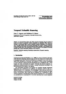
cause they consider time points as the variables of a problem. A time point may be a beginning or an ending point of some event, as well as a neutral point of time. An effective representation of quantitative temporal networks is based on constraints [11]. Definition 1 (TCSP) A Temporal Constraint Satisfaction Problem (TCSP) consists of a set of variables {X1 , . . . , Xn } and a set of unary and binary constraints over pairs of such variables. The variables have continuous or discrete domains; each variable represents a time point. Each constraint is represented by a set of intervals 1 {I1 , . . . , Ik } = {[a1 , b1 ], . . . , [ak , bk ]}. A unary constraint Ti restricts the domain of variable Xi to the given set of intervals; that is, it represents the disjunction (a1 ≤ Xi ≤ b1 ) ∨ . . . ∨ (ak ≤ Xi ≤ bk ). A binary constraint Tij over variables Xi and Xj constrains the permissible values for the distance Xj − Xi ; it represents the disjunction (a1 ≤ Xj − Xi ≤ b1 ) ∨ . . . ∨ (ak ≤ Xj − Xi ≤ bk ). Constraints are assumed to be given in the canonical form in which all intervals are pair-wise disjoint. A TCSP can be represented by a directed constraint graph where nodes represent variables and an edge Xi −→ Xj indicates constraint Tij and it is labeled by the corresponding interval set. A special time point X0 is introduced to represent the “beginning of the world”. All times are relative to X0 ; thus, we can treat each unary constraint Ti as a binary constraint T0i . Example 1 Alice has lunch between noon and 1pm and she wants to go swimming for two hours. She can either go to the pool from 3 to 4 hours before lunch, since she must shower and drive home, or 3 to 4 hours after lunch since it is not safe to swim too soon after a meal. This scenario can be modeled as a TCSP, as shown in Figure 1. There are five variables: X0 , Ls (starting time for lunch), Le (end time for lunch), SS (start swimming), Se (end swimming). For example, the constraint from X0 to Ls states that lunch must be between 12 and 1pm while, the constraint from Ls to Ss states that the distance between the start of the swimming activity and the start of lunch must be either between 3 and 4 hours, or between -4 and -3 hours. Similarly for the other constraints.
[1,1]
Ls [12,13]
X0
Le [−4,−3] [3,4]
Ss
[2,2]
Se
Fig. 1. A TCSP.
Given a TCSP, a tuple of values for its variables, say {v1 , . . . , vn }, is called a solution if the assignment {X1 = v1 , . . . , Xn = vn } does not violate any constraint. A TCSP is said to be consistent if it has a solution. Also, vi is a feasible value for variable Xi if there exists a solution in which Xi = vi . The set of all feasible values for a variable is called its minimal domain. A minimal constraint Tij between Xi and Xj is the set of values v such that v = vj − vi , where vj is a feasible value for Xj and vi is a feasible value for Xi . A TCSP is minimal if its domains and constraints are minimal. It is decomposable if every assignment of values to a set of its variables which does not violate the constraints among such variables can be extended to a solution. Constraint propagation over TCSPs is defined using three binary operations on constraints: union, intersection and composition. Definition 2 Let T = {I1 , . . . , Il } and S = {J1 , . . . ,Jm } be two temporal constraints defined on the pair of variables Xi and Xj . Then: – The Union of T and S, denoted T ∪ S, is: T ∪ S = {I1 , . . . , Il , J1 , . . . , Jm }. – The Intersection of T and S, denoted T ⊕ S, is: T ⊕ S = {Kk = Ii ∩ Jj |i ∈ {1, . . . , l}, j ∈ {1, . . . , }}. Definition 3 Let T = {I1 , . . . , Il } be a temporal constraint defined on variables Xi and Xk and S = {J1 , . . . , Jm } a temporal constraint defined on variables Xk and Xj . Then the composition of T and S, denoted by T ⊗S is a temporal constraint defined on Xi and Xj as follows: T ⊗ S = {K1 , . . . , Kn }, Kh = [a + c, b + d], ∃Ii = [a, b], Jj = [c, d]. Notice that the composition of two temporal constraints, say S and T , defined respectively on 1 For simplicity, we assume closed intervals; however the same applies to semi-open intervals.
5
the pairs of variables (Xi , Xk ) and (Xk , Xj ), is a constraint defined on the pair (Xi , Xj ) which allows only pairs of values, say (vi , vj ), for which there exists a value vk , such that (vi , vk ) satisfies S and (vk , vj ) satisfies T . Given a TCSP, the first interesting problem is to determine its consistency. If the TCSP is consistent, we may wish to find some solutions, or to answer queries concerning the set of all solutions. All these problems are NP-hard [11]. Notions of local consistency may be interesting as well. For example, a TCSP is said to be path consistent iff, for each of its constraint, say Tij , we have Tij ⊆ ⊕∀k (Tik ⊗ Tkj ). A TCSP in which all constraints specify a single interval is called a Simple Temporal Problem. In such a problem, a constraint between Xi and Xj is represented in the constraint graph as an edge Xi −→ Xj labeled by a single interval [aij , bij ] that represents the constraint aij ≤ Xj − Xi ≤ bij . An STP can also be associated with another directed weighted graph Gd = (V, Ed ), called the distance graph, which has the same set of nodes as the constraint graph but twice the number of edges: for each binary constraint over variables Xi and Xj , the distance graph has an edge Xi −→ Xj which is labeled by weight bij , representing the linear inequality Xj − Xi ≤ bij , as well as an edge Xj −→ Xi which is labeled by weight −aij , representing the linear inequality Xi − Xj ≤ −aij . Each path from Xi to Xj in the distance graph Gd , say through variables Xi0 = Xi , Xi1 , Xi2 , . . . , Xik = Xj induces the following path constraint: Pk Xj − Xi ≤ h=1 bih−1 ih . The intersection of all induced path constraints yields the inequality Xj − Xi ≤ dij , where dij is the length of the shortest path from Xi to Xj , if such a length is defined, i.e., if there are no negative cycles in the distance graph. An STP is consistent if and only if its distance graph has no negative cycles [45,20]. This means that enforcing path consistency is sufficient for solving STPs [11]. It follows that a given STP can be effectively specified by another complete directed graph, called a d-graph, where each edge Xi −→ Xj is labeled by the shortest path length dij in the distance graph Gd . In [11] it is shown that any consistent STP is backtrack-free (that is, decomposable) relative to the constraints in its d-graph. Moreover, the set of temporal constraints of the form [−dji , dij ] is the minimal STP corresponding to the original
STP and it is possible to find one of its solutions using a backtrack-free search that simply assigns to each variable any value that satisfies the minimal network constraints compatibly with previous assignments. Two specific solutions (usually called the latest and the earliest one) are given by SL = {d01 , . . . , d0n } and SE = {d10 , . . . , dn0 }, which assign to each variable respectively its latest and earliest possible time [11]. The d-graph (and thus the minimal network) of an STP can be found by applying Floyd-Warshall’s All-P airs-Shortest-P ath algorithm [13] to the distance graph with a complexity of O(n3 ) where n is the number of variables. Since, given the dgraph, a solution can be found in linear time, the overall complexity of solving an STP is polynomial. 2.2. Soft constraints In the literature there are many formalizations of the concept of soft constraints [43,40,32]. Here we refer to the one described in [6,5], which however can be shown to generalize and express many of the others [6,4]. In a few words, a soft constraint is just a classical constraint where each instantiation of its variables has an associated element (also called a preference) from a partially ordered set. Combining constraints will then have to take into account such additional elements, and thus the formalism has also to provide suitable operations for combination (×) and comparison (+) of tuples of preferences and constraints. This is why this formalization is based on the concept of semiring, which is just a set plus two operations. Definition 4 (semirings and c-semirings) A semiring is a tuple hA, +, ×, 0, 1i such that: – A is a set and 0, 1 ∈ A; – + is commutative, associative and 0 is its unit element; – × is associative, distributes over +, 1 is its unit element and 0 is its absorbing element. A c-semiring is a semiring hA, +, ×, 0, 1i such that: – + is defined over possibly infinite sets of elements of A in the following way: P ∗ ∀a ∈ A, ({a}) = a;
6
P P ∗ P(∅) 1; S = 0 and (A) P= P ∗ ( Ai , i ∈ S) = ({ (Ai ), i ∈ S}) for all sets of indexes S, that is, for al sets of subsets of A (flattening property); – × is commutative. Let us consider the relation ≤S over A such that a ≤S b iff a + b = b. Then it is possible to prove that (see [5]): – – – –
≤S is a partial order; + and × are monotone on ≤S ; 0 is its minimum and 1 its maximum; hA, ≤S i is a complete lattice and, for all a, b ∈ A, a + b = lub(a, b).
Moreover, if × is idempotent, then hA, ≤S i is a complete distributive lattice and × is its glb. Informally, the relation ≤S gives us a way to compare (some of the) tuples of preferences and constraints. In fact, when we have a ≤S b, we will say that b is better than (or preferred to) a. Definition 5 (constraints) Given a c-semiring S = hA, +, ×, 0, 1i, a finite set D (the domain of the variables), and an ordered set of variables V , a constraint is a pair hdef, coni where con ⊆ V and def : D|con| → A. Therefore, a constraint specifies a set of variables (the ones in con), and assigns to each tuple of values in D of these variables an element of the semiring set A. This element can be interpreted in many ways: as a level of preference, or as a cost, or as a probability, etc. The correct way to interpret such elements determines the choice of the semiring operations. Definition 6 (SCSP) A soft constraint satisfaction problem is a pair hC, coni where con ⊆ V and C is a set of constraints over V . Note that classical CSPs are isomorphic to SCSPs where the chosen c-semiring is: SCSP = h{f alse, true}, ∨, ∧, f alse, truei. Fuzzy CSPs [40,42] extend the notion of classical CSPs by allowing non crisp constraints, that is, constraints which associate a preference level with each tuple of values. Such level is always between 0 and 1, where 1 represents the best value and 0 the worst one. The solution of a fuzzy CSP is then defined as the set of tuples of values (for all the variables) which have the maximal value.
The way they associate a preference value with an n-tuple is by minimizing the preferences of all its subtuples. The motivation for such a maxmin framework relies on the attempt to maximize the value of the least preferred tuple. It is easy to see that Fuzzy CSPs can be modeled in the SCSP framework by choosing the c-semiring: SF CSP = h[0, 1], max, min, 0, 1i. Definition 7 (combination) Given two constraints c1 = hdef1 , con1 i and c2 = hdef2 , con2 i, their combination c1 ⊗ c2 is the constraint hdef, coni, where con = con1 ∪con2 and def (t) = def1 (t ↓con con1 2 ) ×def2 (t ↓con con2 ) . The combination operator ⊗ can be straightforwardly extended also to finite sets of constraints: when applied N to a finite set of constraints C, we will write C. In words, combining constraints means building a new constraint involving all the variables of the original ones, and which associates to each tuple of domain values for such variables a semiring element which is obtained by multiplying the elements associated by the original constraints with the appropriate subtuples. Definition 8 (projection) Given a constraint c = hdef, coni and a subset I of V , the projection of c over I, written c ⇓I , is the constraint hdef ′ , con′ i where con′ = con ∩ I and def ′ (t′ ) = P t/t↓con =t′ def (t). I∩con
Informally, projecting means eliminating some variables. This is done by associating to each tuple over the remaining variables a semiring element which is the sum of the elements associated by the original constraint with all the extensions of this tuple over the eliminated variables. Definition 9 (solution constraint) The solution constraint of an SCSP problem P = hC, coni is the N constraint Sol(P ) = ( C) ⇓con . That is, to obtain the solution constraint of an SCSP, we combine all constraints, and then project over the variables in con. In this way we get the constraint over con which is “induced” by the entire SCSP. 2 By t ↓X we mean the projection of tuple t, which is Y defined over the set of variables X, over the set of variables Y ⊆ X.
7
Definition 10 (solution) Given an SCSP problem P , consider Sol(P ) = hdef, coni. A solution of P is a pair ht, vi where t is an assignment to all the variables in con and def (t) = v. Definition 11 (optimal solution) Given an SCSP problem P , consider Sol(P ) = hdef, coni. An optimal solution of P is a pair ht, vi such that t is an assignment to all the variables in con, def (t) = v, and there is no t′ , assignment to con, such that v S1
Fig. 2. A Fuzzy CSP and two of its solutions.
SCSPs can be solved by extending and adapting the techniques usually used for classical CSPs. For example, to find the best solution, we could employ a branch-and-bound search algorithm (instead of the classical backtracking). Also the socalled constraint propagation techniques, like arcconsistency [21] and path-consistency, can be generalized to SCSPs [5,6]. The detailed formal definition of constraint propagation (sometimes called also local consistency) for SCSPs can be found in [5,6]. For the purpose of this paper, what is important to say is that a propagation rule is a function which, given an SCSP, generates the solution constraint of a
subproblem of it. It is possible to show that propagation rules are idempotent, monotone, and intensive functions (over the partial order of problems) which do not change the solution constraint. Given a set of propagation rules, a constraint propagation algorithm applies them in any order until stability. It is possible to prove that constraint propagation algorithms defined in this way have the following properties if the multiplicative operation of the semiring is idempotent: equivalence, termination, and uniqueness of the result. Thus we can notice that the generalization of local consistency from classical CSPs to SCSPs concerns the fact that, instead of deleting values or tuples of values, obtaining local consistency in SCSPs means changing the semiring value associated with some tuples or domain elements. The change always brings these values towards the worst value of the semiring, that is, the 0. 2.3. Inductive learning The problem of learning temporal preferences from examples of solutions ratings can be formally described as an inductive learning problem [39,23]. Inductive learning can be defined as the ability of a system to induce the correct structure of a map t(·) which is known only for particular inputs. More formally, defining an example as a pair (x, t(x)), the computational task is as follows: given a collection of examples of t(·), i.e., the training set, return a function h(·) that approximates t(·). Function h(·) is called a hypothesis. A common approach to inductive learning is to evaluate the quality of a hypothesis h on the training set through an error function [15]. An example of a popular error function, that can be used over the reals, Pn is the sum of squares error [15]: SSE = 21 i=1 (t(xi ) − h(xi ))2 , where (xi , t(xi )) is the i-th example of the training set. Other error functions that can be used to evaluate the quality of a hypothesis are the maximum absolute error and mean absolute error, respectively defined as: Emax = max1,...n |t(xi ) − h(xi )|, and P Emed = ( i=1...n |t(xi ) − h(x1 )|)/n. Given a starting hypothesis h0 , the goal of learning is to minimize the chosen error function by modifying h0 . This can be done by using a definition of h which depends on a set of internal parameters W , i.e., h ≡ hW , and then adjusting these parameters. This adjustment can be formulated in different
8
ways, depending on whether their domain is isomorphic to the reals or not. The usual way to be used over the reals, and if hW is continuous and differentiable, is to follow the negative of the gradient of the error function with respect to W . This technique is called gradient descent [15]. Specifically, the set of parameters W is initialized to small random values at time τ = 0 and updated at time τ + 1 according to the following equation, known as ∆-rule: W (τ + 1) = W (τ ) + ∆W (τ ), where ∂E and η is the step size used for the ∆W (τ ) = −η ∂W (τ ) gradient descent, called the learning rate. Learning is usually stopped when a minimum of the error function is reached. Note that, in general, there is no guarantee that the minimum found this way is a global minimum for the function to be learned. Once the learning phase is finished, the resulting function h is evaluated over a set of examples, called the test set, which is disjoint from the training set. The evaluation is done by computing the error, with the same options as for the error computation on the training set. As far as how the examples are used, learning techniques can be divided in two categories: stochastic (also called online) and batch (also called offline) learning. Batch supervised learning is the classical approach in machine learning: a set of examples is obtained and used in order to learn a good approximating function (i.e. train the system), before the system is used. On the other hand, in online learning, data gathered during the normal operation of the system are used to continuously adapt the learned function. For example, in batch learning, when minimizing the sum of squares P error, the sum would be computed as in SSE = 12 ni=1 (t(xi ) − h(xi ))2 , where x1 , . . . , xn are all the examples of the training set. On the other hand, in stochastic learning, the weights are updated after the presentation of each training example, which may be sampled with or without repetition. This corresponds to the minimization of the instantaneous error which, in the case of sum of squares error, would be SSE = 12 (t(xi )−h(xi ))2 when computed on the i-th example. It can be shown that, for sufficiently small values of the learning rate η, stochastic gradient descent converges to the minimum of a batch error function [15]. Although batch learning seems faster for small training sets and systems, stochastic learning is faster for large training sets, it helps escaping local
minima and provides a more natural approach for learning nonstationary tasks [23,2,41,47]. Moreover, stochastic methods seem more robust to errors, omissions or redundant data in the training set can be corrected or ejected during the training phase. Additionally, training data can often be generated easily and in great quantities when the system is in operation, whereas it is usually scarce and precious before. In a broad sense, stochastic learning is essential if the goal is to obtain a learning system as opposed to a merely learned one, as pointed out in [48]. The learning module we will present in Section 6 performs a stochastic gradient descent on SSE.
3. Temporal CSPs with Preferences Although very expressive, TCSPs are able to model just hard temporal constraints. This means that all constraints have to be satisfied, and that the solutions of a constraint are all equally satisfying. However, in many real-life scenarios these two assumptions do not hold. In particular, sometimes some solutions are preferred with respect to others. Therefore the global problem is not to find a way to satisfy all constraints, but to find a way to satisfy them optimally, according to the preferences specified. To address such problems we propose a framework, where each temporal constraint is associated with a preference function, which specifies the preference for each distance or duration. This framework is based on both TCSPs and semiringbased soft constraints. The result is a class of problems which we will call Temporal Constraint Satisfaction Problems with Preferences (TCSPPs). Definition 12 (soft temporal constraint) A soft temporal constraint is a 4-tuple h(X, Y ), I, A, f i consisting of – an ordered pair of variables (X, Y ) over the integers, called the scope of the constraint; – a set of disjoint intervals I = {[a1 , b1 ], . . . , [an , bn ]}, where all ai ’s and bi ’s are integers, and ai ≤ bi for all i = 1, . . . , n; – a set of preferences A; – a preference function f , where Sn f : i=1 [ai , bi ] → A, which is a mapping of the elements belonging to an interval of I into preference values, taken from set A.
9
Given an assignment of the variables X and Y , say vx and vy , we say that this assignment satisfies the constraint h(X, Y ), I, A, f i iff there is [ai , bi ] ∈ I such that ai ≤ vy − vx ≤ bi . In such a case, the preference associated with the assignment by the constraint is f (vy − vx ). Definition 13 (TCSPP) Given a semiring S = hA, +, ×, 0, 1i, a Temporal Constraint Satisfaction Problems with Preferences over S is a pair hV, Ci, where V is a set of variables and C is a set of soft temporal constraints over pairs of variables in V and with preferences in A. Definition 14 (solution) Given a TCSPP hV, Ci over a semiring S, a solution is an assignment to all the variables in V , say t, that satisfies all the constraints in C. An assignment t is said to satisfy a constraint c in C with preference p if the projection of t over the pair of variables of c satisfies c with an associated preference equal to p. We will write pref (t, c) = p. Each solution has a global preference value, obtained by combining, via the × operator of the semiring, the preference levels at which the solution satisfies the constraints in C. Definition 15 (solution’s preference) Given a TCSPP hV, Ci over a semiring S and one of its solutions t = hv1 , . . . , vn i, its preference, denoted by val(t), is computed by Πc∈C pref (s, c), where the product here is performed by using the multiplicative operation of semiring S. The optimal solutions of a TCSPP are those solutions which are not dominated by any other solution in preference terms. Definition 16 (optimal solutions) Given a TCSPP P = hV, Ci over the semiring S, a solution t of P is optimal if for every other solution t′ of P , t′ 6≥S t. To see an instance of TCSPPs, consider TCSPPs over the semiring Sf uzzy = h[0, 1], max, min, 0, 1i, used for fuzzy constraint solving [42]. In this case, the global preference value of a solution is the minimum of all the preference values associated with the distances selected by this solution in all constraints, and the optimal solutions are those with the maximal value. We will use this class of TC-
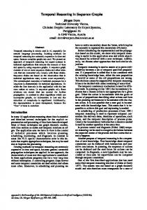
SPPs, also called fuzzy TCSPPs, extensively in this paper. A justification of the the max-min framework adopted in fuzzy TCSPPs is to formalize the criterion of maximizing the value of the least preferred tuple. This can be interpreted as a having a conservative attitude which identifies a solution with its weakest part. Of course other approaches to preferences can be adopted. For example, the weighted semiring can be used, in which preferences are costs, ranging in [0, +∞], and the goal is to minimize the sum of such costs. Such temporal preferences have been considered in [29]. Example 3 Consider again the scenario described in Example 1, where Alice can go swimming either before or after lunch. Alice might, for example, prefer to have lunch as early as possible. Moreover, if she goes swimming in the morning, she might want to go as late as possible so she can sleep longer, while, if she goes in the afternoon, she might prefer to go as early as possible so she will have more time to get ready for the evening. These preferences can be represented using a weighted TCSPP or a fuzzy TCSPP as shown, respectively, in Figure 3 part (a) and (b). It is easy to see that the assignment hLs = 12, Ss = 15i (we omitted X0 since we assume its value always to be 0) is an optimal solution, since it has the minimum cost, that is, 0, in the weighted TCSPP and maximum preference, that is, 1, in the fuzzy TCSPP. Notice that our framework is a generalization of TCSPs, since TCSPs are just TCSPPs over the the semiring Scsp = h{f alse, true}, ∨, ∧, f alse, truei, which allows to describe hard constraint problems [22]. As for TCSPs, a special instance of TCSPPs is characterized by a single interval in each constraint. We call such problems Simple Temporal Problems with Preferences (STPPs), since they generalize Simple Temporal Problems (STPs) [11]. This case is interesting because, as noted above, STPs are polynomially solvable, while general TCSPs are NP-hard, and the computational effect of adding preferences to STPs is not immediately obvious. STPPs are also expressive enough to represent many real life scenarios. Example 4 Consider the Landsat 7 example given in the introduction. In Figure 4 we show an STPP
10 f(L S−X0 )
3.1. Complexity of solving TCSPPs and STPPs
f(S S−L ) S
10
10
Ls 0 12
0 −4
13 L −X S 0
X0
3
−3
4 S −L S S
Ss
(a)
f(L S−X0 )
f(S S−L ) S
1 1
0.7
12
Ls
0.5
13 L −X S 0
−4
X0
−3
3
4
S S−LS
Theorem 1 (Complexity of STPPs) Solving STPPs is NP-hard.
Ss
(b)
Fig. 3. The constraint graphs of a Weighted TCSPP (a) and of a Fuzzy TCSPP (b).
that models it. There are 3 events to be scheduled: the start time (Ss ) and ending time (Se ) of a slewing activity, and the start time of an image retrieval activity (Is ). Here the beginning of time is represented by variable Ss . The slewing activity in this example can take from 3 to 10 units of time, but it is preferred that it takes the shortest time possible. This is modeled by the constraint from Ss to Se . The image taking can start any time between 3 and 20 units of time after the slewing has been initiated. This is described by the constraint from Ss to Is . The third constraint, from Se to Is , models the fact that it is better for the image taking to start as soon as the slewing has stopped. f(Se−Ss) 11 1 0.9
0.8 0.7 0.6 0.5
3 4 5 6 7
8 9 10
Ss
Se−Ss Se
f(Is−Ss)
f(Is−Se)
1
1 1 1 0.9
0.9 0.8
0.8
0.7
0.7
0.6
0.6 3
20
Is−Ss Is
As noted in Section 2, TCSPs are NP-hard problems. Since the addition of preference functions can only make the problem of finding the optimal solutions more complex, it is obvious that TCSPPs are NP-hard problems as well. In fact, TCSPs are just TCSPPs over the SCSP semiring. We now turn our attention to the complexity of general STPPs. We recall that STPs are polynomially solvable, thus one might speculate that the same is true for STPPs. However, it is possible to show that, in general, STPPs fall into the class of NP-hard problems.
−4 −3 −2 −1
0 1 2 3
4
5
6
Fig. 4. The STPP for the Landsat 7 example.
Is−Se
Proof: We prove this result by reducing an arbitrary TCSP to an STPP. Consider a TCSP, and take any of its constraints, say I = {[a1 , b1 ], . . . [an , bn ]}. We will now obtain a corresponding soft temporal constraint containing just one interval (thus belonging to an STPP). The semiring that we will use for the resulting STPP is the classical one: Scsp = h{f alse, true}, ∨, ∧, f alse, truei. Thus the only allowed preference values are f alse and true. Assuming that the intervals in I are ordered such that ai ≤ ai+1 for i ∈ {1, . . . , n − 1}, the interval of the soft constraint is just [a1 , bn ]. The preference function will give value true to all elements belonging to an interval in I and f alse to the others. Thus we have obtained an STPP whose set of solutions with value 1 (which are the optimal solutions, since f alse ≤S true in the chosen semiring) coincides with the set of solutions of the given TCSP. Since finding the set of solutions of a TCSP is NP-hard, it follows that the problem of finding the set of optimal solutions to an STPP is NPhard. 2 However, in the following of the paper we will show there are classes of STPPs which are polynomially solvable: a sufficient condition is having semi-convex preference functions and a semiring with a total order of preference values and an idempotent multiplicative operation. In [12] it has been shown that the only aggregation operator on a totally ordered set that is idempotent is min, i.e. the multiplicative operator of the SF CSP semiring.
11
3.2. Path consistency for TCSPPs Given a constraint network, it is often useful to find the corresponding minimal network in which the constraints are as explicit as possible. This task is normally performed by enforcing various levels of local consistency. For TCSPPs, in particular, we can define a notion of path consistency by just extending the notion of path consistency for TCSPs [11]. Given two soft constraints, and a semiring S, we define: – the intersection of two soft constraints Tij and Tij′ , defined on the same pair of variables, written Tij ⊕S Tij′ , as the soft temporal con′ straint Tij′′ = hIij ⊕ Iij , f i, where: ′ ∗ Iij ⊕ Iij is the pairwise intersection of in′ tervals in Iij and Iij , and ′ ∗ f (a) = fij (a) ×S fij′ (a) for all a ∈ Iij ⊕ Iij .
– the composition of two soft constraints Tik and Tkj , with variable Xk in common, written Tik ⊗S Tkj , as the soft constraint Tij = hIik ⊗ Ikj , f i, defined on variables Xi and Xj , where: ∗ a ∈ Iik ⊗ Ikj iff there exists a value a1 ∈ Iik and a2 ∈ P Ikj such that a = a1 + a2 , and ∗ f (a) = {fik (a1 ) ×S fkj (a2 )|a = a1 + a2 , a1 ∈ Iik , a2 ∈ Ikj }. The path-induced constraint on variables Xi and path Xj is Rij = ⊕S ∀k(Tik ⊗S Tkj ), i.e., the result of performing ⊕S on each way of generating paths of length two from Xi to Xj . A constraint Tij is path , i.e., Tij is at least path-consistent iff Tij ⊆ Rij path . A TCSPP is path-consistent iff as strict as Rij all its constraints are path-consistent. It is interesting to study under which assumptions, by applying the path consistency operation Tij := Tij ⊕S (Tik ⊗S Tkj ) to any constraint of a given TCSPP, the resulting TCSPP is equivalent to the given one, that is, it has the same set of solutions with the same preferences. The assumptions can be derived directly from those which are sufficient in generic SCSPs, as stated by the following theorem. Theorem 2 Consider an TCSPP P defined on a semiring which has an idempotent multiplicative operator. Then, applying operation Tij := Tij ⊕S (Tik ⊗S Tkj ) for any k to any constraint Tij of P returns an equivalent TCSPP.
Proof: Consider TCSPPs P1 and P2 on the same set of variables {X1 , . . . , Xn } and defined over a semiring with an idempotent multiplicative operator. Assume also that the set of constraints of P2 consists of the constraints of P1 minus {Tij } plus {Tij ⊕S (Tik ⊗S Tkj )}. To show that P1 is equivalent to P2 we must show that every solution t of P1 with preference val(t) is a solution of P2 with the same preference. Notice that P1 and P2 differ only for the constraint defined on variables Xi and Xj , which is Tij = hI, f i in P1 and Tij′ = Tij ⊕S (Tik ⊗S Tkj ) = hI ′ , f ′ i in P2 , where Tik = hIik , fik i and Tkj = hIkj , fkj i are the same in P1 and P2 . Now, since Tij′ = Tij ⊕S (Tik ⊗S Tkj ) = hI ′ , f ′ i, then I ′ = I ⊕ (I1 ⊗ I2 ). This means that I ′ ⊆ I. Assuming I ′ ⊂ I, we will now show that no element a ∈ I-I ′ can be a projection of a solution s of P1 . Assume to the contrary that s is a solution of P1 such that s ↓Xi ,Xj = (si , sj ) and sj − si = a ∈ I-I ′ . Then, since a 6∈ I ′ means that there is no a1 ∈ Iik nor a2 ∈ Ikj such that a = a1 + a2 , then either sk − si = a1 6∈ Iik or sj − sk = a2 6∈ Ikj . But this cannot be the case, since s is assumed to be a solution of P1 . From the above argument we can conclude that, for any solution t of P1 , we have t ↓Xi ,Xj ∈ I ′ . Thus P1 and P2 have the same set of solutions. Consider solution t in P1 . Then, as stated in the previous section, the global preference associated with t in P1 is val(t) = ×{fpq (vq − vp )|(vp , vq ) = t ↓Xp ,Xq }, which can be rewritten, highlighting the preferences obtained on constraints Tij , Tik and Tkj , as: val(t) = f (vj −vi )×f (vk −vi )×f (vj −vk )× B, where B = ×{fpq (vq − vp )|(vp , vq ) = t ↓Xp ,Xq , (p, q) 6∈ {(i, j), (k, i), (j, k)}}. Similarly, in P2 the global preference of t is val′ (t) = f ′ (vj −vi )×f (vk −vi )×f (vj −vk )×B. We want to prove that val(t) = val′ (t). Notice that B appears in val(t) and in val′ (t), hence we can ignore it. ByP definition: f ′ (vj − vi ) = f (vj − vi ) × Q where Q = v′ |(v′ −vi )∈Iik ,(vj −v′ )∈Ikj [f (vk′ − vi ) × f (vj − k k k vk′ )]. Now, among the possible assignments to variable Xk , say vk′ , such that (vk′ − vi ) ∈ Iik and (vj − vk′ ) ∈ Ikj , there is the assignment given to Xk in solution t, say vk . Thus we rewrite f ′ (vj − vi ) in the following way: f ′ (vj − vi ) = f (vj − vi ) × {[f (vk − vi ) × f (vj − vk )] +
12
P
[f (vk′ −vi )×f (vj − ′ |(v ′ −v )∈I ,(v −v ′ )∈I ′ vk i j ik kj ,vk 6=vk k k
vk′ )]}.
At this point, the preference of solution t in P2
is ′ f (vj − vk )] + Pval (t) = f (vj − vi ) × {[f (vk − vi ) × ′ [f (v −v ′ ′ ′ ′ i )×f (vj − k vk |(vk −vi )∈Iik ,(vj −vk )∈Ikj ,vk 6=vk vk′ )]} × f (vk − vi ) × f (vj − vk ) × B. We will now show a property that holds for any two elements a, b ∈ A of a semiring with an idempotent multiplicative operator: a × (a + b) = a. In [6] it is shown that × is intensive with respect to the ordering of the semiring, that is, for any a, c ∈ A we have a × c ≤S a. In particular this holds for c = (a + b) and thus a × (a + b) ≤S a. On the other hand, since a + b is the lub of a and b, (a+b) ≥S a, and by monotonicity of × we get that a×(a+b) ≥ a×a. At this point we use the idempotency assumption on × and obtain a × a = a and, thus, a × (a + b) ≥S a. Therefore a × (a + b) = a. We now use this result in the formula describing val′ (t), P setting a = (f (vk − vi ) × f (vj − vk )), and b = v′ |(v′ −vi )∈Iik ,(vj −v′ )∈Ikj ,v′ 6=vk [f (vk′ − vi ) × k k k k f (vj −vk′ )]. We obtain: val′ (t) = f (vj −vi )×f (vk − vi ) × f (vj − vk ) × B, which is exactly val(t). 2 Under the same condition, applying this operation to a set of constraints (rather than just one) returns a final TCSPP which is always the same independently of the order of application. Again, this result can be derived from the more general results that hold for SCSPs [6], as shown by following theorem.
Theorem 3 Consider an TCSPP P defined on a semiring with an idempotent multiplicative operator. Then, applying operation Tij := Tij ⊕S (Tik ⊗S Tkj ) to a set of constraints of P returns the same final TCSPP regardless of the order of application. Proof: Applying operation Tij := Tij ⊕S (Tik ⊗S Tkj ) can be seen as applying a function f to an TCSPP P that returns another TCSPP f (P ) = P ′ . The local consistency algorithm that applies this operation until quiescence can thus be seen as the repetitive application of function f . As in the case of generic SCSPs, it is possible to use a result of classical chaotic theory [9] that ensures the independence of the result on the order of application of closure operators, that is, functions that are idempotent, monotone and intensive. We will now prove that function f satisfies such requirements if the multiplicative operator is idempotent. In par-
ticular, under such an assumption, function f is: Idempotent: In fact, applying twice operation Tij := Tij ⊕S (Tik ⊗S Tkj ) to constraint Tij , when constraints Tik and Tkj have not changed, gives the same result as applying it only once; Monotone: Consider the ordering on SCSPs defined in [6]. Such ordering can be redefined here as follows: given TCSPP P1 and TCSPP P2 we 1 say that P1 ≤P P2 iff for every constraint Tpq = 1 1 2 hIpq , fpq i in P1 and corresponding constraint Tpq = 2 2 1 2 1 hIpq , fpq i in P2 , then Ipq ⊆ Ipq and ∀w ∈ Ipq we 1 2 have fpq (w) ≤ fpq (w). If now we apply operation f to P1 and P2 we get two new TCSPPs, f (P1 ) and f (P2 ), that differ respectively from P1 and P2 only on constraint Tij1 and Tij2 . By intensivity of ×, applying Tij := Tij ⊕S (Tik ⊗S Tkj ) to a constraint can only shrink its interval and lower the preferences corresponding to the remaining elements. Since this change depends only on the preferences on constraints Tik and Tkj , and by assumption we 1 2 1 2 have that Tik ≤P Tik and Tkj ≤P Tkj , by monotonicity of × the new preferences in constraint Tij1 in f (P1 ) are smaller than or equal to those on constraint Tij2 in problem f (P2 ). Intensive: That is, f (P1 ) ≤P P1 for any TCSPP P1 . In fact, as mentioned in the previous point, f (P1 ) differs from P1 only by constraint Tij . However, f ensures that constraint Tij in f (P1 ) can only have a smaller or equal interval with respect to that in P1 and that remaining elements can have preferences smaller than or equal to the ones in P1 . 2 Thus any TCSPP can be transformed into an equivalent path-consistent TCSPP by applying the operation Tij := Tij ⊕S (Tik ⊗S Tkj ) to all constraints Tij until no change occurs on any constraint. We will call this path consistency enforcing algorithm TCSPP PC-2 when applied to an TCSPP and STPP PC-2 when applied to an STPP. Figure 5 shows the TCSPP obtained by applying path consistency to the TCSPP in Figure 3. Path consistency is proven to be polynomial for TCSPs, with complexity O(n3 R3 ), where n is the number of variables and R is the range of the constraints [11]. However, applying it is, in general, not sufficient to find a solution. Again, since a TCSP is a special instance of TCSPP over the SCSP semiring, applying path consistency is not sufficient to find an optimal solution of an TCSPP either. On the other hand, with STPPs over the same semiring, that is STPs, applying STPP PC-2
13 f(LS −X) 0 1
Ls
0.7
12
f(SS−L) S
−3
3
0.5
−4
X0
4
S S−LS
Ss
1
1 0.7
0.7
0.5
0.2
8
1
0.2
13 L −X S 0
f(SS−X) 0
1
9
10
15
16
17
S S−X0
Fig. 5. The path consistent constraint graph of the TCSPP in Figure 3.
is sufficient [11]. It is easy to infer that the hardness result for STPPs, given in Section 3.1, derives either from the nature of the semiring or from the shape of the preference functions. 3.3. Semi-convexity and path consistency When the preference functions are linear, and the semiring chosen is such that its two operations maintain such linearity when applied to the initial preference function, it can be seen that the initial STPP can be written as a linear programming problem, solving which is tractable [8]. In fact, consider any given TCSPP. For any pair of variables X and Y , take each interval for the constraint over X and Y , say [a, b], with associated linear preference function f . The information given by each of such intervals can be represented by the following inequalities and equation: X − Y ≤ b, Y − X ≤ −a and fX,Y = c1 (X − Y ) + c2 . Then if we choose the fuzzy semiring SF CSP = h[0, 1], max, min, 0, 1i, the global preference value V will satisfy the inequality V ≤ fX,Y for each preference function fX,Y defined in the problem, and the objective function is max(V ). If instead we choose the semiring hR, min, +, ∞, 0i, where the objective is to minimize the sum of the preference level, we have V = f1 + . . . + fn 3 and the objective function is min(V ) . In both cases, the resulting set of formulas constitutes a linear programming problem. Linear preference functions are expressive enough in many cases, but there are also several situations in which we need preference functions which are not linear. A typical example arises when we want to state that the distance between two events must 3 In this context, the “+” is to be interpreted as arithmetic “+”.
be as close as possible to a single value. Then, unless this value is one of the extremes of the interval, the preference function is convex, but not linear. Another case is one in which preferred values are as close as possible to a single distance value, but in which there are some subintervals where all values have the same preference. In this case, the preference criteria define a step function, which is not even convex. We consider the class of semi-convex functions which includes linear, convex, and also some step functions. More formally, a semi-convex function f is one such that, for all y ∈ ℜ+ , the set {x ∈ X such that f (x) ≥ y} forms an interval. For example, the close to k criteria cannot be coded into a linear preference function, but it can be specified by a semi-convex preference function, which could be f (x) = x for x ≤ k and f (x) = 2k −x for x > k. Figure 6 shows some examples of semi-convex and non-semi-convex functions. (a)
(d)
(g)
(b)
(c)
(e)
(h)
(f)
(i)
Fig. 6. Examples of semi-convex functions [(a)-(f)] and non-semi-convex functions [(g)-(i)]
Semi-convex functions are closed under the operations of intersection and composition, when certain semirings are chosen. For example, this happens with the fuzzy semiring, where the intersection performs the min and composition performs the max operation. Theorem 4 (closure under intersection) Given two semi-convex preference functions f1 and f2 which return values over a totally-ordered semiring S = hA, +, ×, 0, 1i with an idempotent multiplicative operator ×, let f be defined as f (a) = f1 (a)×f2 (a). Then, f is a semi-convex function as well. Proof: Given any y, consider the set {x : f (x) ≥ y}, which by definition coincides with = {x :
14
f1 (x) × f2 (x) ≥ y}. Since × is idempotent then we also have f1 (x) × f2 (x) = glb(f1 (x), f2 (x)). Moreover, since S is totally ordered, we have glb(f1 (x), f2 (x)) = min(f1 (x), f2 (x)), that is the glb coincides with one of the two elements, that is the minimum of the two [6]. Thus, we have {x : f1 (x) × f2 (x) ≥ y} = {x : min(f1 (x), f2 (x)) ≥ y}. Of course, {x : min(f1 (x), f2 (x)) ≥ y} = {x : f1 (x) ≥ y and f2 (x) ≥ y} = {x : x ∈ [a1 , b1 ] and x ∈ [a2 , b2 ]} since each of f1 and f2 is semi-convex. Now, by definition, {x : x ∈ [a1 , b1 ] and x ∈ [a2 , b2 ]} = [a1 , b1 ] ∩ [a2 , b2 ] = [max(a1 , a2 ), min(b1 , b2 )]. We have thus proven the semi-convexity of f , since {x : f (x) ≥ y} is a unique interval. 2 A similar result holds for the composition of semi-convex functions: Theorem 5 (closure under composition) Given a totally ordered semiring with an idempotent multiplicative operation ×, let f1 and f2 be semi-convex functions which return P values over the semiring. Define f as f (a) = b+c=a (f1 (b) × f2 (c)), where b + c is the sum of two integers. Then f is semiconvex. Proof: From the definition of semi-convex functions, it suffices to prove that, for any given y, the set S = {x : f (x) ≥ y} identifies a unique interval. If S is empty, then it identifies the empty interval. In the following we assume S to be not empty. PBy definition of f : {x : f (x) ≥ y} = {x : y}, where u + v is the u+v=x (f1 (u) × f2 (v)) ≥P sum of two integers and generalizes the additive operator of the semiring. In any semiring, the additive operator is the lub operator. Moreover, if the semiring has an idempotent × operator and is totally ordered, the lub of a finite set P is the maximum element of the set. Thus, {x : u+v=x (f1 (u)× f2 (v)) ≥ y} = {x : maxu+v=x (f1 (u) × f2 (v)) ≥ y} which coincides with {x : ∃u, v | x = u + v and (f1 (u) × f2 (v)) ≥ y}.
Using the same steps as in the proof of Theorem 4, we have: {x : ∃u, v | x = u + v and (f1 (u) × f2 (v)) ≥ y} = {x : ∃u, v | x = u + v and min(f1 (u), f2 (v)) ≥ y}. But this set coincides with {x : ∃u, v | x = u + v and f1 (x) ≥ y and f2 (x) ≥ y} = {x : ∃u, v | x = u + v and ∃a1 , b1 , a2 , b2 | u ∈ [a1 , b1 ] and v ∈ [a2 , b2 ]} since each of f1 and f2 is semi-convex. This last set coincides with {x : x ∈ [a1 + a2 , b1 + b2 ]}. We have thus shown the semi-convexity of a function ob-
tained by combining semi-convex preference functions. 2 These results imply that applying the STPP PC2 algorithm to an STPP with only semi-convex preference functions, and whose underlying semiring contains a multiplicative operation that is idempotent and a totally ordered preference set, will result in an STPP whose induced soft constraints have only semi-convex preference functions. Consider now an STPP with semi-convex preference functions and defined on a semiring with an idempotent multiplicative operator and a totally ordered preference set, like SF CSP = h[0, 1] max, min, 0, 1i. In the following theorem we will prove that, if such an STPP is also path consistent, then all its preference functions must have the same maximum preference value. Theorem 6 Consider a path consistent STPP P with semi-convex functions defined on a totallyordered semiring with an idempotent multiplicative operator. Then all its preference functions have the same maximum preference. Proof: All the preference functions of an STPP have the same maximum iff any pair of soft temporal constraints of the STPP is such that their preference function have the same maximum. Notice that the theorem trivially holds if there are only two variables. In fact, in this case, path consistency is reduced to performing the intersection on all the constraints defined on the two variables and a single constraint is obtained. For the following of the proof we will denote with TIJ = hIIJ , fIJ i the soft temporal constraint defined on variables I and J. Let us now assume that there is a pair of constraints, say TAB and TCD , such that ∀h ∈ IAB , fAB (h) ≤ M , and ∃r ∈ IAB , fAB (r) = M , and ∀g ∈ ICD , fCD (g) ≤ m, and ∃s ∈ ICD , fCD (s) = m and M > m. Let us first note that any soft temporal constraint defined on the pair of variables (I, J) induces a constraint on the pair (J, I), such that maxh∈IIJ fIJ (h) = maxg∈IJI fJI (g). In fact, assume that IIJ = [l, u]. This constraint is satisfied by all pairs of assignments to I and J, say vI and vJ , such that l ≤ vJ − vI ≤ u. These inequalities hold iff −u ≤ vI − vJ ≤ −l hold. Thus the interval of constraint TJI must be [−u, −l]. Since each assignment vJ to J and vI to I which identifies
15
element h ∈ [l, u] with a preference fIJ (x) = p identifies element −x ∈ [−u, −l], it must be that fIJ (x) = fJI (−x). Thus fIJ and fJI have the same maximum on the respective intervals. Consider now the triangle of constraints TAC , TAD and TDC . To do this, we assume that, for any three variables, there are constraints connecting every pair of them. This is without loss of generality because we assume to work with a pathconsistent STPP. Given any element a of IAC , since the STPP is P path consistent it must be that: fAC (a) ≤ a1 +a2 =a (fAD (a1 )× fDC (a2 )), where a1 is in IAD and a2 is in IDC . Let us denote with max(fIJ ) the maximum of the preference function of the constraint defined on variables I and J on interval IIJ . Then, since × and + P are monotone, the following must hold: fAC (a) ≤ a1 +a2 =a ((fAD (a1 )×fDC (a2 ))) ≤ max(fAD )×max(fDC ). Notice that this must hold for every element a of IAC , thus also for those with maximum preference, thus: max(fAC ) ≤ max(fAD ) × max(fDC ). Now, since × is intensive, we have max(fAD ) × max(fDC ) ≤ max(fDC ). Therefore, max(fAC ) ≤ max(fDC ) = m. Similarly, if we consider the triangle of constraints TCB , TCD , and TDB we can conclude that max(fCB ) ≤ max(fCD ) = m. We now consider the triangle of constraints TAB , TAC and TCB . Since the STPP is path consistent, then max(fAB ) ≤ max(fAC ) and max(fAB ) ≤ max(fCB ). But this implies that max(fAB ) ≤ m, which contradicts the hypothesis that max(fAB ) = M > m. 2 Consider an STPP P that satisfies the hypothesis of Theorem 6 having, hence, the same maximum preference M on every preference function. Consider the STP P ′ obtained by P taking the subintervals of elements mapped on each constraint into preference M . In the following theorem we will show that, if P is a path consistent STPP, then P ′ is a path consistent STP.
Proof: An STP is path consistent iff all its constraints are path consistent, that is, for every constraint TAB , we have TAB ⊆ ⊕K (TAK ⊗ TKB ), where K varies over the set of variables of the STP [11]. Assume that P ′ is not path consistent. Then there must be at least a hard temporal constraint of P ′ , say TAB , defined on variables A and B, such that there is at least a variable C, with C 6= A and C 6= B, such that TAB 6⊂ TAC ⊗TCB . Let [l1 , u1 ] be the interval of constraint TAB , [l2 , u2 ] the interval of constraint TAC and [l3 , u3 ] the interval of constraint TCB . The interval of constraint TAC ⊗ TCB is, by definition, [l2 + l3 , u2 + u3 ]. Since we are assuming that TAB 6⊂ TAC ⊗ TCB , it must be that l1 < l2 + l3 , or u2 + u3 < u1 , or both. Let us first assume that l1 < l2 + l3 holds. Now, since l1 is an element of an interval of P ′ , by Theorem 6 it must be that fAB (l1 ) = M , where fAB is the preference function of the constraint defined on A and B in STPP P and M is the highest preference in all the constraints of P . Since P is path consistent, then there must be at least a pair of elements, say a1 and a2 , such that a1 ∈ IAC (where IAC is the interval of the constraint defined on A and C in P ), a2 ∈ ICB (where ICB is the interval of the constraint defined on C and B in P ), l1 = a1 + a2 , and fAC (a1 ) × fCB (a2 )) = M . Since × is idempotent and M is the maximum preference on any constraint of P , it must be that fAC (a1 ) = M and fCB (a2 ) = M . Thus, a1 ∈ [l2 , u2 ] and a2 ∈ [l3 , u3 ]. Therefore, it must be that l2 + l3 ≤ a1 + a2 ≤ u2 + u3 . But this is in contradiction with the fact that l1 = a1 + a2 and l1 < l2 + l3 . Similarly for the case in which u2 + u3 < u1 . 2 Notice the the above theorem, and the fact that an STP is path consistent iff it is consistent (i.e., it has at least a solution) [11] allows us to conclude that if an STPP is path consistent, then there is at least a solution with preference M . In the theorem that follows we will claim that M is also the highest preference assigned to any solution of the STPP.
Theorem 7 Consider a path consistent STPP P with semi-convex functions defined on a totally ordered semiring with idempotent multiplicative operator. Consider now the STP P ′ obtained from P by considering on each constraint only the subinterval mapped by the preference function into its maximal value for that interval. Then, P ′ is a path consistent STP.
Theorem 8 Consider a path consistent STPP P with semi-convex functions defined on a totallyordered semiring with idempotent multiplicative operator and with maximum preference M on each function. Consider now the STP P ′ obtained from P by considering on each constraint only the subinterval mapped by the preference function into M . Then, the set of optimal solutions of P is the set of solutions of P ′ .
16
Proof: Let us call Opt(P ) the set of optimal solutions of P , and assume they all have preference opt. Let us also call Sol(P ′ ) the set of solutions of P ′ . By Theorem 7, since P is path consistent and hence globally consistent, we have Sol(P ′ ) 6= ∅. First we show that Opt(P ) ⊆ Sol(P ′ ). Assume that there is an optimal solution s ∈ Opt(P ) which is not a solution of P ′ . Since s is not a solution of P ′ , there must be at least a hard constraint ′ of P ′ , say Iij on variables Xi and Xj , which is violated by s. This means that the values vi and vj which are assigned to variables Xi and Xj by ′ s are such that vj − vi 6∈ Iij . We can deduce from ′ how P is defined, that vj − vi cannot be mapped into the optimal preference in the corresponding soft constraint in P , Tij = hIij , fij i. This implies that the global preference assigned to s, say f (s), is such that f (s) ≤ fij (vj − vi ) < opt. Hence s 6∈ Opt(P ) which contradicts out hypothesis. We now show Sol(P ′ ) ⊆ Opt(P ). Take any solution t of P ′ . Since all the intervals of P ′ are subintervals of those of P , t is a solution of P as well. In fact, t assigns to all variables values that belong to intervals in P ′ and are hence mapped into the optimal preference in P . This allows us to conclude that t ∈ Opt(P ). 2
4. Solving Simple Temporal Problems with Preferences In this section we will describe two solvers for STPPs. Both find an STP such that all its solutions are optimal solutions of the STPP given in input. Both solvers require the tractability assumptions on the shape of the preference functions and on the underlying semiring, to hold. In particular, we will consider semi-convex preferences based on the fuzzy semiring. 4.1. Path-solver: a solver based on path consistency The theoretical results of the previous section can be translated in practice as follows: to find an optimal solution for an STPP, we can first apply path-consistency and then use a search procedure to find a solution without the need to backtrack. Summarizing, we have shown that: (1) Semi-convex functions are closed w.r.t. pathconsistency: if we start from an STPP P with semi-
Pseudocode for path-solver 1. input STPP P; 2. STPP P’=STPP PC-2(P); 3. if P’ inconsistent then return ∅; 4. STP P”=REDUCE TO BEST(P’); 5. return EARLIEST BEST(P”). Fig. 7. Path-solver.
convex functions, and we apply path-consistency, we get a new STPP P ′ with semi-convex functions (by Theorems 4 and 5); the only difference in the two problems is that the new one can have smaller intervals and worse preference values in the preference functions. (2) After applying path-consistency, all preference functions in P ′ have the same best preference level (by Theorem 6). (3) Consider the STP obtained from the STPP P ′ by taking, for each constraint, the sub-interval corresponding to the best preference level; then, the solutions of such an STP coincide with the best solutions of the original P (and also of P ′ ). Therefore, finding a solution of this STP means finding an optimal solution of P . Our first solving module, which we call pathsolver, relies on these results. In fact, the solver takes as input an STPP with semi-convex preference functions, and returns an optimal solution of the given problem, working as follows and as shown in Figure 7: First, in line 2 pathconsistency is applied to the given problem, by function STPP PC-2, producing a new problem P ′ . Then, in line 4 an STP corresponding to P ′ is constructed, applying REDUCE TO BEST to P ′ , by taking the subintervals corresponding to the best preference level and forgetting about the preference functions. Finally, a backtrack-free search is performed to find a solution of the STP, specifically the earliest one is returned by function EARLIEST BEST in line 5. All these steps are polynomial, so the overall complexity of solving an STPP with the above assumptions is polynomial, as stated by the following theorem. Theorem 9 Given an STPP with semi-convex preference functions, defined on a semiring with an idempotent multiplicative operator, with n variables, maximum size of intervals r, and l distinct totally ordered preference levels, the complexity of path-solver is O(n3 rl).
17
Proof: Let us follow the steps performed by pathsolver to solve an STPP. First we apply STPP PC2. This algorithm must consider n2 triangles. For each of them, in the worst case, only one of the preference values assigned to the r different elements is moved down of a single preference level. This means that we can have O(rl) steps for each triangle. After each triangle is visited, at most n new triangles are added to the queue. If we assume that each step which updates Tij needs constant time, we can conclude that the complexity of STPP PC-2 is O(n3 rl). After STPP PC-2 has finished, the optimal solution must be found. Path-solver achieves this by finding a solution of the STPP P ′′ , obtained from P ′ by considering only intervals mapped into maximum preference on each constraint. In [11] it has been shown that this can be done without backtracking in n steps (see also Section 2.1). At each step, a value is assigned to a new variable while not violating the constraints that relate this variable with the previously assigned variables. Assume there are d possible values left in the domain of the variable, then the compatibility of each value must be checked on at most n−1 constraints. Since for each variable the cost of finding a consistent assignment is O(rd), the total cost of finding a complete solution of P ′ is O(n2 d). The complexity of this phase is clearly dominated by that of STPP PC-2. This allows us to conclude that the total complexity of finding an optimal solution of P is O(n3 rl). 2 In the above proof we have assumed that each step of STPP PC-2 Tij := Tij ⊕S (Tik ⊗S Tkj ) is performed in constant time. If we count the arithmetic operations performed during this step, we can see that there are O(r3 ) of them. In fact, each constraint of the triangle has at most r elements in the interval, and, for each element of the interval in constraint Tij , the preference of O(r2 ) decompositions must be checked. With this measure, the new complexity of finding an optimal solution is O(r4 n3 l). Example 5 In Figure 8 we show the effect of applying path-solver on the example in Figure 4. As it can be seen, the interval on the constraint on variables Ss and Is has been reduced from [3,20] to [3,14] and some preferences on all the constraints have been lowered. It is easy to see that the optimal preference of the STPP is 1 and the minimal STP
containing all optimal solutions restricts the duration of the slewing to interval [4,5], the interleaving time between the slewing start and the image start to [3,5] and the interleaving time between the slewing stop and the image start to [0,1]. f(Se−Ss) 1 1 0.9
0.9
0.8 0.7 0.6 0.5
3 4
5 6
7
8
9 10
Se−Ss
Ss
Se
f(Is−Ss) f(Is−Se)
1 0.9
1 1 0.8
0.9
0.9
0.7
0.8
0.8
0.6
0.7
0.7
0.5
0.6
0.6 3
14
0.5
Is−Ss Is
−4 −3 −2 −1
0 1
2
3
4
5
6
Is−Se
Fig. 8. The STPP representing the Landsat 7 scenario depicted in Figure 4 after applying STPP PC-2.
An approach similar to that in path-solver is proposed in [49], in which Fuzzy Temporal Constraint Networks are defined. In such networks, fuzzy intervals are used to model a possibility distribution (see [50]) over intervals. Although our work and the work in [49] have two completely different goals, since ours is to model temporal flexibility in terms of preferences, while in [49] they consider vagueness of temporal relations, there are many points in common. In fact, despite the different semantics, the framework is very close to ours since they give results for Fuzzy Simple Temporal Problems with unimodal possibility distribution, where unimodal is a synonym of semi-convexity. Thus, they combine the possibilities with min and compare them with max, as we do with preferences. To test whether a fuzzy temporal network is consistent, they propose a generalization of the classical path consistency algorithm (PC-1)[24], while we extend the more efficient version for TCSPs (PC-2) proposed in [11]. They compute the minimal network and detect inconsistency if an interval becomes empty. However, they do not prove that after path consistency the possibilities are all lowered to the same maximum and that the STP obtained considering only intervals mapped into that maximum is also minimal. This is what allows us to find an optimal solution in polynomial time. Another difference is that our approach is more general, since TCSPPs can model other classes of preferences than just fuzzy ones.
18
We will show in Section 5.4 that, also because of its generality, the path consistency approach is substantially slower in practice than the chopping solver that we will describe in the next section. 4.2. Chop-solver Given an STPP and an underlying semiring with set of preference values A, let y ∈ A and hI, f i be a soft constraint defined on variables Xi and Xj in the STPP, where f is semi-convex. Consider the interval defined by {x : x ∈ I and f (x) ≥ y}. Since f is semi-convex, this set defines a single interval for any choice of y. Let this interval define a constraint on the same pair Xi and Xj . Performing this transformation on each soft constraint in the original STPP results in an STP, which we refer to as ST Py . Notice that this procedure is related to what are know as α-cuts in fuzzy set theory [19]. Not every choice of y will yield an STP that is solvable. Let opt be the highest preference value (in the ordering induced by the semiring) such that ST Popt has a solution. We will now prove that the solutions of ST Popt are the optimal solutions of the given STPP. Theorem 10 Consider any STPP P with semiconvex preference functions over a totally ordered semiring with × idempotent. Take opt as the highest y such that ST Py has a solution. Then the solutions of ST Popt are the optimal solutions of P . Proof: First we prove that every solution of ST Popt is an optimal solution of P . Take any solution of ST Popt , say t. This instantiation t, in P , has global preference val(t) = f1 (t1 )× . . .× fn (tn ), where any tk is the distance vj − vi for an assignment to variables Xi and Xj , that is, (vi , vj ) = t ↓Xi ,Xj , and fi is the preference function associated with the soft constraint hIi , fi i, with vj − vi ∈ Ii . Now assume that t is not optimal in P . That is, there is another instantiation t′ such that val(t′ ) > val(t). Since val(t′ ) = f1 (t′1 ) × . . . × fn (t′n ), by monotonicity of ×, val(t′ ) > val(t) implies that there is at least one i such that fi (t′i ) > fi (ti ). Let us take the smallest of the fi (t′i ), call it w′ , and construct ST Pw′ . It is easy to see that ST Pw′ has at least t′ as a solution, therefore opt is not the highest value of y such that ST Py has a solution, contradicting our assumption. Next we prove that every optimal solution of P is a solution of ST Popt . Take any t optimal for P ,
and assume it is not a solution of ST Popt . This means that, for some constraint i, f (ti ) < opt. Therefore if we compute val(t) in P , we have that val(t) < opt. Then take any solution t′ of ST Popt . Since × is idempotent, we have that val(t′ ) ≤ opt, thus t was not optimal for P as initially assumed. 2 This result suggests a way to find an optimal solution of an STPP with semi-convex functions: we can iteratively choose a w ∈ A and then solve ST Pw , until ST Popt is found. Both phases can be performed in polynomial time, and hence the entire process is polynomial. The second solver for STPPs that we have implemented [35], and that we will call ’chop-solver’, follows this approach. The solver finds an optimal solution of the STPP identifying first ST Popt and then returning its earliest. Preference level opt is found by performing a binary search in [0, 1]. In Figure 9 we show the pseudocode for this solver. Pseudocode for Chop-solver 1. input STPP P ; 2. input precision; 3. integer n ← 0; 4. real lb← 0, ub← 1, y← 0, STP ST P0 ← Chop(P ,y); 5. if(Consistency(ST P0 )) 6. y← 1, STP ST P1 ← Chop(P ,y); 7 if (ST P0 = ST P1 ) return solution of ST P0 ; 8. if (Consistency(ST P1 )) return solution; 9. else 10. y← 0.5, n ← n+1; 11. while (n 0 and small. Once the semiring is decided, the only free parameters that can be arbitrarily chosen are the values to be associated with each distance. For each constraint, cij = Iij = [lij , uij ] in an STP P , the idea is to associate, in P ′ , a free parameter wd , where d = Xj − Xi , to each element d in Iij . This parameter will represent the preference over that specific distance. With the other distances, those outside Iij , we associate the constant 0, (the lowest value of the semiring (w.r.t. ≤S )). If Iij contains many time points, we would need a great number of parameters. To avoid this problem, we can restrict the class of preference functions to a subset which can be described via a small number of parameters. For example, linear functions just need two parameters a and b, since they can be expressed as a · (Xj − Xi ) + b. In general, we will have a function which depends on a set of parameters W , thus we will denote it as fW : (W × Iij ) → A. The value assigned to each solution s in P ′ is valP ′ (s) =
Y
[
X
cij ∈P ′ d∈Iij
check(d, s, i, j) × fW (d)]
Q P where generalizes the × operation, generalizes +, Iij is the set of intervals associated with constraint cij , and check(d, s, i, j) = 1 if d = s ↓Xj −s ↓Xi and 0 otherwise. Note that, for each constraint cij , there is exactly one distance d such that check(d, s, i, j) = Q1, namely d = t ↓Xj −t ↓Xi . Thus, valP ′ (s) = cij ∈P ′ fW (s ↓Xj −s ↓Xi ). The values of the free parameters in W may be obtained via a minimization of the error function, which will be defined according to the distance function of the semiring. Suppose we are given a class of STPs to be “softened” via the learning approach defined above. As we know, STPs are tractable [11]. However, in general we may end up with STPPs which are not tractable, since there is no guarantee that our learning approach returns preference functions which are semi-convex. For this reason the technique described in [33,3] cannot be used directly and a new learning algorithm is introduced, in order to guarantee the tractability of the STPP produced in output. Moreover, one needs to choose a semiring which preserves semi-convexity. To force the learning framework to produce semi-convex functions, we can specialize it for a specific class of functions with this property. For example, we could choose convex quadratic functions (parabolas) of the form f (d) = a · d2 + b · d + c, where a ≤ 0. In this case we just have three parameters to consider: W = {a, b, c}. Of course, by choosing a specific class of semiconvex functions fW , not all local preference shapes will be representable. Even if one chooses fW to cover any semi-convex function, there is no guarantee that the desired solution ratings will be matched. In general, the learning process will return a soft temporal problem which will approximate the desired rating as much as possible, considering the chosen class of functions and the error function. But we will gain tractability for the solution process of the resulting problems: starting from the class of STPs, via the learning approach we will obtain a class of STPPs which is tractable as well. Our learning module uses the gradient descent approach, as described in Section 2.3. Since the problem we tackle is numerical, no symbolic approach is suitable. Moreover, the function we want to learn involves the min function, which is not differentiable, and thus it difficult to minimize the error function. To solve this problem, we use a
24
differentiable approximation of the min function. The approximation we use is a good one because it has a parameter which allows us to control the degree of approximation. However, it introduces a non-linearity. In this case, gradient descent is the simplest technique to use.
∂E ∂E ∂E , ∂bi , and ∂c , we order to be able to compute ∂a i i must replace min with a continuous approximation [14]:
6.2. The learning module
where parameter β ≥ 0 determines the goodness of the approximation. Recalling that in our context αi = ai s2i +bi si +ci , we obtain the final formulation of the error:
We will now describe in detail how the gradient descent technique can be implemented when all the preference functions are convex quadratics and the underlying semiring is the fuzzy semiring SF CSP = {[0, 1], max, min, 1, 0}. If the problem we are considering has n variables, only ν = ( (n−1)n )−n 2 of the n2 constraints need to be considered, since the remaining are just reciprocal. Given solution s, let si be its projection on the i-th constraint. The global preference assigned to s is then: h(s) = valP ′ (s) =
ν Y
fi (si ),
h(s) = mini=1,···,ν {ai s2i + bi si + ci }.
(2)
We can now substitute what we have obtained in the sum of squares error: 1 X (t(s) − mini=1,···,ν {ai s2i + bi si + ci })2 .
s∈T r
The learning module performs a stochastic gradient descent (see Section 2), which means that the error and its update are computed after considering each example of the training set. We must therefore ignore the summation on all the examples, obtaining: SSE(s) =
1 (t(s) − [mini=1,···,ν {ai s2i + bi si + ci }])2 . 2
For the sake of notations we will, from now on, indicate SSE(s) simply with E. Our aim is to derive the error function with respect to the parameters of the problem, {a1 , b1 , c1 , · · · , aν , bν , cν }, and to modify the parameters in a way such that the error decreases. In other words, following the opposite direction at which the gradient points. In
ν X
e−βαi )
i=1
ν 1 1 1 X −β(ai s2i +bi si +ci ) 2 e )]) . (t(s) + ln( 2 β ν i=1
From this expression we can obtain the updated values for the parameters of the parabolas on all the constraints following the ∆-rule:
(1)
where fi is the preference function of the i-th constraint. Since the multiplicative operator of the fuzzy semiring is min and the function s are all semi-convex quadratics, we can rewrite the above as:
2
E=
a˜i = ai + ∆ai with ∆ai = −η
i=1
SSE =
1 1 mini=1,···,ν (αi ) ≃ minβ ν (αi ) = − ln( β ν
∂E ∂ai
∂E b˜i = ai + ∆bi with ∆bi = −η ∂bi c˜i = ci + ∆ci with ∆ci = −η
∂E . ∂ci
In these formulas, parameter η is the learning rate which controls the magnitude of the update. More ∂E precisely, ∂a is: i ∂E ∂h(s) = (t(s) − h(s))(−( )) ∂ai ∂ai in which only h(s) depends on {a1 , b1 , c1 , · · · , aν , bν , cν }, while t(s) is the target preference of s in the training set and it is totally independent from the above parameters. Consider h(s) rewritten using the continuous approximation of min, that is: ν 1 1 X −β(aj s2j +bj sj +cj ) e ) h(s) = − ln( β ν j=1
and the expression for ∂h(s) ∂ai , which can be obtained through a few easy steps: 2 ∂h(s) 1 (s2i e−β(ai si +bi si +ci ) ). = P −β(aj s2 +bj sj +cj ) ν ∂ai j ) ( j=1 e
In what follows let us set
25
1 Q1 = Pν −β(aj s2j +bj sj +cj ) ) ( j=1 e and
2
Q2 = e−β(ai si +bi si +ci )
. ∂E = (t(s) − h(s))Q1 (−s2i Q2 ). ∂ai Similarly, we can compute the derivative of the error w.r.t. bi and ci : ∂E = (t(s) − h(s))Q1 (−si Q2 ) ∂bi ∂E = (t(s) − h(s))Q1 (−Q2 ) ∂ci Finally, we can write the complete expression for the update: a˜i = ai − η[(t(s) − h(s))Q1 (−s2i Q2 )]
(3)
b˜i = bi − η[(t(s) − h(s))Q1 (−si Q2 )]
(4)
c˜i = ci − η[(t(s) − h(s))Q1 (−Q2 )]
(5)
For each solution s, following the formulas illustrated above, we compute the error E and the update a˜i , b˜i and c˜i . In changing the parameters of the preference functions, two conditions must hold at all time: (1) all of the functions must be semiconvex and (2) the image of the function (that is, fi (I) if I is the interval of the temporal constraint), must be contained in [0, 1], due to the fuzzy semiring. A parabola is semi-convex iff a ≤ 0. The algorithm maintains this property for all the parabolas, simply replacing an updated parameter a that is strictly positive with 0. This method is, in some way, similar to projective methods [30], often used in practice. Let us consider in detail how it affects the update of a parameter ai : a˜i = ai − η[(t(s) − h(s))Q1 (−s2i Q2 )] Suppose this is the first update of ai to a strictly positive a˜i . We can then assume that ai < 0. In order for a˜i to be positive it must be that: −η[(t(s) − h(s))Q1 (−s2i Q2 )] ≥ 0 or equivalently, η[(t(s) − h(s))Q1 (s2i Q2 )] ≥ 0. This can only happen if all the factors are positive. But this implies that the error (t(s) − h(s)) must be positive, which means that the hypothesized preference is smaller than the true one, that is,
t(s) ≥ h(s). Moreover, the difference between t(s) and h(s) must be big enough to allow for the second addend to be bigger in modulo than |ai |. Forcing a˜i = 0 means behaving as if the error would be smaller, that is, only sufficient to make the second addend equal to ai . As for the second condition, we introduce the notion of truncated, or f uzzy, parabola. For any semi-convex parabola, the corresponding fuzzy parabola is the semi-convex function that coincides with the original function on all the elements that are mapped into values between 0 and 1, and that maps all the elements originally mapped to negative values to 0, and all the elements mapped to values greater than 1 to 1. Fuzzy parabolas fit well into the fuzzy schema but, on the other side, their first derivatives are discontinuous. For the implementation of the algorithm, three different possibilities have been considered: (a) perform learning using only fuzzy parabolas and their derivatives; (b) use fuzzy parabolas for the update keeping the derivatives of the continuous parabolas; (c) use the parabolas and let them free to evolve during the learning phase even out of the [0,1] interval, and consider fuzzy parabolas only after the completion of the learning phase. Hypothesis (a) has been discarded due to the difficulty of dealing with the discontinuity of the first derivatives of fuzzy parabolas. Hypothesis (b) has been implemented but a detailed study of the consequences of the distortion of the gradient descent it creates has convinced us to drop it. The final learning module has been implemented according to hypothesis (c). We compute the following errors: – the error used by the learning module: sum of squares error with parabolas, E, and with fuzzy parabolas, E f . – The maximum absolute error and mean absolute error with both parabolas, Emax and f f Emed , and fuzzy parabolas, Emax ed Emed . The maximum error tells us how much the hypothesized preference value of a solution is far from the target in the worse case. It can thus be defined in general as maxs |t(s) − h(s)|, where, in Emax , h(s) is computed using f parabolas, while in Emax it is computed using fuzzy parabolas. In the case of parabolas this allows us to see immediately if functions outside the [0, 1] interval are learned, while in the case of fuzzy parabolas it gives a strict
26
upper bound to the worst performance on any solution. The mean absolute error, instead, gives an overall measure of the quality of the learned functions. It gives the average over all solutions of the distance of the hypothesized preference andPthe true one. In general it can |t(s)−h(s)|
be defined as s∈T |T | , where |T | is the number of solutions considered (e.g., those in the training set or those in the test set). We have chosen the improvement in terms of the mean absolute error as the criterion to stop the learning phase.
Once the learning phase has ended, the STPP returned by the algorithm is with fuzzy parabolas. It is safe to do so since the errors computed with parabolas dominate those with fuzzy parabolas as stated in the following theorem. Theorem 12 Consider an STPP P with preference functions described as convex parabolas with positive values, and the corresponding STPP F with the same parabolas as P, where all values greater than 1 have been lowered to 1 (i.e., with fuzzy parabolas). Then: 1. given any solution of P (and F ′ ) s and corresponding target t(s), with 0 ≤ t(s) ≤ 1, the sum of squares error of s in P is greater than or equal to that in F, that is, SSE P (s) ≥ SSE F (s); 2. given a set of solutions of P with their corresponding target, say T = {(s, t(s))| s solution of P, 0 ≤ t(s)≤ 1}, the maximum erP ror on T computed in P, that is, Emax = maxs∈T |t(s) − valP (s)|, is greater than or P equal to that computed in F, that is, Emax ≥ F Emax ; 3. given a set of solutions of P with their corresponding target, say T = {(s, t(s))| s solution of P, 0 ≤ t(s)≤ 1}, then the P mean error on T |t(s)−valP (s)|
P computed in P, Emed = s∈T |T | is greater than or equal to that computed in F, P F that is, Emed ≥ Emed .
Proof: (1) Consider any constraint C in P and let p(x) = ax2 + bx + c be its preference function and f p(x) the corresponding fuzzy parabola in F. Consider solution s and its projection on C, sC . Now p(sC ) = f p(sC ) if p(sC ) ≤ 1, otherwise p(sC ) > 1 and f p(sC ) = 1 (by defini-
tion of fuzzy parabola). By definition we have that: SSE P (s) = 12 (t(s)−[mini=1,···,ν {pi (si )}])2 , while: SSE F (s) =
1 (t(s) 2
− [mini=1,···,ν {f pi (si )}])2 .
The only case in which valP (s) = mini=1,···,ν {pi (si )} and valF (s) which is mini=1,···,ν {f pi (si )} differ is if pi (si ) > 1, ∀i. In such case we will have valP (s) > 1 and valF (s) = 1. This means that |t(s) − valP (s)| > |t(s) − valF (s)|, since 0 ≤ t(s) ≤ 1, which implies that (t(s) − valP (s))2 > (t(s) − valF (s))2 . This leads us to SSE P (s) ≥ SSE F (s). (2) By what is stated above, we have that for any s ∈ T either |t(s) − valP (s)| = |t(s) − valF (s)| or |t(s) − valP (s)| > |t(s) − valF (s). This means P F that Emax = maxs∈T |t(s) − valP (s)| ≥ Emax = maxs∈T |t(s) − valF (s)|. (3) Again, since for any s ∈ T either |t(s) − valP (s)| = |t(s) − valF (s)| or |t(s) − valP (s)| > |t(s) − valF (s)|, when we sum the P distances on all the solutions it must be that s∈T |t(s) − P valP (s)| ≥ s∈T |t(s) − valF (s)|. 2 Notice that, while in the derivatives the approximation of min is used, everywhere else when h(s) must be computed the actual min function is used. The reason for this is that it’s better to use approximations only when it is necessary. The pseudocode of the learning module is shown in Figure 13. In line 1 the algorithm takes as input STPP P. P contains all the intervals, in some sense the ”hard” constraints of the problems. Its preference functions are initialized according to some criterion that decides the a, b and c values for each of them. For example, the preference functions might be set to the constant function f (x) = 1 by setting a = 0, b = 0, and c = 1. Once the initialization is completed, the algorithm must start scanning the solutions and corresponding global preferences contained in the training set (lines 2,3). For each solution the algorithm updates the parameters of all the preference functions following the ∆-rule, that is, the procedure described earlier in this paragraph, lines(4-6). Notice that function UPDATE(P, E, η, β) updates the parameters on all the parabolas given the current problem P, the sum of squares error E, the learning rate η and the min approximation parameter β according to Equations 3, 4, and 5. Once all the examples in the training set have been examined the errors E, Emax , Emed , E f , f f Emax , and Emed are computed. The percentage f of improvements of Emed w. r. t. its last value, f P LIEmed , is computed as well (line 7). This value is
27 Algorithm STPP LEARNING MODULE 1. initialize STPP P ; 2. do 3. for each s ∈ T r; 4. compute E; 5. UPDATE(P, E, η, β); 6. end of for; f f 7. compute E, Emax , Emed , E f , Emax , Emed , f P LIE , on training set; med
8.
f if (P LIE
med
< T hres) stopcount++;
f ≥ T hres) stopcount=0; 9. if (P LIE med 10. while(stopcount