245
Probabilistic Temporal Reasoning with Endogenous Change
Steve Hanks* Dept. of CompSci and Engr University of Washington hanks@cs. washington.edu
David Madigan UW Dept. of Statistics and Fred Hutchinson CRC madigan@stat. washington.edu
Abstract
This paper presents a probabilistic model for rea soning about the state of a system as it changes over time, both due to exogenous and endoge nous influences. Our target domain is a class of medical prediction problems that are neither so urgent as to preclude careful diagnosis nor progress so slowly as to allow arbitrary testing and treatment options. In these domains there is typically enough time to gather information about the patient's state and consider alterna tive diagnoses and treatments, but the temporal interaction between the timing of tests, treat ments, and the course of the disease must also be considered. Our approach is to elicit a qualitative structural model of the patient from a human expert-the model identifies important attributes, the way in which exogenous changes affect attribute val ues, and the way in which the patient's condition changes endogenously. We then elicit probabilis tic information to capture the expert's uncer tainty about the effects of tests and treatments and the nature and timing of endogenous state changes. This paper describes the model in the context of a problem in treating vehicle accident trauma, and suggests a method for solving the model based on the technique of sequential im putation. A complementary goal of this work is to un derstand and synthesize a disparate collection of research efforts all using the name "proba bilistic temporal reasoning." This paper ana lyzes related work and points out essential dif ferences between our proposed model and other approaches in the literature.
1
Introduction
Our long-term goal is to support a human decision maker (physician) in diagnosing and treating a class *This work was supported in part by NSF grant IRIand in part by a grant from the University of Washington Royalty Research Fund. Many thanks to Sandi Larsen for careful proofreading.
9008670
Jonathan Gavrin UW Dept. of Anesthesiology and Fred Hutchinson CRC jgavrin@u. washington.edu
of "temporal decision problems." Temporal decision problems are those in which the physician's options in gathering information about the patient or treat ing a diagnosed problem take roughly as much time as it takes the disease to cause significant changes in the patient's condition if left untreated. Therefore the physician will typically have some time to gather addi tional information, think about alternative diagnoses, or wait for a change in the patient's status. On the other hand, delaying treatment to gather information or to consider alternative diagnoses might lead to sit uations in which the patient's state changes for the worse. We therefore need to model both the exogenous changes to the patient (traumatic events, treatments, tests) and endogenous changes (due to the progression of a disease or injury, for example), and we will con centrate on those problems in which endogenous and exogenous changes tend to occur at the same rate.1 The fact that our models will be elicited from a human expert requires that the model's structure and param eters be elicitable naturally and concisely. Our experi ence with elicitation leads us to a model in which the expert first provides a structural model of the domain, and then provides probabilistic parameters that quan tify his uncertainty associated with that structure. The paper is organized as follows: first we present a motivating example and describe the model. Next we discuss the inference problem, and describe techniques for incrementally building and solving the model. We finish with a comparison of this work to other research in the area, pointing out an essential difference be tween two disparate lines of work both using the name "probabilistic temporal reasoning." 2
Example
The following example will motivate the representa tional needs and choices for the model, and in Sec-
1Exogenous changes are those caused by forces external to the system as opposed to endogenous changes which are generated by forces internal to the system.
246
Hanks, Madigan, and Gavrin
tion 5 we will demonstrate how to solve a simplified version of this example. At time t = 0 an automobile accident occurs in which the patient, a healthy 45 year old man, is the driver. Contact with the steering wheel is noted. These colli sions can be severe, moderate, or mild. Examination of the scene and prior experience suggests a moderate collision. The usual i m mediate consequences of collisions of this sort are injuries to the head, abdominal cavity and internal organs, chest, and extremities. In this paper we will consider only head and chest injuries. Injury to the head can bruise the brain, which will cause it to begin swelling. Chest injuries can include a fractured sternum, one or both punctured lungs, and bleeding in the chest cavity. The collision itself can be modeled as an exogenous event, which can instantaneously cause certain changes in the patient's state: trauma to the brain, broken sternum, punctured lung, and bleeding in the chest cavity. These (instantaneous) state changes initiate a set of "processes" that will generate subsequent state changes. For example, brain trauma will cause the brain to begin swelling, which tends to increase in tracranial pressure, which in turn will eventually cause dilated pupils and loss of consciousness. Internal bleeding decreases blood volume over time, which tends to destabilize vital signs (pulse and blood pres sure). Bleeding into the chest cavity will also even tually increase pressure on the heart, decreasing its efficiency, further destabilizing vital signs. Impaired lung function decreases oxygen transfer to the tissues, which will eventually compromise the heart's function ing, and lead to a deficient oxygen supply to the brain, eventually manifesting itself as light-headedness and loss of consciousness. These changes are not immediate, and to reason about the situation we must provide additional information about how quickly and under what circumstances the changes will occur. In many cases several processes (e.g. decreasing blood volume, increasing pressure on the heart) jointly influence a state variable (in this case vital signs). Suppose that at timet = 10 minutes the patient is ob served by paramedics. They observe a probable bro ken sternum, the patient is complaining of shortness of breath and dizziness, vital signs are unstable, but pupils are not dilated. From this we should be able to reason backward that if the collision had caused a head injury, the pupils would be dilated. At the same time, the probable chest injury and unstable vital signs suggest internal bleeding, which will soon cause serious problems if left unattended. Intravenous flu ids should probably be administered immediately to increase blood volume, and if transportation to the hospital is expected to take more than 20 minutes,
it might be best to insert a chest tube to drain blood from the chest cavity and reduce pressure on the heart. Finally, the collision and shortness of breath suggest a collapsed lung and decreased oxygen transfer, which should be treated immediately by administering oxy gen. The rest of this paper will develop a model that will allow us to reason about such a dynamic sys tem where changes are due both to exogenous events (collisions, treatments, observations) and endogenous effects (internal bleeding indirectly causing unstable vital signs). We begin by developing a formal charac terization based on semi-Markov models, then intro duce structural and simplifying assumptions that aid in the elicitation and solution process. We then sug gest a simulation approach to solving the model, which we demonstrate on a simplified version of the scenario presented above. 3
Attributes and Events
We will describe the system's2 state in terms of a vec tor of attributes, each of which has a set of possible values. The system's state at a single point in time is fully specified by the assignment of a value to each attribute. We will use A; to refer to the ith attribute i = 1,2,. .. ,m, and v;,j j = 1,2,.. . ,m; to refer to the set of values it can take on. In our simple example the attributes, their abbrevia tions, and their values are:
1. Severity of the collision (SC) (mild, moderate, strong)
2. Internal bleeding in the chest cavity (IB) (none, slight, gross)
3. Head injury (HI) (false, true) 4. Pupils dilated (PD) (false, true) 5. Vital signs (VS) (normal, unstable, flat) Since we need to keep track of the system's state as it changes over time, a system state is to be interpreted with respect to a time point t . In this paper we will assume a discrete model of time, using 6 to refer to the smallest possible time increment. We will also need to keep track of the direction of change of each attribute. Each attribute/value pair will be annotated to indicate whether it is increasing, steady, or decreasing. We will use the symbols j 1 and ...... for these three values, so (18, slight, i) means that internal bleeding is currently slight, but without intervention will eventually become gross. Note that direction of change implies an ordering over values for each attribute. Without loss of generality we will as sume that v;,1 -< v;,2-< . . . Vi,n· 2We will refer in the abstract to the "system" and in the context of the example to the "patient." We mean the two terms interchangeably.
Probabilistic Temporal Reasoning with Endogenous Change
3.1
•
Exogenous events
An event generally refers to an instantaneous change in (or observation of) the system's state. An exogenous event is an event that is due to some force applied from outside the system. The collision itself, any treatment like administering oxygen or ingesting a drug, and even tests and observations are exogenous events. Events are probabilistic transformations from a system state at one point in timet, the time at which the event occurs, to the "next instant" t + 6, the time at which the event's effects are realized. The effects of an event depend on the values of relevant attributes at timet but not the direction of change, so we define an event as a probabilistic mapping from vectors of pairs (A;, Vi,j) to a probability distribution over vectors describing the system's state at (t + 6). Our representation takes an event to be a set of con sequences of the form
{(dl,Pl,l,Cl,l), (dl,Pl,2,C1,2), ... , (dl,Pl,n11Cl,n1), (d2,P2,n,,C2,n2 ), (d2,P2,1 C2,1), (d2 P2,2 C2,2), 1
1
1
·
· · ,
where d; is a conditioning or state description expres sion (a boolean combination of attribute/value pairs), the Pi,j values are probabilities, and the c;,j describe changes in attribute values effected by the event. Each d; is (certainly) either true or false with respect to any state s, and we require that for any event description the d; be mutually exclusive and exhaustive and that Lj Pi,j = 1 for all i. In this way we ensure that an event describes a probability distribution over c;,j sets. Each Ci,j is a set of attribute/value pairs indicating the ne w value for that attribute that is (instantaneously) realized. That is, c is a set of pairs (a; = v; ) except that it need not dictate a value for all the attributes in the state space. In the case that an attribute ai is absent from c, the attribute is assumed to retain its previous value. This representation is formally equivalent to a Markov transition matrix, but is potentially more compact be cause the event needs to mention in d; only those at tributes that are relevant to its effects and in the c;,j only those attributes that it changes. It is described in more detail in [Hanks, 1990] and [Kushmerick et al., 1995). In our simple example there are only three events: the initial collision at t = 0 and the two subsequent obser vations of the patient at t = 10. Suppose that we have gathered the following statistics about these accidents: •
If the accident is mild, then the probability that head injury occurs is 0.01 and the probability of an injury resulting in internal bleeding ( none, slight, gross) is (0.8, 0.15, 0.05).
•
247
If the accident is moderate, then the probability that head injury occurs is 0.1 and the probability of an injury resulting in internal bleeding ( none, slight, gross) is (0.5, 0.4, 0.1). If the accident is severe, then the probability that head injury occurs is 0.25 and the probability of an injury resulting in internal bleeding ( none, slight, gross) is (0.3, 0.5, 0.2).
The collision event can then be described by a set of 18 consequences (one for each possible value of the three relevant attributes): ((ACC=MILD), .008, (HI=TRUE, IB=NONE)) ((ACC=MILD), .0015, (HI=TRUE, IB=SLIGHT)) ((ACC=MILD), .0005, (HI=TRUE, IB=GROSS)) ((ACC=MILD), .792, (HI=FALSE, IB=NONE)) ((ACC=MILD), .1485, (HI=FALSE, IB=SLIGHT)) ((ACC=MILD), .0495, (HI=FALSE, IB=GROSS)) ((ACC=MODERATE), .05, (HI=TRUE, IB=NONE)) ((ACC=MODERATE), .04, (HI=TRUE, IB=SLIGHT)) ((ACC=MODERATE), .01, (HI=TRUE, IB=GROSS)) ((ACC=MODERATE), .72, (HI=FALSE, IB=NONE)) ((ACC=MODERATE), .135, (HI=FALSE, IB=SLIGHT)) ((ACC=MODERATE), .045, (HI=FALSE, IB=GROSS)) ((ACC=SEVERE), .075, (HI=TRUE, IB=NONE)) ((ACC=SEVERE), .125, (HI=TRUE, IB=SLIGHT)) ((ACC=SEVERE), .05, (HI=TRUE, IB=GROSS)) ((ACC=SEVERE), .225, (HI=FALSE, IB=NONE)) ((ACC=SEVERE), .375, (HI=FALSE, IB=SLIGHT)) ((ACC=SEVERE), .15, (HI=FALSE, IB=GROSS))
This representation easily can be extended to handle observations: we add an observation variable o;,j to each element of the event's consequence set, E
=
{... ( d;, Pi,j, c;,j,o;,j) ...} ,
where one of the ou will be reported when E occurs. The observation o;,j will be reported if and only if the occurrence of E results in the realization of its ( i, j)th consequence. Information about which consequence was realized provides information about the system's state by providing information both about d; (the pre execution state) and about c;,j (the changes made to that state). The information an event supplies when it occurs can be ambiguous, however, since first some attributes might not appear in the d; or c;,j sets, thus the event will provide no information about that attribute,3 and second, the same observation can be assigned to more than one consequence, in which case the agent is un certain as to which of those consequences occurred. In the extreme, an event that has the sa me observation attached to all its consequences provides no informa tion about the world. That is the case with the colli sion event: it changes the world but provides no direct information about what changes it effected. 3 Actually an event can provide information about the value of an unmentioned attribute a indirectly if it provides direct information about the value of some other attribute a', and if a and a' are correlated.
248
Hanks, Madigan, and Gavrin
In the example there are two possible observations we can make, which provide information about vital signs and pupil dilation respectively. Suppose that vital sign information can always be gathered accurately, but that judgments about pupil dilation can be mis taken; in particular the paramedic reports dilated if the pupils appear dilated and ok if they do not, but P(dilatediPD = false) = .25 and P(okiPD = true) = .10. These two events (neither of which change the system's state at all) are represented as follows: { ((VS=NORMAL), 1.0, (),NORMAL), ((VS=UNSTABLE), 1.0, (),UNSTABLE), ((VS=FLAT), 1.0, (), FLAT)) }
� HI
�® �® ®--.®
This event model can be used to build graphical struc tures that can in turn be used to reason about tem poral problems. In our example we have three events: collision C, observe vital signs OVS and observe pupil dilation OPD. Suppose the first happened at time t = 0, and the second and third happened in quick succession starting at t = 10. The variable CS refers to "collision severity," which can take on values mild, moderate, or severe as described above. By rights it should be part of the temporal state, but we omit it for the sake of brevity because it does not figure in analysis of the system after t = 8. Figure 1 depicts the model so far, which can be built entirely from the event descriptions above along with priors on the initial values of the state variables. Pri ors for CS were given above, and we will assume that HI is initially false, IB is initially false, VS is initially normal and PO is initially false. The domain expert could provide different priors if these turned out to be unrealistic. The model so far does not describe the behavior of the system between t = 8 and t = 10, however. For that we need to develop a model of endogenous change that will allow us to predict changes in the system's state that occur between the times of known exogenous changes. Endogenous change
4
Our model of endogenous change is built around expert-elicited rules describing situations like: •
If a head injury occurs, the brain will start to swell, and if left unchecked the swelling will cause the pupils to dilate within 3 to 7 minutes.
-
_.,.
t=�
t=O
t=LO
t=LO+�
t=l0+2� �10+3�
Figure 1: A Discrete-Event Model
{ ((PD==TRUE), 0.9, (), DILATED), ((PD==TRUE), 0.1, (), OK ), ((PD=NO), 0.75, (), OK), ((PD==NO), 0.25, (), DILATED) }
This model of informational actions is equivalent in expressive power to the definition of actions and infor mation in Partially Observable Markov Decision Pro cesses [Monahan, 1982] and is described in more detail in [Draper et al., 1994].
@ ® @ ® @
(§)
IB= VS= N u
HI= False VS= N u F
-
� [2.5) � [10.600)
F
N
-
s
� [30.60) � [30.60)
-
G
� [2.5) � [10.20)
-
-
Figure 2: Individual endogenous influences •
•
If internal bleeding begins, the blood volume will start to fall, which will tend to destabilize vital signs. The time required to destabilize vital signs will depend on the severity of bleeding: if the bleeding is slight, it will take between 30 and 60 minutes; if the bleeding is gross, it will take from 2 to 5 minutes. A head injury also tends to destabilize vital signs, taking between 2 and 5 minutes to make them un stable, and 10 minutes to 10 hours to make them flat.
These rules can be looked on as defining tables relat ing values of an "influencing" variable to transitions in an "influenced" variable. Figure 2 shows tables for the three rules informally described above. This example uses intervals interpreted as uniform probability distri butions for the information about transition times, but other information (e.g. normal distributions) could be used instead. Note that these rules assert (with cer tainty) that the change will occur if the system is not changed in the meantime. To capture the case in which an endogenous change might or might not occur, the right interval endpoint can be made arbitrarily large. One problem we still have to confront is the fact that the rules represent "local" influences on an at tribute: implicitly the expert is saying that slight in ternal bleeding will destabilize vital signs in 30 to 60, minutes all other things being equal, but there may be other forces acting on the attribute simultaneously. In general, influences will be either concordant, all push ing the variable either higher or lower, or contrary, pushing the variable in the opposite direction. We
249
Probabilistic Temporal Reasoning with Endogenous Change
need to be able to combine a set of influences into a single direction of change and estimated time to tran sition. We do so in two stages, first combining concordant positive and negative influences to produce a single estimated transition time to the next higher and lower values, then combining contrary influences to produce a single direction and estimated transition time. For both combinations we have adopted very simple and arbitrary linear models, which nonetheless seem to agree closely with our domain expert's intuition on sample scenarios. First consider combining two positive influences4 on the same attribute, where the first predicts a change in a time units, the second predicts a change in b time units, and a < b. The actual time to transition should therefore be less than a, decreasing as b --+ a and ap proaching a as b --+ oo. We stipulate a linear model with the following additional constraints: • •
if a= b then the transition time is �. if b > lOOa then the transition time is a
{
which leads us to a combination function of the form
f(a,b) =
f(b,a) a .!!
2
+ (b-a)
198
if b
lOOa otherwise.
To combine contrary influences consider the case in which the first is a negative influence with time es timate a and the second is a positive influence with time estimate b, and a < b. In this case the transition should be to the next negative value, but it should take longer than a (due to b's offsetting influence). In the limit, as b --+ a the transition should take arbi trarily long (the two influences offset), and as b--+ oo the transition time should be close to a. Once again we stipulate a linear model with some additional con straints: • •
if a
b the transition time is lOOa if b � lOOa the transition time is a =
{
which leads to a combination function of the form
g(a,b) =
if b lOOa a lOOa-(b-a) otherwise.
In both cases the expert can deliver imprecise esti mates for transition times-we are using intervals of the form (a1,a2) and (b1,b2) to capture that impreci sion. We can apply both functions in a straightforward manner to compute aggregate influences given interval transition times. In the case of concordant influences for example, the shortest possible transition time con sistent with expert judgment comes when a = a1 and 4 The same analysis holds for negative influences.
HI/18-
NIN
VS. N
-
u
-
I'
-
NIS
NIG
! (30.61l] ! l:l.5] -1 (60,120] l (1020] -
-
YIN
YIS
YIG
'! (1.95,4.91) ! (1.2.5] ! (2,5] -1 (10,61l0] -1 [9B, 119.7S] -1 [5, 1997) -
-
-
Figure 3: Aggregated endogenous influences b = b1 and the longest consistent transition time oc curs when a= a2 and b = b2. Therefore
/((al,a2),(b1,b2))= (/(al,b1),/(a2,b2)). Returning to the example we see a single concordant influence-both HI and IB have a potential negative influence on VS-and no contrary influences. We can therefore compute a table that captures their joint in fluence, which appears in Figure 3. We should stress that this is a very simple and arbi trary model of endogenous change. First of all it mixes the idea of "force" with the idea of "transition time." A more physically realistic model might talk of the "destabilizing force" that head injury and blood loss have on vital signs, then talk in a more principled way . about how these forces interact and how they affect time to transition. Our model in effect assumes that these "forces" are being elicited and compared using the same set of units for all relevant attributes. Sec ond, our choice of a linear model was made only for the sake of simplicity-for any system there are obviously more sophisticated and realistic methods for modeling the effects of combined influences. We are encouraged, however, by the predictive power of our model even with these extreme assumptions: the domain expert is generally satisfied with the transition times that result from aggregating with these rules, and has yet to see a case in which computations performed on the model depend significantly on the exact aggregation method used. In any event we can always produce arbitrarily complex models of concordant and contrary influences by directly assessing aggregated influence models like the one in Figure 3. We have now completed the model begun in Figure 1 by defining transition probabilities for an interval of time between the occurrence of exogenous events. Now we store three pieces of information for each attribute: its value, its direction of change, and its estimated time to transition. To reason about the distribution over the interval from t1 + 6 to t2 (where t1 and t2 are both times at which exogenous events occur) we begin with the distribution over states generated by the t1 exogenous event, then update transition direction and transition time for those attributes that were changed by that event. Then there will be a set of (probabil ity distribution over) next possible endogenous state changes. Assuming every endogenous change takes non-zero time, there eventually will be a time at which there are no such changes (in which case we will have computed the distribution over states at t2). Other wise we can treat every possible next event exactly as an exogenous event: we update the state according
250
Hanks, Madigan, and Gavrin
to the attribute value it changes, update the expected transition times for the attributes that do not change value, and repeat. It is difficult to capture this inference process in a fixed graphical network like Figure 1 since the number of en dogenous events that occur between successive exoge nous events is not fixed ahead of time. For that reason we have developed a simulation method for solving the model that handles both exogenous and endogenous updates. We now turn to the inference problem and a computational solution.
5
The Inference Problem
5.1
Sequential Imputation
Sequential imputation is an importance sampling tech nique that allows for incremental absorption of new observations. For expository purposes we sketch the method for two consecutive observations, y1 and Y2, and corresponding attributes a1 and a2. Let .6. denote the quantity we want to reason about. .6. could be a2 for instance, or some future a3, or, we might want to reason backward in time and make inferences about a1. In fact .6. could be an arbitrary function of any of the variables. To perform this inference, we need to compute Pr(..:l I Yt,Y2)· In general this will be in tractable. However, we can re-express Pr(..:l I Yl, Y2) as an expectation and then evaluate the expectation arbitrarily accurately using importance sampling:
Pr(� I Yt,Y2) We now confront the prediction and diagnosis prob lems: given a set of exogenous events along with the times at which they occur, we want to make predic tions about future states of the system as well as reason about the past and present states of unobservable as pects of the system. In our example we might want to know (1) the current extent of internal bleeding, since severe bleeding might demand immediate treatment, (2) the severity of the original collision, and (3) the effects of delaying treatment for some period of time. We already noted a number of ways to compute these probabilities. First we could explicitly generate all temporal trajectories and associated probabilities, from which we could then recover the joint distribution over system states at each point in time. There are ob vious space and time problems with the approach in that the number of trajectories will tend to grow ex ponentially. A graphical model like the one pictured in Figure 1 of fers a more compact representation, but the problem of how to supply transition probabilities for the en dogenous events (i.e. transition probabilities between successive exogenous events) remains. One solution would be to perform a closed-form analysis of the pos sible changes in the interval, coming up with proba bilities of the form P( Sj at t;+lls; at t; ) for all states s; and Sj and all pairs of successive exogenous events occurring at t; and ti+l· The problem with this ap proach is that for each interval it requires reasoning about transitions from every po ssible input state, even though many of those will not in fact occur. We are currently exploring stochastic simulation meth ods for solving the system, since they tend to be rea sonably space efficient, focus attention on relatively likely scenarios, and support real-time problem solving in the sense that they can be interrupted and provide sketchy information if time constraints demand it. Our current implementation employs the technique of se quential imputation [Kong et a/., 1994], which has the additional advantage that we can extend the scenario (by adding new exogenous events) without having to discard the results of previous trials.
=
j Pr(� I Yt,Y2,at,a2)Pr(at,a2 I Yt,Y2)da1da2.
Simple Monte Carlo evaluation of the above integral requires that we simulate from Pr(a1 ,a2 I Yl,Y2), which will typically be intractable. Instead, we draw ai from Pr(a1 I yt) and then, a� from Pr(a2 I Yt, aLy2) and maintain the veracity of the approximation with importance sampling weights. It may be necessary to appeal to stochastic algorithms to draw from these dis tributions, but the key point is that each involves sim ulating forward in time from complete information. Now, we estimate Pr(..:ll Y l,Y2) as: n Pr(..:lj Y1, y2) � L:: w;Pr(..:ll Y1,Y2,ai,a;) i= l where the importance sampling weights are: w;
=
Pr(ai,a; I Yl, Y2) Pr(ai I yt)Pr(a� I Yl, ai, Y2)
=
Pr(y2l Y1,ai) . Pr(y2 I yt)
Crucially, since Pr(y2 I y1) is the same across the im putations, it is absorbed in the normalization of the weights. If we add a third observation, y a, we draw a� from Pr(aa I Ya, a�, Y2), and the weights become: w;
=
Pr(y2l Yl,ai)Pr(yal Y2,a�, y1,ai) constant
·
Note that although this does not require that we gen erate new realizations from the first two time points, it does provide an estimate of, for instance Pr(a1 I Y1,Y2, Ya). 5.2
Application to the temporal model
Now we apply the technique to our temporal model, assuming a sequence of events E1 , E 2, ... , En occur ring at known times t1, t2, .. . , tn and a set of (actual) observations o1, o2, ... , Om. We also need to specify a set Q of query propositions of the form (A;,ti ), indi cating that we are ultimately interested in attribute A; 's value at time ti .
Probabilistic Temporal Reasoning with Endogenous Change
In addition we must determine the set of at tributes/time pairs required to compute the impor tance sampling weight, but this can be done directly by examining the events that generate the observations: if observation o; was generated by event Ej then we need to know the value of every (Ak, lj) where Ak is an attribute that appears in any consequence of Ej that mentions o;. Let W be this set of attributes relevant to the importance weight. Trial generation then proceeds as follows:
1. An initial state is generated using the prior dis tribution provided by the user. Change directions for all attributes are set to � . The current time tc is initialized to t1. 2. Repeat for all exogenous events E1, E2, . .. , En: (a) Ifi is the current event and ( Aj,ti ) E QUW then record the value of (Aj, t; ) (b) To simulate the exogenous event E;, we find the (unique) consequence of E; true in the current state; we sample from the distribu tion associated with that consequence, and apply the sampled change set to the current state. (c) Re-compute the new influences exerted on the state by the attributes that just changed state. (d) Subtract b from the transition time of all attributes whose influences did not change. The current time tc is updated from t; to (t; +b). (e) Simulate endogenous change from (t; + 6) to t;+l: 1. Sample from each attribute's transition time, and choose the smallest, say Aj with transition time t. u. If t + tc > ti+1 then decrement transition times for all attributes by ti+l- tc, set tc to t;+l, and return to step (2a) to process the next exogenous event. n1. Otherwise, attribute Aj will transition in t time units: • update the state to reflect Aj 's new value (the next larger or smaller) • re-compute influences based on Aj 's new value • decrement by t the transition times for all attributes whose influences did not change. Advance the system time tc to ic + t.
3. When the trial is generated, (a) Compute the weight for this trial on the basis ofW. (b) Store the weight along with the values of all the elements collected because of Q. (c) Store the value, direction of change, and tran sition time estimates for all attributes at time tn +b.
251
We have implemented this algorithm and applied it to the simple example presented in the paper:
1. Initially the patient has no internal bleeding or head injury; vital signs are normal and pupils are not dilated. (All this with probability 1.) 2. The first exogenous event is the collision at t = 0. We have a probability distribution over collision severity: mild, moderate, or severe. 3. The collision can cause internal bleeding and/or a head injury, with probabilities depending on its severity. 4. Head injury will endogenously cause pupils to di late and vital signs to destabilize. Internal bleed ing will also tend to destabilize vital signs (figures 2 and 3). 5. At t = 10 two observations are made: that vital signs are unstable and that pupils are not dilated. The first is always accurate, but the second can be incorrect: in a state where the pupils are dilated there is still a 10% chance that the report will incorrectly identify them otherwise. 6. We are interested in the likelihood of internal bleeding at t = (10 + 6) and also in the severity of the collision at t = 6. We show the results in Table 1: first the exact proba bility distribution over original collision severity and the exact distribution over internal bleeding values (both conditioned on the observations), then the im puted probabilities for increasing number of trials. For each run we report the number of trials, the time spent (in microseconds), the imputed distributions, and the "effective sample size" (ESS): a heuristic estimate of the importance or relevance of the samples that were gathered (i.e. a measure of the weight of the samples that were discarded for being incompatible with the observations, and equivalent to that number of sam ples drawn without weighting). These results should not be taken too seriously, since no attempt was made to optimize the code and the example is small. Still, we are encouraged that the technique can produce rea sonable accuracy in times that are compatible with real-time decision making. Substantial work needs to be done to ascertain reasonable sample sizes for par ticular problems. 6
Related Work
Related work on probabilistic reasoning comes from the AI and statistics literature; our model of endoge nous change draws on work from the AI literature on qualitative reasoning. 6.1
Temporal Reasoning with Probabilities
Several lines of research have attempted to extend clas sical AI approaches to temporal reasoning (which his torically are defined in terms of a logical semantics) to
252
Hanks, Madigan, and Gavrin
Trials
Time (ms) Exact 100 150 500 966 1000 1966 2500 4566 5000 8833 10000 18217 50000 88967 100000 179000
Collision Seventy {mild, moderate, severe) 0.240, 0.392, 0.368 0.020, 0.580, 0.400 0.269, 0.465, 0.266 0.284, 0.405, 0.311 0.211, 0.437, 0.352 0.232, 0.385, 0.383 0.240, 0.387, 0.373 0.248, 0.384, 0.368 0.242, 0.397, 0.361
Bleeding (none, slight, gross) 0.070, 0.071, 0.859 0.084, 0.126, 0.790 0.094, 0.071, 0.835 0.078, 0.061, 0.861 0.068, 0.088, 0.844 0.074, 0.074, 0.852 0.073, 0.071, 0.856 0.069, 0.071, 0.860 0.070, 0.071, 0.859
ES--s-
94 474 940 2357 4724 9459 47284 94542
Table 1: Empirical results for the three-event example a probabilistic framework. This work takes as funda mental a set of temporal or diachronic rules, describing relationships between the system's state at one time to its state at future times. Synchronic rules-those de scribing relationships between state variables at the same point in time-are generally absent from these models or handled as a special case. These models typically do not account for endogenous change in any deep way. Dean and Kanazawa [1989] propose a "temporal belief network," a directed graphical model where nodes rep resent the truth of a state variable at a single point in time. The network is arranged into "time slices" rep resenting the system's complete state at a single point in time, and time slices are duplicated over a prede termined and fixed-length time grid representing the time interval of interest. Links between state variables within a time slice (i.e. synchronic constraints) are disallowed. This network is formally equivalent to the network shown in Figure 1. There is no explicit model of endogenous change: judgments about the likelihood and nature of endogenous change are coded implicitly in the transition probabilities governing change from one time slice to the next. Dean and Kanazawa suggest stochastic-simulation techniques for solving temporal belief networks, though subsequent work, e.g. by Kjrerulff [1994], sug gests methods for solving the network exactly. (Dean et a/., 1992] suggests an extension of this framework to a class of semi-Markov models, but does not discuss an underlying model of endogenous change that would supply the needed transition-time probabilities. Hanks and McDermott [1994] propose a similar model for temporal reasoning, this one explicitly based on a translation from symbolic diachronic rules to net work structures. Once again synchronic constraints are disallowed and the model of endogenous change is captured in a set of transition probabilities directly assessing the likelihood of change over the intervals between exogenous events. The two main differences between this work and the Dean and Kanazawa work are first that Hanks and McDermott propose instan tiating the network only at those points at which ex ogenous events or observations occur, whereas Dean
and Kanazawa advocate instantiating the network on a fixed grid of time points, whether or not the system is likely to have changed in the interval. Second, Hanks and McDermott propose an algorithm for predicting future states of the system that involves instantiating the model only at those time points and for those at tributes that are of interest to the decision maker: the model is built on demand, in response to user queries. On the other hand, the algorithm computes a projected probability only, so it lacks the ability to reason back ward to compute the probability of an attribute at a prior time based on subsequent evidence. 6.2
Probabilistic Reasoning with Time
Another body of work, also commonly called proba bilistic temporal reasoning, takes a fundamentally dif ferent approach to the problem. The general approach taken by [Provan, 1993], [Dagum and Galt;> er, 1993], [Lekuona et a/., 1995], [Berzuini et a/., 1989], and oth ers is to begin with a static probabilistic model of the system. In our example, the expert would be asked to assess a probability distribution over vital sign values conditioned on the existence of a head injury and/or internal bleeding, but without explicitly taking into account when either injury occurred. Once the static probabilistic model is elicited, it is instantiated at various time points {e.g. at points at which observations are taken), and directed temporal links are drawn between propositions in one model to propositions in the temporally next model. There is no consensus at this point as to when the network should be instantiated, nor to exactly what links should be drawn. See [Provan, 1993] for a discussion. This approach is strikingly different from ours: our model is built entirely from eliciting a diachronic or process-oriented model of the domain. Synchronic re lationships are not directly elicited, but are inferred from the diachronic model. In the alternative view, synchronic relationships are directly elicited and the temporal relationships are inferred indirectly. The two approaches, and the resulting graphical structures, turn out to be extremely different in structure, and it is an unfortunate historical accident that the same set of
Probabilistic Temporal Reasoning with Endogenous Change
253
(b)
(a)
Figure 4: Two sorts of probabilistic temporal models terms ("dynamic belief networks," "temporal influence diagrams" ) are commonly used to describe both. See Figure 4 for a comparison of representative examples of the two sorts. The left is developed by Dean and Kanazawa, Hanks and McDermott, and our present work. The right is typical of networks built on the research summarized in this section.
Complementary to this work, which is oriented toward an appropriate network, is work oriented to ward solving the network efficiently. See [Kjaerulff, 1994] for an exact solution and [Berzuini et al., 1994] for a Monte Carlo simulation technique that general izes our sequential imputation approach.
We suspect that the difference between the two ap proaches derives from assumptions made about how the models are to be elicited. In much of the latter work, e.g. [Dagum and Galper, 1993], it is assumed that significant parts of the model, most notably tem poral relationships, are going to be inferred from data rather than elicited directly from an expert. The idea is that an algorithm will be presented with a sequence of "snapshots" of the system and will fit a descriptive model to that data. Thus static probabilistic infor mation can be extracted from the snapshots, but the temporal structure of the system is not immediately observable to the learning system.
6.3
Our approach is to elicit the basic model structure from a human expert (though we hope to be able to capture or refine the model's probabilistic parameters empirically). That being the case the decision of what to model really amounts to what information the ex pert is most comfortable providing. We found that it was much easier for our domain expert to reason directly about the dynamics than to infer static rela tionships among state variables. Or more precisely, the expert generally made judgments about static relation ships using an underlying dynamic model. Therefore it seemed more natural to elicit the dynamic model directly. The existence of a dynamic or "process" model of the domain highlights the difference between diachronic and synchronic constraints: if one has a perfect dy namic model of the domain, any dependency between two state variables at a single point in time can be explained by a common event, and the dependency is captured there. Therefore no synchronic constraints are necessary. On the other hand, if no information about dynamics is available, dependency information must appear as static dependencies. Future work will address the problem of developing coherent and con sistent hybrid models.
building
Qualitative Reasoning
Our representation and reasoning techniques for en dogenous change derive partly from AI work on Qual itative Reasoning [Dan Weld and de Kleer, 1989]: the abstracting of continuous attributes to qualitative val ues, the association of a direction of change with a variable, and the idea that some aspects of the system can cause others to change. There is a close similarity between the concept of a process in Qualitative Pro cess Theory [Forbus, 1984] and our tables of exogenous influences: both dictate that sets of attributes being in a particular state will tend to exert upward or down ward pressure on the values of other attributes. There are three main differences between the QP represen tation and our framework: a probabilistic model of exogenous change, an explicit model of what it means to observe the system and revise prior and subsequent beliefs as a result, and the association of numeric val ues (transition times) with endogenous influences. Keeping numeric transition-time estimates is espe cially significant because it means we have a harder problem dealing with concordant and contrary influ ences: in most QP work the influences are either pos itive or negative, which means the change associated with a collection of positive influences is upwards (but not more strongly so) and if there are influences in both directions the net change is ambiguous. Barahona [1994] notes this shortcoming of the QP ap proach and proposes a mixed qualitative/quantitative model for temporal reasoning. His model is similar to ours in that he can predict both the time to a state change as well as its direction; he also advocates a simple pooling mechanism for aggregating the effects of multiple processes (sum their individual influences). The differences include (1) his model allows reasoning with quantitative attributes instead of just qualitative abstractions, (2) his model has no provision for uncer tainty about the state, the effects of exogenous events,
254
Hanks, Madigan, and Gavrin
or the nature or timing of endogenous change. 7
Conclusion
This work attempts to bridge a gap between proba bilistic temporal reasoning work approached from the AI perspective and the work by the same name ap proached from the statistical perspective. The former tends to favor rule-based models for temporal reason ing, but the models of endogenous change have typi cally been weak. Key to the AI approach is that the model (rules and perhaps probabilistic parameters) are elicited from an expert. Typically diachronic relation ships (those relating the system's state at one time to its state at some subsequent time) have been more common than explicit synchronic relationships (relat ing one aspect of the system's state to another at a single point in time). In general we found our expert more comfortable talking about the evolution of the patient's state ,over time than about single-state rela tionships. (More accurately, he would be willing to think about synchronic relationships, but most often would use diachronic relationships to do so.) The common modeling method in statistical ap proaches to the problem would be to elicit a synchronic (static) model of the domain, then fit temporal rela tionships among these static models. Although the preliminary results look encouraging, we need to work on several aspects of the model. In par ticular the method for reasoning about and combining multiple influences is fairly arbitrary, and should at least be tested in a variety of different problem do mains. Eventually we would like to come up with a variety of techniques for eliciting endogenous models that could be used as appropriate for a given domain or physical reality, then plug the resulting model into our more generic simulation framework. References
[Barahona, 1994] Pedro Barahona. A causal and tem poral reasoning model and its use in drug ther apy applications. Artificial Intelligence in Medicine, 6:1-27, 1994. [Berzuini et a/., 1989] Carlo Berzuini, Riccardo Bel lazzi, and Silvana Quaglini. Temporal Reasoning with Probabilities. In Proceedings, Uncertainty in Artificial Intelligence, 1989. [Berzuini et a/., 1994] Carlo Berzuini, N. Best, W.R. Gilks, and C. Larizza. Dynamic Graphical Models and Markov Chain Monte Carlo Methods. Technical report, Dipartimento di Informatica e Sistemistica, Universita' di Pavia, 1994. [Dagum and Galper, 1993] Paul Dagum and Adam Galper. Forecasting Sleep Apnea with Dynamic Network Models. In Proceedings, Uncertainty in Ar tificial Intelligence, pages 64-71, 1993.
[Dean and Kanazawa, 1989] Tom Dean and Keiji Kanazawa. A Model for Reasoning about Persis tence and Causation. Computational Intelligence, 5:142-150, 1989. [Dean et a/., 1992] Tom Dean, Jak Kirman, and Keiji Kanazawa. Probabilistic Network Representations of Continuous-Time Stochastic Processes for Appli cations in Planning and Control. In Proceedings, AI Planning Systems, pages 273-274, 1992. [Draper et a/., 1994] Denise Draper, Steve Hanks, and Dan Weld. A probabilistic model of action for least commitment planning with information gathering. In Proceedings, Uncertainty in AI, 1994. [Forbus, 1984] Ken Forbus. Qualitative process the ory. Artificial Intelligence, 24, December 1984. Reprinted in [Dan Weld and de Kleer, 1989]. [Hanks and McDermott, 1994] Steve Hanks and Drew McDermott. Modeling a Dynamic and Uncer tain World 1: Symbolic and Probabilistic Reasoning about Change. Artificial Intelligence, 65(2), 1994. [Hanks, 1990] Steve Hanks. Projecting Plans for Un certain Worlds. Technical Report 756, Yale Uni versity Department of Computer Science, January 1990. Ph.D. thesis. [Kjaerulff, 1994] Uffe Kjaerulff. A Computational Scheme for Reasoning in Dynamic Probabilistic Net works. In Proceedings, Uncertainty in AI, pages 121-129, 1994. [Kong et a/., 1994] A. Kong, J. Liu, and W.H. Wong. Sequential Imputations and Bayesian Missing Data Problems. J. American Statistical Association, 89:278-298, 1994. [Kushmerick et a/., 1995] Nick Kushmerick, Steve Hanks, and Dan Weld. An Algorithm for Proba bilistic Planning. Artificial Intelligence, 1995. To appear. [Lekuona et a/., 1995] A. Lekuona, B. LaCruz, and P. Lasala. On Graphical Models for Dynamic Sys tems. In Proceedings, AI and Statistics, pages 317323, 1995. [Dan Weld and de Kleer, 1989] Dan Weld and Johan de Kleer, editors. Readings in Qualitative Reasoning about Physical Systems. Morgan Kaufmann, San Mateo, CA, August 1989. [Monahan, 1982] George E. Monahan. A Survey of Partially Observable Markov Decision Processes: Theory, Models, and Algorithms. Management Sci ence, 28(1):1-16, 1982. [Provan, 1993] Greg Provan. Tradeoffs in Construct ing and Evaluating Temporal Influence Diagrams. In Proceedings, Uncertainty in AI, pages 40-47, 1993.