Sep 7, 2007 - isfaction problems, such as Sphere Packing, K-SAT and Graph Coloring. ... proposed that it be identified with Random Close Packing. On the ...
1
Constraint optimisation and landscapes. Florent Krzakala1 and Jorge Kurchan2 , (1) PCT-ESPCI CNRS UMR Gulliver 7083 and (2) PMMH-ESPCI, CNRS UMR 7636,
arXiv:0709.1023v1 [quant-ph] 7 Sep 2007
10 rue Vauquelin, 75005 Paris, FRANCE
We describe an effective landscape introduced in [1] for the analysis of Constraint Satisfaction problems, such as Sphere Packing, K-SAT and Graph Coloring. This geometric construction reexpresses these problems in the more familiar terms of optimisation in rugged energy landscapes. In particular, it allows one to understand the puzzling fact that unsophisticated programs are successful well beyond what was considered to be the ‘hard’ transition, and suggests an algorithm defining a new, higher, easy-hard frontier.
PACS Numbers : 75.10.Nr, 02.50.-r,64.70.Pf, 81.05.Rm
2 Amongst glassy systems, the particular class of ‘Constraint Optimisation’ has received constant attention [2, 3]. These are problems in which we are given a set of constraints that must be satisfied, and our task is to optimize the conditions without violating them. The typical example is packing: we are asked to put as many objects (spheres, say) in a given volume, without violating the constraint that they should not overlap. Another example that has been widely studied by computer scientists is K-SAT, where we have N Boolean variables, and αN logic clauses: our task is to add more and more clauses while still finding some set of variables that satisfy them. One last example is the q-coloring problem: we have a graph with N nodes and αN links and our task is to color each vertex with one of q colours, with the condition that linked vertices have different colours. If we consider a sequence of graphs as a set of nodes and a predefined list of links, then adding links one by one makes the problem harder and harder. What motivated our interest in these problems was what we percieved as a confusing situation in the literature. Consider first sphere packing. In Fig. 1 we show different volume fractions that are often quoted in the literature. In particular ‘Random Close Packing’ (as defined empirically), the ‘optimal random packing’ (zero-temperature glass state) and the socalled ‘J-point’, are sometimes used as synonyms and sometimes not. The ’J-point’ deserves J−point procedure
Ideal glass state??
φ
random loose packing
crystal mode−coupling random close packing
FIG. 1: The various transition densities for the sphere-packing problem.
some explanation. It can be defined as follows [4]: one starts from small spheres in random positions, and ‘inflates’ them gradually (in the computer, of course), only displacing them the
3 least neccessary to avoid overlaps [6]. At some point the system blocks and the procedure stops: this is the J-point. It was studied extensively by the Chicago group [4, 5], who proposed that it be identified with Random Close Packing. On the other hand, Random Close Packing is often associated with the zero-temperature ideal glass state. The two identifications seem hardly compatible, as they would imply that the fast algorithm described above allows to find rapidly the ideal glass state, contrary to all our prejudices. Let us now turn to the SAT and Colouring problems. Carrying over the knowledge from mean-field glasses, it was concluded that the set of solutions evolves, as the difficulty is increased, in the following manner: for low α the set of solutions is connected. As α is increased there is a well defined ‘dynamic’ or ‘clustering’ point αd at which the set of satisfied solutions breaks into many comparable disconnected pieces [11]. At a larger value αK the volume becomes dominated by a few regions, and finally, at some αc , there are no more solutions [7]. Beyond the clustering transition αd the problem was thought to become hard. And yet, as it turned out, even very simple programs[15] manage to find solutions well beyond this hard transition! The situation is showed in Fig. 2. This is another puzzle we set out to clarify. A first observation one can make is that the ‘J-point’ procedure can be generalised to all of these problems: one just has in all cases to increase the difficulty gradually, and keep the system satisfied by minimal changes each time. For example, for the Colouring problem, one adds one link at a time, and corrects any miscoloring generated by such an addition. The number of colour flips needed each time to correct the miscoloring grows and it diverges with a well-defined, reproducible power law (see Fig. 3) at a value α∗ , by definition the limit reached by the program. Second, and most important, we introduce a (pseudo) energy landscape as follows (see Fig. 4). As the difficulty in the problem is increased – by increasing the radius, or adding clauses, or adding links – the set of satisfied configurations becomes a subset of the previous one. This allows to construct a single-valued envelope function (Fig. 4): the pseudo-energy. It is easy to see that the J-point procedure is just a zero-temperature descent on this landscape.
We can now carry over everything we know from energy landscapes. For the J-point in the context of sphere packings, we conclude that:
4
3 − SAT
αd
α asat αsp α c (3.86 , 4.21 , 4.245 , 4.267)
αd
α * αsp α c
(2.0 , 2.275, 2.3 , 2.345)
3 − COLORING
FIG. 2: Why is it so easy to go beyond αd , the putative ‘hard’ limit? Values of the parameter: i) αd the ‘clustering’ transition, ii) αASAT for ASAT, α∗ for our algorithm, iii) αSP the performance of a Survey Propagation implementation, and iv) αc the optimum [8].
• The J-point, being the result of a gradient from a random configuration, cannot be the optimal amourphous solution. It is just the analogue of the infinite temperature inherent structures. • It is in general more compact than the clustering (Mode Coupling) point, since it gains from ‘falling to the bottom of one cluster’. • It may be more or less compact than the Kauzmann (αK ) point itself, depending on the dimension, polydispersity, shape, etc. For problems such as SAT and Coloring, we have now a recursive incremental algorithm, in which one increases the difficulty at small steps, at the same time correcting the configuration minimally in order to stay satisfied [12]. This algorithm finds solutions in polynomial time up to a α∗ ≥ αd . Once αd is reached, the current solution remains ‘trapped’ within one cluster. On increasing further α (for example, in the Coloring problem, by adding further links), the cluster of solution contracts until it finally dissappears at α∗ . As one can see in Fig. 2, one can go quite a long way beyond αd . How much so depends on how fast the cluster dissapears: gradually for small q and K (in Coloring and SAT, respectively), and
5 1e+07
5
N=10 N=2.105 N=4.105
1e+06
time/N
100000 10000 αd=αK
1000
αd
αuncol
αK
αuncol
100 10
q=3
q=4
1 0
1
2
3
4
5
α
FIG. 3: Integrated number of colour flips needed to avoid miscolourings, per unit size, for the three and four colouring problem. The clustering transition and glass transitions are no obstacle.
radius number of clauses, number of links, ...
FIG. 4: Pseudo-energy (conjugated to pressure) landscape for constraint optimisation problems. The sets of satisfied configurations at increasing levels of difficulty are included in the previous: this allows for the definition of a well-defined envelope.
essentially immediately for large q, K and for problems that have variables whose value is frozen within a cluster. Our conjecture is that unsophisticated programs will not do better than α∗ , or rather,
6 than its ‘slow annealing’ version as above [12]. Comparison with message-passing algorithms such as Belief and Survey Propagation is complicated by the fact that neither our version of the Recursive Incremental program, nor the published implementations of Survey Propagation have been pushed to their optimum [13]. With this caveat, the Survey Propagation algorithm seems to do better in the Coloring problem. On the other hand, Braunstein and Zecchina have recently shown that a message-passing algorithm does well in the Binary Perceptron model [14] – a problem with single-configuration states – and this suggests that these algorithms go beyond α∗ in that case. At any rate, it would be very interesting to explore along these lines the K = 3 SAT problem, a much better studied case. Perhaps the greatest promise of this approach comes from the fact that, as we have indicated in Ref. [1], α∗ defined by the Recursive Incremental algorithm lends itself, due to its simple geometric definition, to an analytic computation.
[1] F. Krzakala and J. Kurchan, Phys. Rev. E 76, 021122 (2007) [2] G. Parisi, Lectures of the Varenna summer school, arXiv:cs/0312011. [3] M. Garey and D. S. Johnson, Computers and Intractability: a Guide to the theory and NPcompleteness (Freeman, San Francisco, 1979); C.H. Papadimitriou, Computational Complexity (Addison-Wesley, 1994). [4] C. S. O’Hern, L. E. Silbert, A. J. Liu, S. R. Nagel, Phys. Rev. E 68, 011306 (2003) [5] See also M. Wyart, Annales de Physique, Vol. 30 No. 3 (2005). [6] An infinitely fast version of: B. D. Lubachevsky and F. H. Stillinger, J. Stat. Phys. 60, 561 (1990). [7] See, for a recent discussion: F. Krzakala, A. Montanari, F. Ricci-Tersenghi, G. Semerjian and L. Zdeborov´ a, cond-mat/0612365. Proc. Natl. Acad. Sci. 104, 10318 (2007). [8] For the 3-SAT problem transition points see A. Montanari, G. Parisi, F. Ricci-Tersenghi J. Phys. A 37, 2073 (2004), and refs [7, 9]. The value of αW S is a variant of Walk SAT, see: John Ardelius and Erik Aurell, Phys. Rev. E 74, 037702 (2006). For a Survey Propagation implementation for the SAT problem see Ref. [9] and J Chavas, C Furtlehner, M Mezard and R Zecchina, J. Stat. Mech. (2005) P11016 For the 3-coloring transition points see: L. Zdeborov´a and F. Krzakala, Phase transitions in
7 the coloring of random graphs, arXiv:0704.1269v1 (2007). The value of α∗ is the one obtained by the algorithm described here (see Ref. [1]). The value for a survey propagation program is taken from [10]. [9] M´ezard M, Zecchina R, Phys. Rev. E 66 056126 (2002); M´ezard M, Parisi G, Zecchina R, SCIENCE 297 812 (2002) [10] Mulet R, Pagnani A, Weigt M, et al., Phys. Rev. Lett. 89 268701 (2002) [11] The clustering point is the Mode-Coupling transition point of glass theory, recently extended to dilute systems in: A Montanari, G Semerjian, J. Stat. Phys. 125, 23 (2006). [12] One can also envisage a further improvement, in analogy with the Lubachevsky-Stillinger [6] algorithm: one can follow each increase in α with a number of steps of diffusion between satisfied solutions. [13] Our program is not optimal because we used a Walk-Col routine to find the finite number of recolorings at each step. An exhaustive enumeration would have found the minimal number of recolorings, and this may diverge at a larger value of α, thus yielding a larger value of α∗ . On the other hand, the Survey Propagation routines have a large freedom in the method of going from fields to configurations, and this has not been fully exploited yet. [14] Braunstein A, Zecchina R, Phys. Rev. Lett. 96 030201 (2006) [15] Here by ‘simple’ or ‘unsophisticated’ we mean ‘using no specific knowledge of the glass state’.